Article

Development of a Reduced Order Model for Turbine Blade Cooling Design †

Laboratory of Fluid Machines (LFM), Department of Energy, Politecnico di Milano, Via Lambruschini 4, 20156 Milano, Italy
*
Author to whom correspondence should be addressed.
This manuscript is an extended version of the ETC2025-226 meeting paper published in the Proceedings of the 16th European Turbomachinery Conference (ETC16), Hannover, Germany, 24–28 March 2025.
Int. J. Turbomach. Propuls. Power 2025, 10(4), 37; https://doi.org/10.3390/ijtpp10040037
Submission received: 29 May 2025 / Revised: 31 July 2025 / Accepted: 14 August 2025 / Published: 8 October 2025

Abstract

Rotating detonation engines (RDEs) are expected to have higher specific work and efficiency, but the high-temperature transonic flow delivered by the combustor poses relevant design and technological difficulties. This work proposes a 1D model for turbine internal cooling design which can be used to explore multiple design options during the preliminary design of the cooling system. Being based on an energy balance applied to an infinitesimal control volume, the model is general and can be adapted to other applications. The model is applied to design a cooling system for a pre-existing stator blade geometry. Both the inputs and the outputs of the 1D simulation are in good agreement with the values found in the literature. Subsequently, 1D results are compared to a full conjugate heat transfer (CHT) simulation. The agreement on the internal heat transfer coefficient is excellent and is entirely within the uncertainty of the correlation. Despite some criticality in finding agreement with the thermal power distribution, the Mach number, the total pressure drop, and the coolant temperature increase in the cooling channels are accurately predicted by the 1D code, thus confirming its value as a preliminary design tool. To guarantee the integrity of the blade at the extremities, a cooling solution with coolant injection at the leading and trailing edge is studied. A finite element analysis of the cooled blade ensures the structural feasibility of the cooling system. The computational economy of the 1D code is then exploited to perform a global sensitivity analysis using a polynomial chaos expansion (PCE) surrogate model to compute Sobol’ indices.

1. Introduction

In the current energy scenario, great emphasis is placed on the reduction in fossil fuel consumption and on the increase in efficiency. Rotating detonation engines (RDEs) are a promising technology in both respects: thanks to the pressure gain in the combustion chamber, they are up to 15% more efficient than conventional gas turbines using Joule-Bryton cycles [1,2]. The increase in efficiency and specific work makes it possible to build smaller engines, thus reducing fuel consumption [3], and helps to speed up the dynamic response of the engine, making it suitable for balancing the discontinuous energy supply typical of renewable sources. Furthermore, the pressure gain combustion exploited in RDEs is easily adaptable to hydrogen, making them suitable for carbon-free energy production [4]. Despite these promising aspects, RDEs present both aerodynamic and thermal challenges: the flow exiting the combustor is highly unsteady, supersonic, and reaches temperatures up to 1600 °C [5]. While there is a growing body of literature on the design of these new supersonic turbines [6,7,8,9,10], for which no solid design criteria are yet available, the topic of cooling is still an open issue with almost no contributions in the open literature. In recent years, ref. [11] studied how a jet of air at the leading edge could cool and control the bow shock waves forming ahead of the blade. However, internal cooling applied to these relatively new machines is still an open problem, and to the authors’ knowledge, there are no published design methodologies. The aim of this work is to develop a simple 1D thermal model to study the thermal field inside the blade and to provide a first estimate of the cooling flows required to cool down the blade. Conjugate heat transfer (CHT) simulations are both computationally demanding and complex to set up; therefore, they are unsuitable for preliminary design problems, as are design frameworks coupling different high-fidelity tools [12]. Several cooling models are available in the literature, both 0D and 1D. The 0D models either fit experimental data [13] or treat the blade as a lumped parameter object [14]. The 1D models, instead, consider variations of properties in spanwise [15,16] or streamwise direction [17,18,19]. Following a hybrid approach, other codes iterate between a 0D and a 1D model in a predictor–corrector approach [20,21,22]. Thanks to its computational economy, the 1D code proposed in this article could be extremely beneficial during the first phases of the design, allowing the user to explore a vast design space in search of the best configurations (to be later analysed in depth with sophisticated tools). Furthermore, a fast 1D code can be used to study how the cooling system is influenced by uncertainties in material properties, coolant inlet conditions, hot gas flow, etc. Lastly, the 1D code here developed can be easily extended to suit the designer’s needs and, if available, in-house correlations can be implemented to increase the accuracy of the results while retaining its speed and ease of use.

2. One-Dimensional Cooling Model

The model developed in this work takes the start from Masci’s work [19] and proposes extensions and improvements. With respect to the original work, in this model, the knowledge of the heat transfer coefficient distributions is no longer required and the kinetic energy component of the flow is not neglected. This last improvement is particularly beneficial for high-speed flows, such as those entering the turbine stages of an RDE. Furthermore, the present model uses a more accurate description of the reduction in blade thickness due to the presence of the cooling channels.
Figure 1 shows the control volume over which the energy balances are applied, comprising the gas domain on both sides of the blade, a section of the blade, and a representative cooling channel together with the system of reference and the position of the control volume in the blade.
The heat power lost by an infinitesimal “slice” of gas is given by Equation (1).
d q ˙ = q ˙ d x = m ˙ g d h ˜ t , g d x d x
Conservation of energy through gas, thermal barrier coating (TBC), and metallic blade, considering the resulting composite wall as a series of thermal resistances, is expressed by Equation (2).
In Equation (2) only half of the composite wall is considered, therefore the factor 1 / 2 is used to scale the infinitesimal thermal power d q ˙ .
d q ˙ 2 = h ext ( T g , rec T w ) b d x cos α b
= k TBC t TBC ( T w T b , ext ) b d x cos α b
= k b t b , w ( T b , ext T b , int ) b d x cos α b
In Equation (2), T w is the temperature at the gas–TBC interface, T b , ext is the temperature at the TBC–blade interface, and T b , int is the temperature at the blade–coolant interface. Integration of Equation (1) allows us to establish the amount of thermal power to be absorbed by each cooling channel as in Equation (3).
Δ q ˙ j = x j 1 x j q ˙ d x
Finally, conservation of energy at the blade–cooling interface and inside the coolant is expressed by Equation (4).
Δ q ˙ j = h int , j A lat , j ( T ¯ b , int , j T ¯ cool , j )
= m ˙ cool , j ( c p , cool , out , j T cool , out , j c p , cool , in , j T cool , in , j )
In Equation (4a), T ¯ b , int , j is the average blade internal temperature in proximity of the j-th cooling channel, computed as in Equation (5), where A j is the area of the blade portion containing the channel.
T ¯ b , int = 1 A j x j 1 x j T b , int b d x cos α b
Equations (2) and (4), together with Chilton-Colburn [23] and Gnielinski [24] correlations for gas and coolant convective heat transfer coefficients, form the core of the extended model here developed. Solving the set of non-linear equations allows the streamwise temperature profiles and the amount of coolant required per cooling channel to be calculated. The feasibility of the solution found by solving Equations (2) and (4) is verified against the coolant outlet Mach number and the pressure drop inside each cooling channel. The pressure drop for each channel is obtained by modifying Ainley’s derivation [15] and is given by Equation (6).
Δ p t , cool 1 2 ρ g , out u g , out 2 = φ 2 K geo K cool , type K cool , cond K th , b
In Equation (6), K geo depends on the geometry of the blade and cooling system, K cool , type on the chosen coolant, K cool , cond on the thermodynamic conditions of the coolant and K th , b on the blade thermal field. Their complete expressions are listed in Appendix A together with the application limits of Equation (6). The model requires as input the streamwise profiles of total enthalpy, total temperature, and static temperature, together with the static pressure at the wall (average of pressure side and suction side). Optionally, the desired wall temperature can be imposed, thus skipping the computation of the external heat transfer coefficient and removing a source of uncertainty. The geometry of the blade is fully described by the streamwise profiles of the blade height b, the blade angle α b , and the thickness of the thermal barrier coating t TBC . Similarly, the cooling system is described by the positions and hydraulic diameters of the cooling channels chosen by the designer. During the design phase, these two parameters can be freely varied to take into account the two major constraints acting on the system: mechanical resistance and the need to dissipate heat. The presence of a cooling channel thins the blade and the resulting reduced blade wall thickness t b , w must be verified against the stresses generated by the pressurised coolant. By varying the position of the channels, it is possible to change the amount of heat absorbed by each channel. This description provides the basis for a more detailed design investigation to optimise the position of each cooling channel while being considerably simpler than other low-order methods [25].

3. One-Dimensional Analysis

3.1. Case Setup

The potential of the 1D model is demonstrated in the following state-of-the-art application: the design of the cooling system of the stator of a supersonic turbine for RDEs. The base geometry has been designed with the method of characteristics [8] and the cooling system is composed of 31 single-pass circular cooling channels with diameters ranging from 1.2 mm to 2.0 mm, listed in Table 1. The blade and the TBC are made of Inconel 738 and 7YSZ (7% wt. yttria partially stabilised zirconia), respectively, which are standard choices for high-temperature gas turbines. The average roughness R a of the channels surface is 4 μm. The mass-averaged freestream input profiles for the 1D model are extracted from a simulation performed with Ansys Fluent [26] with a constant wall temperature T wall , CFD = 1000 °C. The setup of the simulation is the same as that of Section 4.2, but only the gas domain is solved. The coolant is air whose inlet conditions are 35 bar and 400 K.

3.2. Results

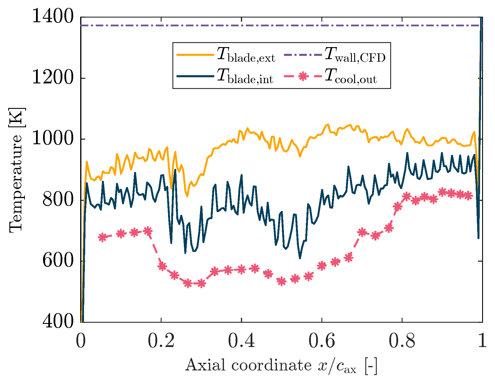
The streamwise temperature profiles are shown as solid lines in Figure 2, while the maximum allowable blade temperature is shown as a dashed line. Despite the use of a total-variation regularisation [27], the numerical differentiation of the total enthalpy profile in Equation (1) introduces some noise in the linear thermal power q ˙ . As a result, the blade external temperature profile shows some oscillations. The oscillations in the blade internal temperature are instead due to two different phenomena: the numerical noise affecting T b , ext and the presence of the cooling channels. The thickness reduction in the vicinity of a cooling channel causes a decrease in the thermal resistance of the blade and thus an increase in temperature. Due to the high heat flux of this application, the temperature variations caused by the thickness reduction are larger than the numerical oscillations. Since they are located close to the cooling channels, the peaks in T b , int (where the thickness is the lowest) are aligned with the points of the T cool , out profile, which mark the centres of the channels. Consistently with the thickness distribution of the blade profile, the difference between T b , ext and T b , int is larger in the central region and lower at the extremities. The sharp peaks at the extremities of the blade are due to numerical differentiation but have no impact on the final solution as they affect only the first and last points of the temperature profile. While the prediction of the 1D model is less accurate at the extremities of the blade because the flow in these regions cannot be accurately described as 1D, inaccuracies in these regions can affect the final solution depending on the extension of the blade section where they occur. In the case of the numerical spikes just mentioned, they only occurred at two points and therefore, they have virtually no effect. If the explicit estimation of the heat transfer coefficient by correlations is introduced, the singularity of the heat transfer coefficient at the leading edge ( h ext x 4 / 5 when x 0 ) reduces considerably the thermal resistance in that region and could lead to unrealistically high temperatures [28]. Since these high temperatures would affect a more extended region than the numerical spikes mentioned above, the final accuracy of the 1D prediction would be lower. For this reason, the external heat transfer profile was not explicitly calculated in this run.
For comparison, in Table 2 are gathered the main mass-averaged outputs of the 1D code for the present cases and for a preliminary case with 15 circular channels. The total coolant-to-gas mass flow ratio is in both cases consistent with values found in the literature for convection-cooled blades. The outlet Mach number in the central part of the blade (where the prediction of the 1D model is expected to be accurate) is within the low subsonic region for the 31 channels case. For the 15-channel case, the non-dimensional pressure drop Δ p cool / p cool , in is not accurate since Equation (6) holds only for low subsonic flows, but it gives an idea of the unfeasibility of the 15-channel solution. It is interesting to notice that the decrease in coolant mass flow, and therefore coolant Mach number, is accompanied by an increase in the average coolant outlet temperature: given the same amount of thermal power, for a reduced amount of coolant, the average temperature change must increase.

3.3. Sensitivity Analysis

One of the most attractive opportunities offered by the 1D code is the possibility of performing sensitivity analyses to study the impact of uncertainties or variations of the input parameters on the solution. After having verified that the majority of the relationships (33 out of 42) are non-linear, a global sensitivity analysis is performed for the 31-channel cooling system using a surrogate model generated with a polynomial chaos expansion (PCE). This technique provides a computationally more economical alternative to Monte Carlo simulations while maintaining acceptable accuracy [29]. To show how uncertainties on h ext affect the results of the 1D code, T w is calculated rather than imposed during this analysis. The coefficients K ext and K int simulating a prediction error of the heat transfer correlations are modelled as Gaussian distributions with zero mean, whereas all the other input parameters are modelled as uniform distributions. The variation ranges used are listed in Table 3.
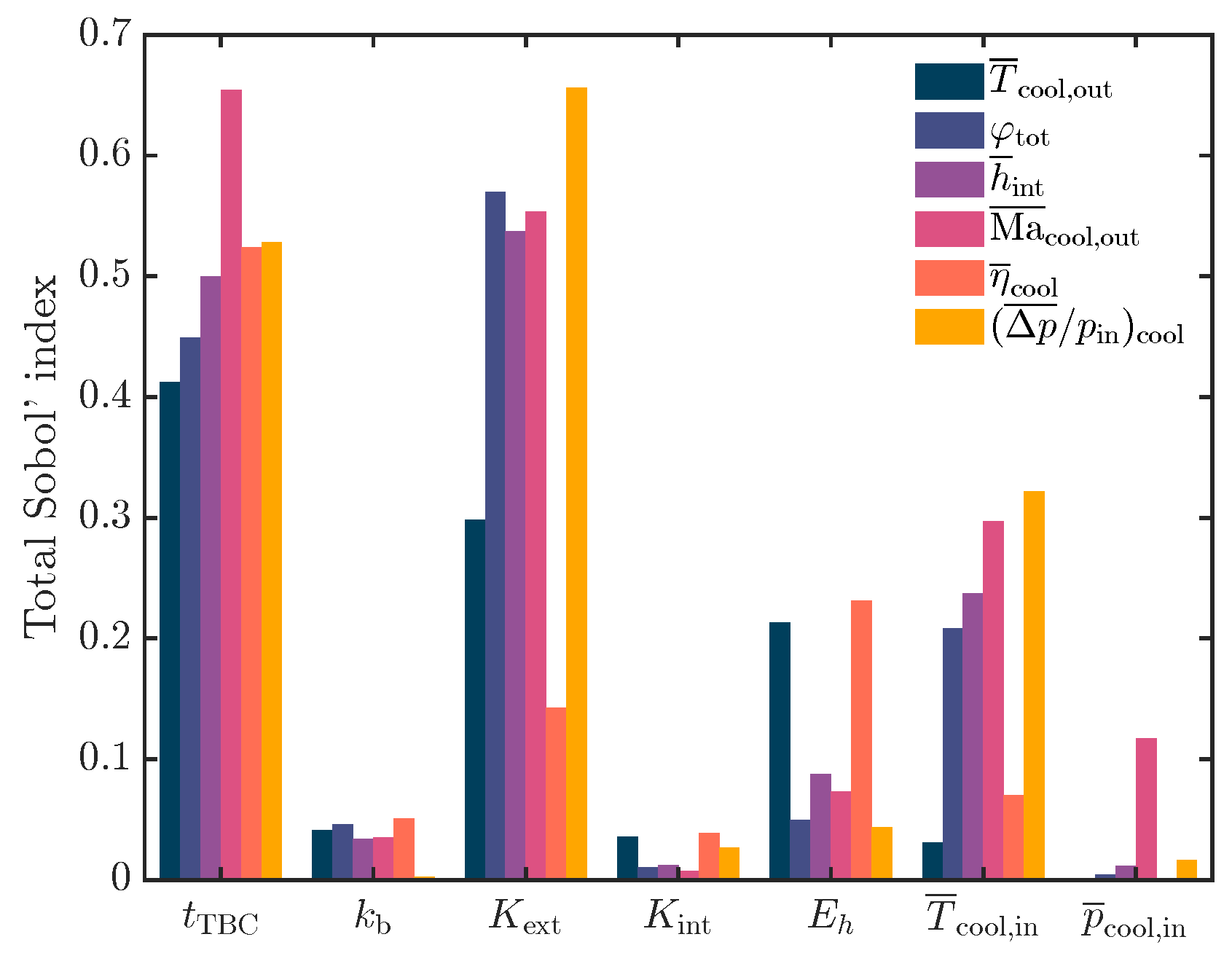
To evaluate quantitatively the impact of the i-th input variable on the j-th output variable, Sobol’ indices are used. In Figure 3 are shown the total Sobol’ indices defined by Equation (7) in [30], where k = 1 , , n and k i .
S tot , i j = 1 Var ( E ( Y j | X k ) ) Var ( Y )
Equation (7) represents the amount of variance of the j-th output variable Y j due to either a variation of the i-th input variable X i or to an interaction between X i and other input variables (so-called “higher order interaction”).
Both the surrogate model and the quantitative sensitivity analysis are performed using UQLab, a MATLAB-based open-source uncertainty quantification framework [31]. MATLAB R2024a is used for both analysis and postprocessing. The PCE used is of 6th order with 1716 basis functions and an oversampling ratio of 3, as suggested by [32]. The order of the expansion has been determined after a convergence analysis.
The coolant Mach number and pressure drop are very sensitive to input variations, supporting the decision to use them as indicators of the feasibility of the solution found by the 1D code (Figure 3). The impact of the blade conductivity is of minor importance, thus justifying the use of a constant mean conductivity in the analysis performed here. The high impact of the TBC is consistent with [17], who highlighted the importance of TBC for reducing the blade temperatures.
Figure 3 also emphasises the non-negligible influence that heat transfer correlations have on the solution of the problem: being notoriously inaccurate ( ± 25 % uncertainty on h ext and ± 10 % on h int ), the solution of the problem is bound to be partially inaccurate. For this reason, the optimised configuration obtained with the 1D mode must be checked against either experimental data or CHT simulations. Moreover, the high sensitivity of the model to variations in h ext rather than in h int justifies the decision in Section 3.2 to avoid the explicit estimation of h ext .
In Figure 3, η cool is the cooling efficiency Equation (8) as defined by [14].
η cool , j = T cool , out , j T cool , in , j T w , j T cool , in , j
In Equation (8), T w , j is averaged using the same area averaged used in Equation (5). The cooling efficiency is bounded between 0 and 1, where 0 corresponds to an infinite mass flow of coolant that acts as a constant temperature heat sink, and 1 corresponds to the coolant undergoing the maximum temperature rise.
The heat enhancement factor E h is defined by Equation (9), where h is the actual heat transfer coefficient and h ref is a reference coefficient, usually that of a smooth wall or that of the system without turbulators (but with non-zero roughness).
E h = h h ref
Equation (9) is a simplified way of evaluating the increase in heat transfer due to a modified geometry that enhances the turbulence of the flow. Its considerable impact on the coolant outlet wall temperature suggests that it may be possible to improve the thermal performance of the system by using turbulators within the cooling channels, such as internal pins or grooves. However, turbulators increase the coolant pressure drop and there is a trade-off between increased heat transfer and pressure loss [17]. With the current geometry, the pressure drop is not negligible; therefore, turbulators are not considered in this analysis.

4. CHT Analysis

4.1. Validation

The CHT solver is validated on the NASA C3X vane experimentally studied by [33]. Similarly to [34], the setup considered is Hylton’s run 112 (transonic case). The computational domain is composed of one solid domain, the blade, and two fluid domains: the external hot gas and the internal cooling channels. The hot gas domain is meshed in Ansys TurboGrid [35] using 2.1 million cells, while the solid blade and the coolant domains are meshed in Ansys Fluent [26] using 2.2 million elements overall. A boundary layer refinement is added to guarantee y + < 1 at the blade wall, thus ensuring that the external boundary layer is properly solved. A grid convergence analysis has been performed and the grid convergence indices (GCIs) calculated on the volume-averaged blade temperature and on the thermal power absorbed by the coolant are 0.28% and 0.72%, respectively. The turbulence model adopted is the k- ω SST model and the simulation is a steady Reynolds-averaged Navier–Stokes (RANS). The vane material is the stainless steel AISI 310 and its properties, extracted from [34], are listed in Table 4.
For this validation case only, both the hot gas and the coolant are modelled as air, considering it as an ideal gas whose properties are listed in Table 5. The values of the parameters used in Sutherland’s law are μ 0 = 1.789 × 10 5 Pa·s, T 0 = 288 K and S = 110 K. This modelling choice is made for consistency with Kumar’s simulations of the NASA C3X vane.
The boundary conditions at the inlets and outlets of the fluid domains, as assigned by [34] and mimicking Hylton’s experimental setup, are listed in Table 6 and Table 7.
The gas inlet Reynolds number is 5.3 × 10⁵. Each cooling channel is assigned the same turbulent intensity I turb = 5 %, the same viscosity ratio μ turb / μ = 10 and the same outlet static pressure p cool , out = 101,325 Pa. The endwalls of both gas and blade domains are adiabatic. Coupled walls are used to model the interface between the fluid domains and the solid domain, thus ensuring a proper solution to the conjugate heat transfer problem.
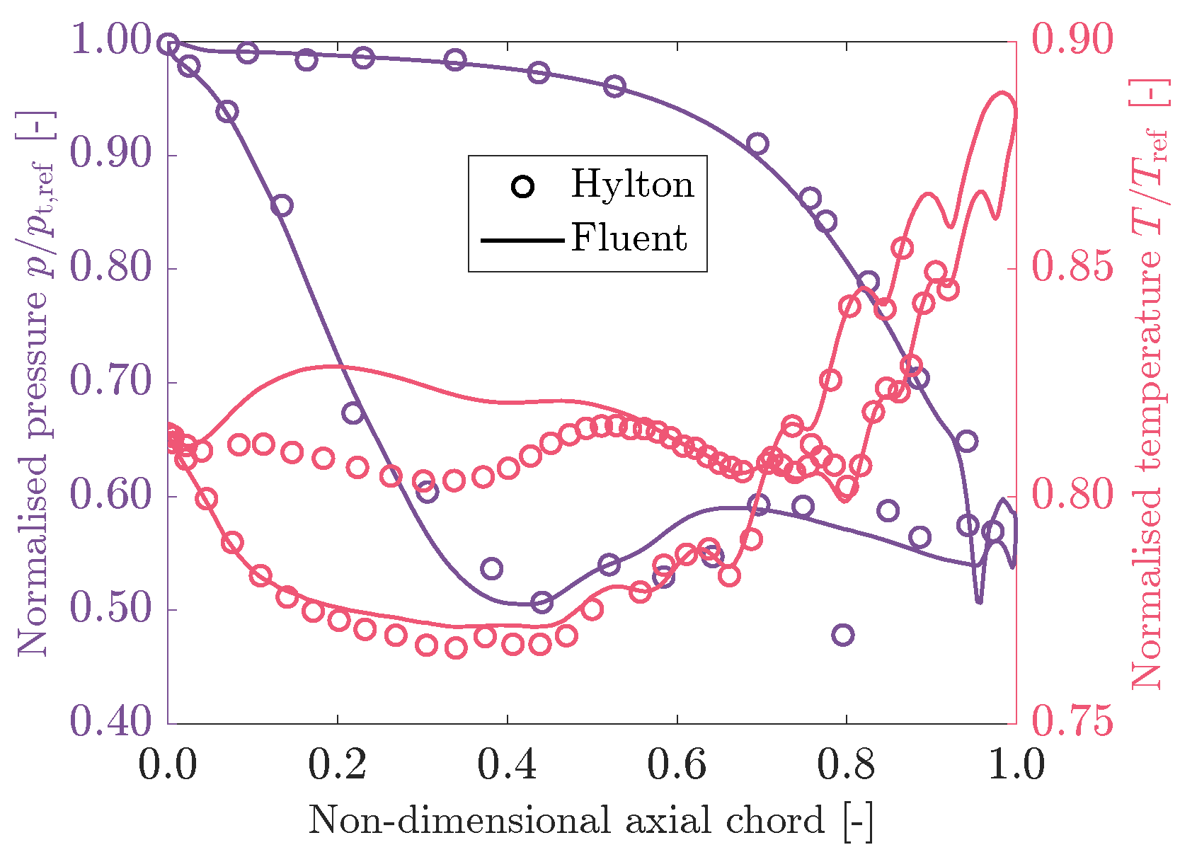
The normalised static pressure p / p t , ref and static temperature T / T ref at the wall extracted from the Fluent case are compared to Hylton’s experimental data in Figure 4.
As in [34], the agreement on the normalised pressure is excellent on both pressure side and suction side, with the exception of a few points in the rear portion of the suction side. The decrease in accuracy on the pressure side when considering the normalised temperature is a known problem in the literature [34,36]. Both studies underlined the importance of the laminar-to-turbulent transition in predicting the wall temperature and the external heat transfer coefficient. Ref. [34], in particular, showed that more sophisticated models, such as the γ - θ transition SST, can improve the accuracy of the prediction but still suffer from locally high errors. As the k- ω SST is widely used and performs well in a wide variety of applications, it is preferred to other models more geared towards specific applications.
Despite these known problems, the agreement between CHT and experimental data is satisfactory and the CHT solver is thus considered as validated.

4.2. Case Setup

A full CHT simulation is performed since no experimental data are available for this RDE technology. The mesh for the hot gas domain is generated in Ansys TurboGrid using 4.7 million cells and ensuring a y + < 1 so that the boundary layer can be properly solved. The solid blade and the coolant domains are meshed in Ansys Fluent using 4.3 million elements overall. The turbulence model adopted is the k- ω SST model. The solids are modelled using constant properties, whereas the fluids use temperature-dependent properties. In particular, the specific heats are modelled using NASA polynomials, whereas both dynamic viscosity and thermal conductivity are modelled using Sutherland’s law. Solid properties are listed in Table 8, whereas fluid properties can be found in [37].
Total pressure, total temperature, and static pressure are assigned at the inlet of the gas domain and are representative of RDE applications, whereas no conditions are assigned at the outlet since the flow is supersonic, as listed in Table 9.
A coupled wall, together with a thin wall resistance, is used to model the gas–TBC–blade interface. The thickness of the TBC is 300 μm. The endwalls of both gas and blade domains are adiabatic. A coupled wall is used to model the interface between cooling channels and the coolant domain. Mass flow rate and total temperature are assigned at the inlet of the cooling channels, whereas static pressure is assigned at the outlets. Both the mass flow rates and the static pressures are extracted from the results of the 1D code run described in Section 3.2 and are listed in Table 1.
For the 15-channel case, a grid convergence analysis has been performed following [38] and using 2 million, 4.9 million, and 9 million cells, monitoring both the blade external temperature and the thermal power absorbed by the coolant. The grid convergence index (GCI) for the 9 million cells grid is below 1.5% when considering the absorbed thermal power and below 0.5% when considering the blade external temperature. Since the overall dimension of the computational domain is unchanged in the 31-channel case, a grid with approximately the same number of elements as the 15-channel fine grid is used for the 31-channel case.

4.3. Results

In this section, only the results of the 31-channel case are analysed, as it was shown in Section 3.2 that the 15-channel solution has a lower performance. The hot gas Mach field and the shock structures are visible in Figure 5.
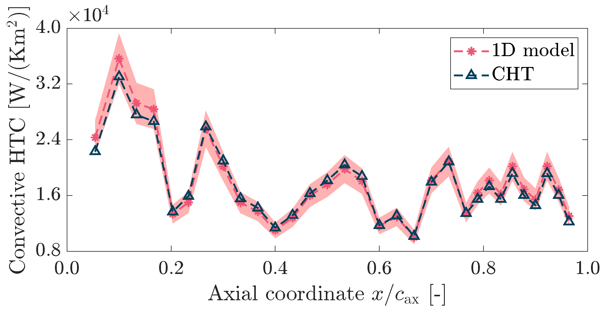
In Figure 6 is shown the wall-function-based internal convective coefficient defined in Equation (10), where T wf is the temperature in the wall-adjacent cell as predicted by the thermal wall function.
h = q ˙ T w T wf
The choice of the wall-function-based coefficient is due to the necessity of keeping the height of the first cell above the sand-grained roughness of the channel’s internal surface. With the chosen average roughness, the non-dimensional wall distance of the first cell would be well above 5; therefore, calculating the heat transfer coefficient using the temperature of the first cell instead of T wf would lead to an incorrect estimation of the convective coefficient. Since the coolant flow at the wall is modelled rather than solved, choosing the wall-function-based coefficient is the most consistent choice. The agreement between 1D code and CHT simulation is excellent: the values extracted from the CHT simulation lie entirely within the ± 10 % uncertainty band of the correlation, with the average error being 2.85 % . The area-averaged external heat transfer coefficient is 2630 W/(K m2), whereas the internal heat transfer coefficients mass-averaged over channels 8–19 is 15,570 W/(K m2).
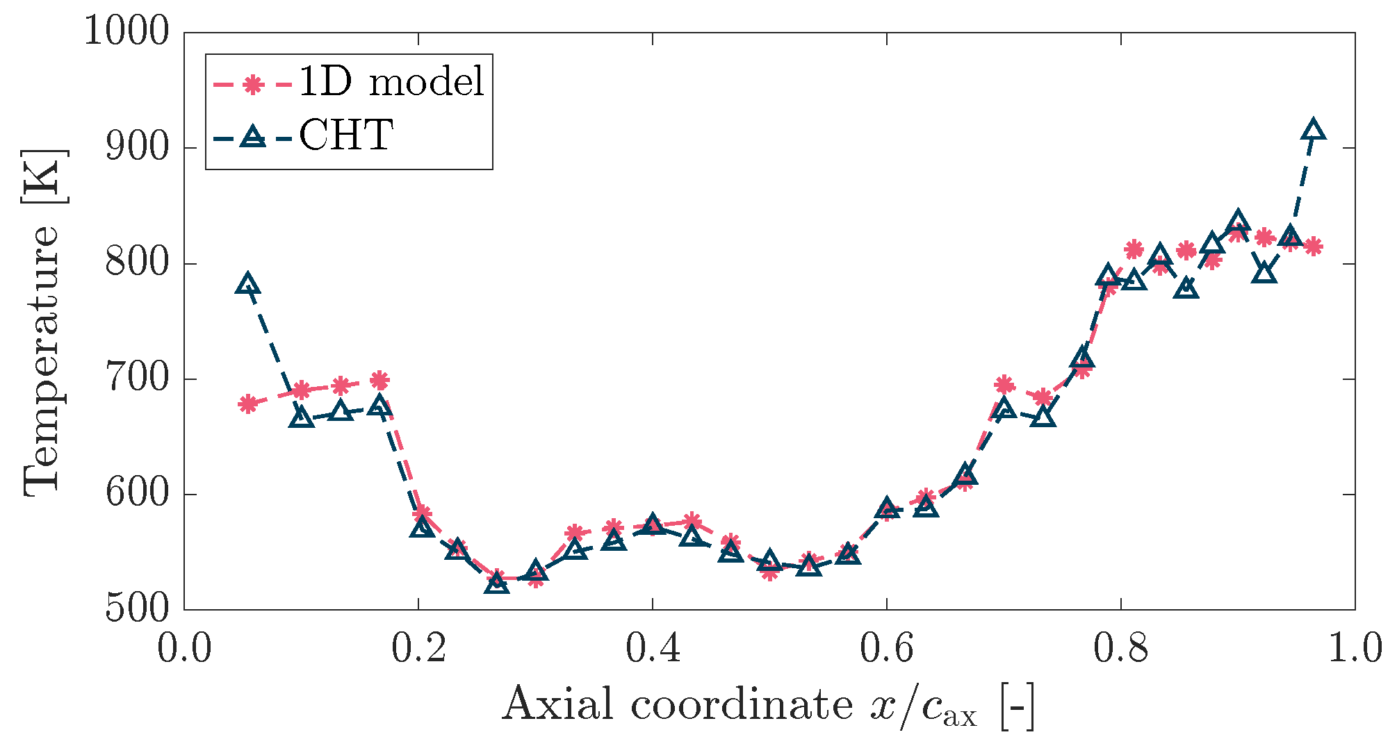
In Figure 7, the coolant outlet temperature predicted by the 1D code is compared to the total temperature at the outlet of the cooling channels as extracted from the CHT simulation. Since the 1D code does not distinguish between total and static temperature, total temperature is used because it is more intimately connected to an absorption of heat. Again, the agreement is excellent: the average error is 1.40 % .
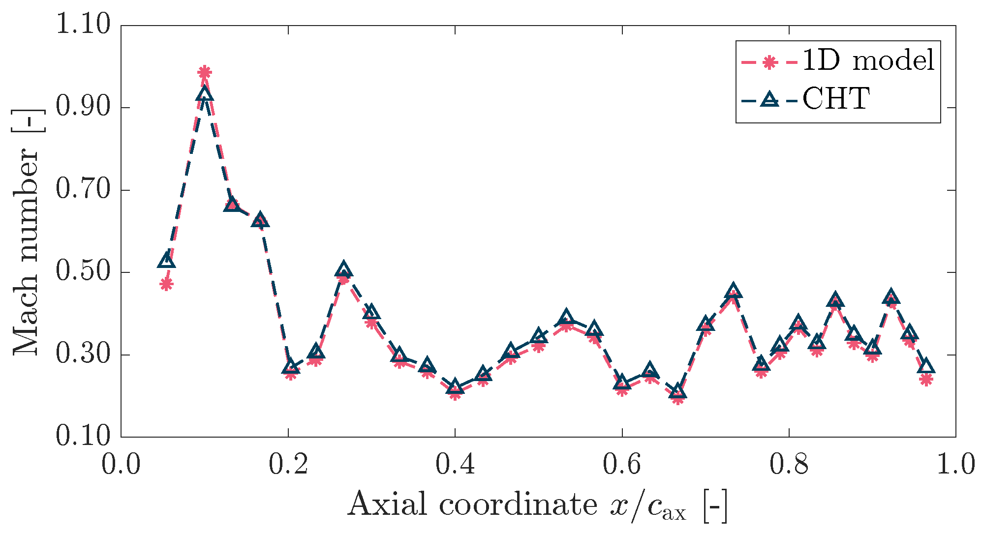
In Figure 8 is shown the coolant Mach number at the outlet of the cooling channels. The outlet coolant Mach number depends on the coolant outlet pressure and, as mentioned in Section 2, the pressure drop Equation (6) can be inaccurate if the Mach is above 0.5. For this reason, the average error is higher and reaches 5.14 % , which is still considered to be satisfactorily small.
The striped wall temperature shown in Figure 9 is due to the presence of the cooling channels, which reduce the temperature locally. It is worth noting that the temperature in Figure 9 is not constant in the spanwise direction, contrary to what was assumed during the development of the 1D model. However, considering that the variation is minor and occurs mostly on the suction side, it is therefore reasonable for the 1D code to assume no radial evolution of the temperature.
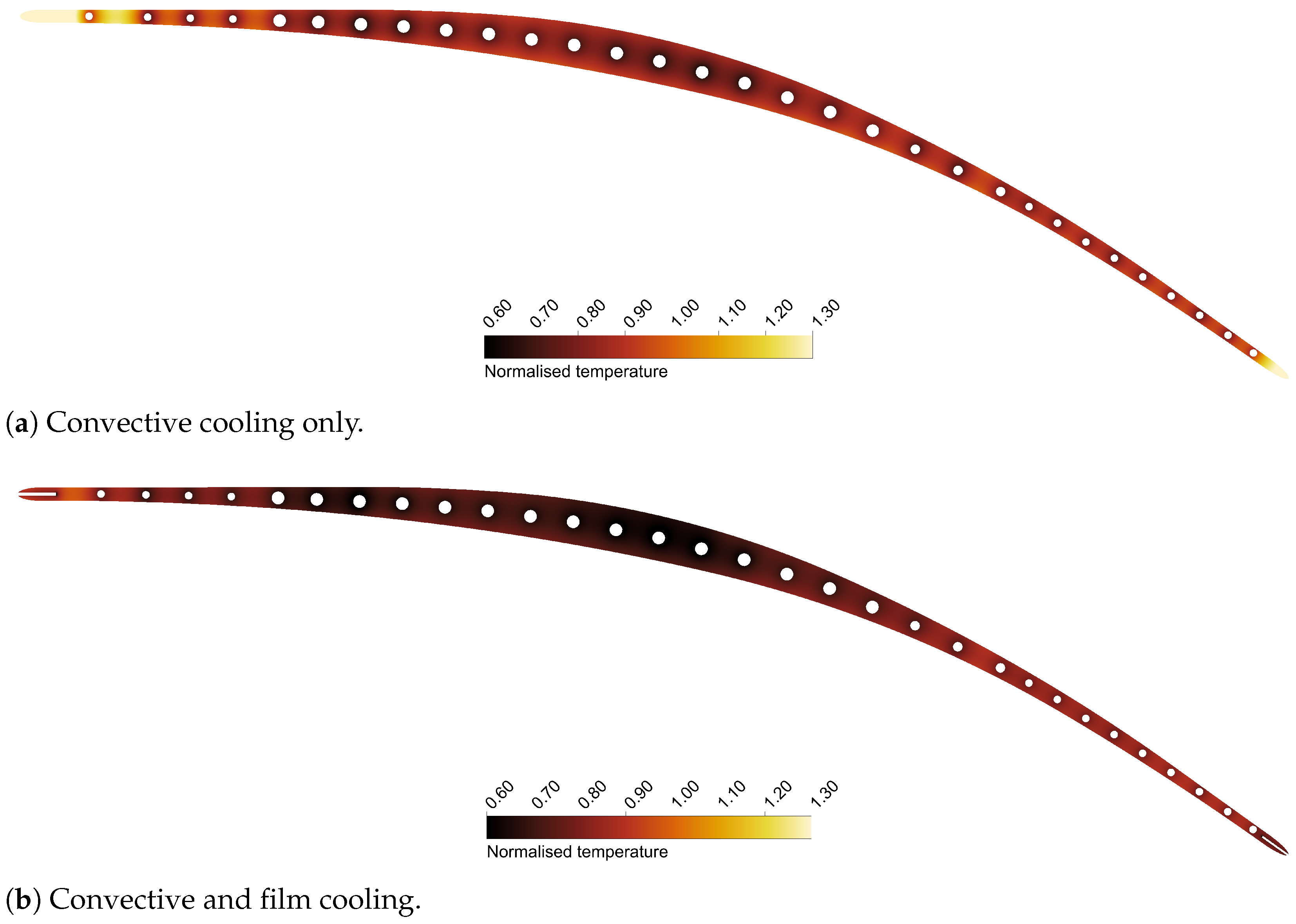
At the extremities of the blade, the thickness is too small to allow for the presence of a cooling channel, which leads to higher temperatures visible in Figure 10a. This suggests that other more effective cooling methods are required in these regions, such as film cooling or impingement cooling. As can be seen in Figure 10a, there are regions where the normalised temperature T / T max , with T max being the Inconel maximum sustainable temperature for prolonged operation (1000 °C, whereas the maximum TBC temperature is set to 1300 °C [39,40]), is close to or above 1. This condition prevents the prolonged operation of the turbine, which is usually around 100,000 h or 15–20 years of discontinuous operation for heavy-duty cycles [39].
As mentioned previously, it may be possible to increase the thermal performance of the system and bring the blade temperature to an acceptable value by introducing turbulators inside the cooling channels, thus increasing the internal heat transfer coefficient while maintaining a convective cooling system. A possible solution may be the use of helical grooves with a helix angle of 45°, which offers the best trade-off between increased heat transfer coefficient and increased pressure drop (and consequent pumping power), as shown by [41]. In this scenario, the 1D model could be effectively used to study several turbulator configurations.
The 1D code can therefore be used successfully during the preliminary design of a cooling system to verify which cooling system design operates in the low subsonic region so that only those are analysed more in-depth with a full CHT simulation.

5. Film Cooling

The internal cooling system successfully reduced the central blade temperatures to within the material’s safe operating limits. However, the leading and trailing edges remain critically hot, as internal cooling alone is insufficient, even with cooling holes placed near the extremities. To address these localised hotspots, an alternative strategy is required. A viable solution to overcome this issue is to inject cooling flow at the leading and trailing edges. The film-cooled blade has two additional channels for the injection of coolant: one at the leading edge, with diameter 0.5 mm and length 6 mm, and one at the trailing edge, with diameter 0.3 mm and length 5 mm. A total of 15 injection cooling channels are considered for both the leading and trailing edges with a uniform distribution in the spanwise direction. Since a finer mesh is required to capture the interaction between the bow shock in front of the blade and the coolant jet, solving the flow around the entire blade would be too computationally expensive. Hence, only the portion of the domain around the injection cooling located at the midspan of the blade is simulated. The meshes are created with Ansys Meshing for the gas domain and Ansys Fluent for the blade and coolant domain, with 1.8 million and 2.3 million elements, respectively. The material properties as well as the hot gas boundary conditions are the same as in Section 4.2. The coolant boundary conditions for the internal channels are obtained from the results of Section 4.2, assuming a linear variation of pressure and temperature in each channel. The injected coolant mass flow rates are 0.50 g/s at the leading edge and 0.05 g/s at the trailing edge, both at a total temperature T t of 709 K and with a turbulent intensity of 5%. The total mass flow rate of coolant injected at the leading and trailing edge is thus 0.388% and 0.033 % of the hot gas mass flow, respectively. The mass flow rates are chosen to minimise the impact on the external hot gas flow field while ensuring a proper cooling action. The total temperature is calculated assuming that air is compressed from ambient conditions to the same total pressure of the hot gas and that the compressor has an isentropic efficiency of 85%.
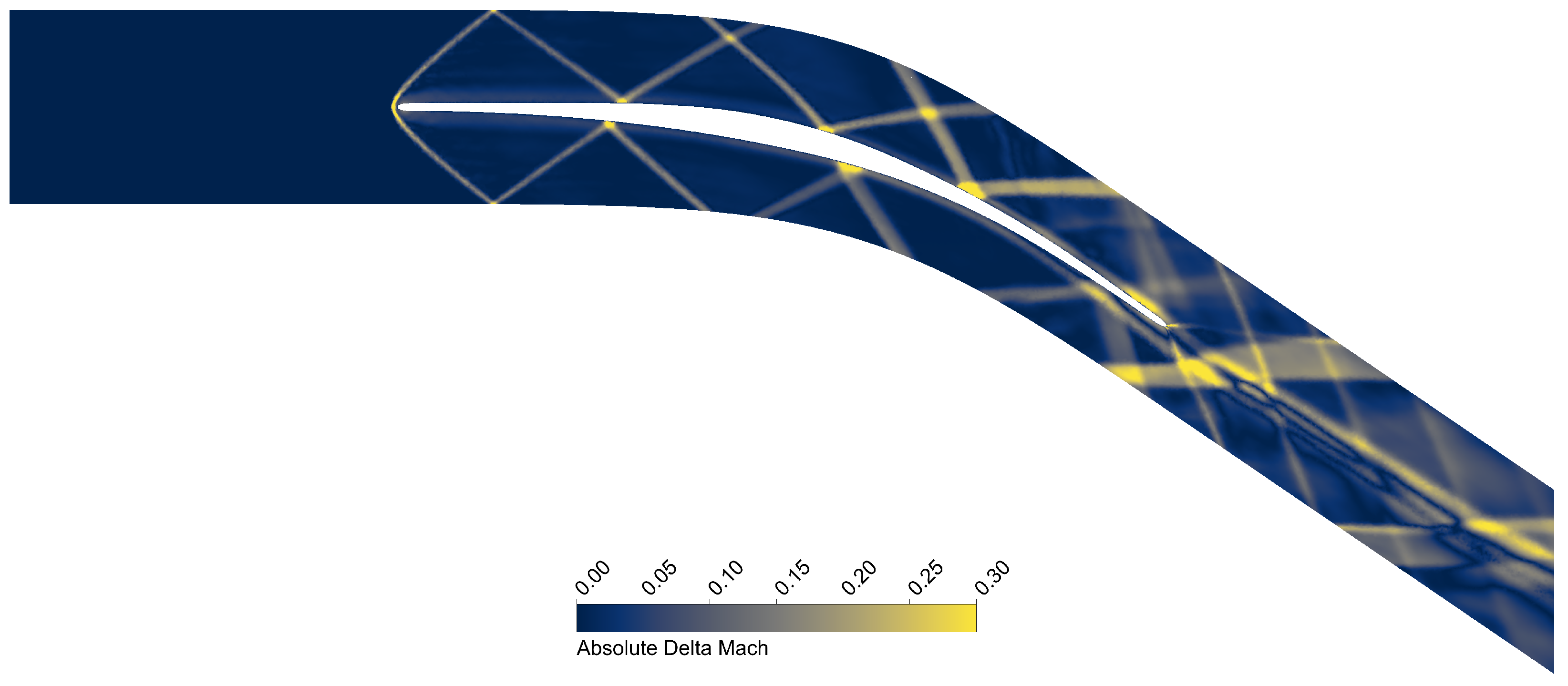
The temperature reductions at the leading and trailing edge are clearly visible in Figure 10b compared to Figure 10a. The absence of hot regions at the leading and trailing edge diminishes the heat conducted towards the central region of the blade, lowering the temperature also there. The disturbance on the external flow field is evaluated in Figure 11 as a difference in Mach number with respect to the case with only convective cooling shown in Figure 5. Since shocks are regions of high gradients, a small change in position creates a great change in Mach number, as visible in Figure 11. Outside of the shocks and their reflections, the Mach number field is almost unperturbed. The interaction between the two opposite fluid streams causes a total pressure loss of 1.82%. Considering that the blade is now able to withstand the high-temperature environment, this loss increase, while not negligible, is acceptable. Overall, coolant injection at the leading and the trailing edge is a possible successful strategy for the thermal control of a RDE blade, as it lowers the temperature of the entire blade without producing excessive disturbances in the external flow field and requiring a modest increase in the amount of coolant mass flow rate. To the authors’ knowledge, this is the first contribution in the literature proposing a solution able to cool down an RDE blade.

6. Feasibility Assessment

6.1. Finite Element Analysis

To assess the structural feasibility of the proposed geometry, a coupled static–thermal analysis is performed in Abaqus 2024 [42]. Inconel 738 properties such as density, Young’s modulus, Poisson’s ratio, thermal conductivity, expansion ratio, and specific heat are modelled as functions of temperature. Data are extracted from [43,44,45]. The pressures of the hot gas and coolant are applied as external load, as well as the heat fluxes at the hot gas–blade and blade–coolant interfaces. The blade is fixed at one endwall and no heat flux is assigned at endwalls, consistently with the CHT setup. Linear coupled temperature-displacement elements are used and, similarly to Section 4, a grid sensitivity analysis is performed. Three grids with an element size of 1 mm, 0.75 mm, and 0.5 mm are used and the GCI on the maximum displacement (local quantity) is 1.66%, whereas the GCI on the total strain energy (integral quantity) is 3.79%. While higher than the GCI obtained for the CHT case, it is still considered satisfactory, as the main objective of this study is the thermal behaviour of the cooling system. The minimum safety factor is 4 in a small region near the hub of the trailing edge and is probably affected by the fixed boundary condition, whereas for the rest of the blade, the safety factor exceeds 8 and is thus compliant with the strictest design methodologies for turbine static components.

6.2. Cooling Power Requirements

To comprehensively assess the cooling requirements, a preliminary evaluation of the associated compression costs is presented. The current cooling strategy necessitates two distinct pressure levels for coolant delivery: approximately 15 bar for film cooling and 35 bar for internal cooling passages. While this evaluation focuses primarily on the stator cooling system, the methodology can be easily extended to include the rotor cascade. Two cooling supply configurations are analysed:
  • Option A, tailored for land-based turbine applications, involves the use of external compressors dedicated to supplying the coolant flow to the stator.
  • Option B, suitable for both aeroengines and land-based applications, leverages the existing Joule–Brayton cycle compressor. To accommodate the elevated pressures required by the internal cooling flow, additional compression stages are introduced. These stages compensate for the pressure gain occurring in the rotating detonation combustor and ensure the coolant reaches the necessary high-pressure level required for internal cooling.
In option A, a double-stage centrifugal compressor is employed to achieve the film cooling pressure level of 15 bar. This is followed by an additional compressor stage to increase the pressure to the 35 bar level required for internal cooling. A cooler is installed between the second and third compressor stages, introducing a pressure loss of approximately 0.5 bar. The key parameters and performance characteristics of all three compressors are summarised in Table 10.
This represents approximately 20% of the power output of the first stage. However, it should be noted that a portion of this power can be recovered by re-injecting the coolant flow back into the main gas path. The coolant mass flow for the stator accounts for roughly 10.5% of the total stage flow, with a corresponding power consumption of approximately 5.2 MW. Assuming comparable cooling requirements for the rotor blades, the total power needed to compress the coolant flow is estimated at around 10 MW.
In option B, a single-stage centrifugal compressor is used to reach the film cooling pressure level, complemented by an additional compressor for the internal cooling pressure requirement. The characteristics of these compressors are detailed in Table 11. For this configuration, a 10% pressure gain across the combustion process is assumed, and the axial compressor efficiency is estimated at 85%. The second compressor stage, responsible for increasing pressure to the internal cooling level, is consistent with that of option A.
While numerous alternative configurations for the compression system exist, the present analysis is intended to support the primary objective of this study: a feasibility assessment of the cooling technology for a supersonic inlet axial turbine stage operating under the extremely demanding conditions of a rotating detonation engine.

7. Conclusions

A 1D model able to predict the thermal field inside a turbine blade and the amount of coolant required is developed. The model is based solely on physical basic principles and is computationally efficient, which allows to run both a qualitative and quantitative sensitivity analysis. The former confirms the non-linear nature of the thermal problem and the latter shows that the coolant outlet Mach number is greatly influenced by variations in the input parameters. Thanks to this sensibility, it is a parameter that should be monitored during an initial exploratory design. The 1D code is used to design and improve an internal cooling system for an RDE turbine, which is then studied through a full CHT analysis. No previous attempts to design an internal cooling system for this new type of machine are available in the literature; hence, the 1D code represents a valuable tool with the potential to fill a gap in both literature and design methodologies. The values predicted by the 1D code for the selected blade and cooling system geometry are in excellent agreement with data available in the literature and with the CHT simulations, thus confirming the accuracy of the tool.
For the supersonic inlet turbine, internal cooling successfully reduces the central blade temperatures below the maximum threshold required for prolonged operation. Additionally, injecting cooling air around the leading and trailing edges forms a protective film to manage hotspot regions effectively. This work demonstrates that with a well-designed internal cooling system and precise cooling strategies for the blade’s critical areas, it is possible to keep the thin, aerodynamically efficient blades of a supersonic turbine within the material’s safe operating temperature limits. To the authors’ knowledge, this is the first study in the literature that suggest a solution able to cool a RDE blade.
The true value of the 1D code here developed lies in the possibility of exploring a vast design space during the preliminary design of a cooling system. Several cooling geometries and configurations can be tested extensively as well as different cooling fluids, cooling inlet conditions, and material properties. This is particularly interesting when input data are uncertain and allows one to perform extensive sensitivity analysis to study the influence of input parameters on the final solution. Moreover, the code can be easily extended to include experimentally tuned correlations or other cooling methods. Few geometric parameters are required to define the cooling system, allowing the designer to rapidly test more configurations focusing only on the main quantities. This is strikingly different from a full CHT analysis, which requires considerable time to set up and run.

Author Contributions

Conceptualization, A.P., N.M. and P.G.; methodology, A.P., N.M. and P.G.; software, A.P.; validation, A.P. and N.M.; formal analysis, A.P. and N.M.; writing—original draft preparation, A.P., N.M. and P.G.; writing—review and editing, A.P., N.M. and P.G.; visualization, A.P.; supervision, N.M. and P.G.; project administration, P.G.; funding acquisition, P.G. All authors have read and agreed to the published version of the manuscript.

Funding

This work was conducted as part of the PRIN 2022 project EnaTech-RDE (Id: 2022BW9SHS), funded by the Italian Ministry of University and Research (MUR).

Data Availability Statement

Data is contained within the article.

Acknowledgments

The authors wish to express their gratitude to Antonio Andreini for providing the CAD models employed for Hylton’s validation case.

Conflicts of Interest

The authors declare no conflicts of interest.

Nomenclature

A g , out blade channel outlet cross sectional aream2
A lat cooling channel lateral aream2
bblade heightm
c ax axial chordm
c p specific heat at constant pressureJ/(kg K)
D h hydraulic diameterm
E h turbulence heat transfer enhancement factor
fDarcy friction factor
hconvective heat transfer coefficient W/(K m2)
h ˜ specific enthalpyJ/kg
Kerror coefficient
kthermal conductivityW/(m K)
MaMach number
m ˙ mass flow ratekg/s
PrPrandtl number
pabsolute pressurePa
q ˙ thermal powerW
q ˙ linear thermal powerW/m
q ˙ heat fluxW/m2
R specific gas constantJ/(kg K)
R a average surface roughnessμm
SSobol’ index
StStanton number
tthicknessm
Tabsolute temperatureK
xaxial coordinatem
y + non-dimensional wall distance

Greek Symbols

α b blade metal angle
η cooling efficiency
φ coolant-to-gas mass flow ratio
μ dynamic viscosity
ρ density

Subscripts

bblade
ccooling channel
coolcoolant
extexternal (hot gas side)
ggas
intinternal (coolant side)
recrecovery
ttotal quantity
wwall

Superscripts

( ) ¯ average value

Acronyms

CFDcomputational fluid dynamics
CHTconjugate heat transfer
GCIgrid convergence index
PCEpolynomial chaos expansion
RANSReynolds-averaged Navier–Stokes
RDErotating detonation engine
TBCthermal barrier coating

Appendix A. Pressure Drop Estimation

The four terms in Equation (6) accounting for blade and cooling system geometry, cooling fluid, coolant conditions, and blade thermal field are detailed in Equation (A1). With respect to [15], the Chilton–Colburn analogy St = ( f / 8 ) Pr 2 / 3 is used in place of the Reynolds analogy St = f / 8 , St being the Stanton number. Furthermore, since the internal cooling arrangement studied in this work allows one to use coolants different from air and to change freely the coolant boundary conditions, the simplification ( R cool / R g ) ( p g , out / p cool , in ) 1 is not made.
K geo = A g , out A ch 2 b D h f 2
K cool , type = R cool R g
K cool , cond = p g , out p cool , in T ¯ cool T g , out
K th , b = T b , int T ¯ cool 1 Pr cool 2 / 3 + 2
Equation (6) is derived under the assumption that the Mach number is small enough that p t p and T t T , which strictly holds if Ma < 0.1 [15]. However, due to other assumptions whose validity limits are not clearly studied in [15], it is difficult to precisely set a validity limit for the pressure drop formula. For this reason, it is safe to assume that this is always a preliminary estimate whenever Ma > 0.1 .

References

  1. Heiser, W.H.; Pratt, D.T. Thermodynamic cycle analysis of pulse detonation engines. J. Propuls. Power 2002, 18, 68–76. [Google Scholar] [CrossRef]
  2. Paxson, D.E.; Naples, A. Numerical and analytical assessment of a coupled rotating detonation engine and turbine experiment. In Proceedings of the AIAA SciTech Forum—55th AIAA Aerospace Sciences Meeting, Grapevine, TX, USA, 9–13 January 2017; pp. 1–13. [Google Scholar] [CrossRef]
  3. Sousa, J.; Paniagua, G.; Collado-Morata, E. Analysis of the aerodynamic losses in a supersonic turbine. Am. Soc. Mech. Eng. Power Div. (Publication) POWER 2017, 1, 1–7. [Google Scholar] [CrossRef]
  4. Anand, V.; Gutmark, E. Rotating detonation combustors and their similarities to rocket instabilities. Prog. Energy Combust. Sci. 2019, 73, 182–234. [Google Scholar] [CrossRef]
  5. Schwer, D.; Kailasanath, K. Numerical Investigation of Rotating Detonation Engines. In Proceedings of the 46th AIAA/ASME/SAE/ASEE Joint Propulsion Conference and Exhibit, Nashville, TN, USA, 25–28 July 2010; Volume 33, pp. 2195–2202. [Google Scholar] [CrossRef]
  6. Paniagua, G.; Iorio, M.C.; Vinha, N.; Sousa, J. Design and analysis of pioneering high supersonic axial turbines. Int. J. Mech. Sci. 2014, 89, 65–77. [Google Scholar] [CrossRef]
  7. Sousa, J.; Paniagua, G. Entropy Minimization Design Approach of Supersonic Internal Passages. Entropy 2015, 17, 5593–5610. [Google Scholar] [CrossRef]
  8. Mushtaq, N.; Colella, G.; Gaetani, P. Design and Parametric Analysis of a Supersonic Turbine for Rotating Detonation Engine Applications. Int. J. Turbomach. Propuls. Power 2022, 7, 1. [Google Scholar] [CrossRef]
  9. Mushtaq, N.; Persico, G.; Gaetani, P. The role of endwall shape optimization in the design of supersonic turbines for rotating detonation engines. In Proceedings of the ASME Turbo Expo. American Society of Mechanical Engineers, Rotterdam, The Netherlands, 13–17 June 2022; Volume 10-B. [Google Scholar] [CrossRef]
  10. Grasa, S.; Paniagua, G. Design and Characterization of Highly Diffusive Turbine Vanes Suitable for Transonic Rotating Detonation Combustors. Int. J. Turbomach. Propuls. Power 2024, 9, 18. [Google Scholar] [CrossRef]
  11. Lozano, F.; Paniagua, G. Airfoil leading edge blowing to control bow shock waves. Sci. Rep. 2020, 10, 21922. [Google Scholar] [CrossRef] [PubMed]
  12. Nambiar, S.; Ananno, A.A.; Titus, H.; Wiberg, A.; Tarkian, M. Multidisciplinary Automation in Design of Turbine Vane Cooling Channels. Int. J. Turbomach. Propuls. Power 2024, 9, 7. [Google Scholar] [CrossRef]
  13. Filinov, E.; Kuz’michev, V.; Yu Tkachenko, A.; Ostapyuk, Y.; Krupenich, I. Estimation of cooling flow rate for conceptual design stage of a gas turbine engine. Proc. Inst. Mech. Eng. Part A J. Power Energy 2021, 235, 2014–2021. [Google Scholar] [CrossRef]
  14. Jordal, K. Gas Turbine Cooling Modeling–Thermodynamic Analysis and Cycle Simulations. Master’s Thesis, Lund Institute of Technology, Lund, Sweden, 1999. [Google Scholar]
  15. Ainley, D.G. Internal Air-Cooling for Turbine Blades. A General Design Survey; Technical Report; Aeronautical Research Council: London, UK, 1957. [Google Scholar]
  16. Horlock, J.H.; Torbidoni, L. Turbine Blade Cooling: The Blade Temperature Distribution. Proc. Inst. Mech. Eng. Part A J. Power Energy 2006, 220, 343–353. [Google Scholar] [CrossRef]
  17. Consonni, S. Performance Prediction of Gas/Steam Cycles for Power Generation. Ph.D. Thesis, Princeton University, Princeton, NJ, USA, 1992. [Google Scholar]
  18. Sciubba, E. Air-cooled gas turbine cycles—Part 1: An analytical method for the preliminary assessment of blade cooling flow rates. Energy 2015, 83, 104–114. [Google Scholar] [CrossRef]
  19. Masci, R.; Sciubba, E. A Lumped Thermodynamic Model of Gas Turbine Blade Cooling: Prediction of First-Stage Blades Temperature and Cooling Flow Rates. J. Energy Resour. Technol. 2018, 140, 020901. [Google Scholar] [CrossRef]
  20. Torbidoni, L.; Horlock, J.H. A New Method to Calculate the Coolant Requirements of a High-Temperature Gas Turbine Blade. J. Turbomach. 2005, 127, 191–199. [Google Scholar] [CrossRef]
  21. Jordal, K.; Torbidoni, L.; Massardo, A.F. Convective Blade Cooling Modelling for the Analysis of Innovative Gas Turbine Cycles. In Proceedings of the Volume 2: Coal, Biomass and Alternative Fuels; Combustion and Fuels; Oil and Gas Applications; Cycle Innovations. American Society of Mechanical Engineers, New Orleans, LA, USA, 4–7 June 2001; Volume 2, pp. 1–8. [Google Scholar] [CrossRef]
  22. Torbidoni, L.; Massardo, A.F. Analytical Blade Row Cooling Model for Innovative Gas Turbine Cycle Evaluations Supported by Semi-Empirical Air-Cooled Blade Data. J. Eng. Gas Turbines Power 2004, 126, 498–506. [Google Scholar] [CrossRef]
  23. Incropera, F.P.; DeWitt, D.P.; Bergman, T.L.; Lavine, A.S. Fundamentals of Heat and Mass Transfer, 6th ed.; John Wiley and Sons, Inc.: Hoboken, NJ, USA, 2007. [Google Scholar]
  24. Gnielinski, V. On heat transfer in tubes. Int. J. Heat Mass Transf. 2013, 63, 134–140. [Google Scholar] [CrossRef]
  25. van de Noort, M.; Ireland, P.T. Genetic Algorithm-Based Optimisation of a Double-Wall Effusion Cooling System for a High-Pressure Turbine Nozzle Guide Vane. Int. J. Turbomach. Propuls. Power 2024, 9, 6. [Google Scholar] [CrossRef]
  26. Ansys® Fluent, Release 2023 R2; Ansys: Canonsburg, PA, USA, 2023.
  27. Chartrand, R. Numerical Differentiation of Noisy, Nonsmooth Data. ISRN Appl. Math. 2011, 2011, 1–11. [Google Scholar] [CrossRef]
  28. Pinardi, A.; Mushtaq, N.; Gaetani, P. Development of a reduced order model for turbine blade cooling design. In Proceedings of the 16th European Turbomachinery Conference, Hannover, Germany, 24–28 March 2025. paper n. ETC2025-226. [Google Scholar]
  29. Marelli, S.; Lüthen, N.; Sudret, B. UQLab User Manual—Polynomial Chaos Expansions; Technical Report; Chair of Risk, Safety and Uncertainty Quantification, ETH Zurich: Zurich, Switzerland, 2022. [Google Scholar]
  30. Marelli, S.; Lamas, C.; Konakli, K.; Mylonas, C.; Wiederkehr, P.; Sudret, B. UQLab User Manual—Sensitivity Analysis; Technical Report; Chair of Risk, Safety and Uncertainty Quantification, ETH Zurich: Zurich, Switzerland, 2022. [Google Scholar]
  31. Marelli, S.; Sudret, B. UQLab: A Framework for Uncertainty Quantification in Matlab. In Proceedings of the Vulnerability, Uncertainty, and Risk, Reston, VA, USA, 7 July 2014; pp. 2554–2563. [Google Scholar] [CrossRef]
  32. Hadigol, M.; Doostan, A. Least squares polynomial chaos expansion: A review of sampling strategies. Comput. Methods Appl. Mech. Eng. 2018, 332, 382–407. [Google Scholar] [CrossRef]
  33. Hylton, L.D.; Mihelc, M.S.; Turner, E.R.; Nealy, D.A.; York, R.E. Analytical and Experimental Evaluation of the Heat Transfer Distribution over the Surfaces of Turbine Vanes; Technical Report; NASA: Washington, DC, USA, 1983. [Google Scholar]
  34. Kumar, A.; Pathak, M. Conjugate heat transfer analysis of internally cooled superalloy turbine blades with grooved channels. Phys. Fluids 2023, 35, 095112. [Google Scholar] [CrossRef]
  35. Ansys® TurboGrid; Release 2023 R2; Ansys: Canonsburg, PA, USA, 2023.
  36. Facchini, B.; Magi, A.; Scotti Del Greco, A. Conjugate heat transfer simulation of a radially cooled gas turbine vane. In Proceedings of the ASME Turbo Expo 2004: Power for Land, Sea, and Air, Vienna, Austria, 14–17 June 2004; Volume 3, pp. 951–961. [Google Scholar] [CrossRef]
  37. Pinardi, A. Development of a Reduced Order Model for Turbine Cooling Design. Master’s Thesis, Politecnico di Milano, Milano, Italy, 2024. [Google Scholar]
  38. Celik, I.B.; Ghia, U.; Roache, P.J.; Freitas, C.J.; Coleman, H.; Raad, P.E. Procedure for estimation and reporting of uncertainty due to discretization in CFD applications. J. Fluids Eng. Trans. ASME 2008, 130, 0780011–0780014. [Google Scholar] [CrossRef]
  39. Gülen, S.C. Gas Turbines for Electric Power Generation; Cambridge University Press: Cambridge, UK, 2019. [Google Scholar] [CrossRef]
  40. Lima, R.S. Perspectives on Thermal Gradients in Porous ZrO2-7–8 wt.(YSZ) Thermal Barrier Coatings (TBCs) Manufactured by Air Plasma Spray (APS). Coatings 2020, 10, 812. [Google Scholar] [CrossRef]
  41. Han, J.C.; Park, J.S.; Lei, C.K. Heat Transfer Enhancement in Channels With Turbulence Promoters. J. Eng. Gas Turbines Power 1985, 107, 628–635. [Google Scholar] [CrossRef]
  42. Abaqus, release 2024; Dassault Systèmes: Vélizy-Villacoublay, France, 2024.
  43. INCO. Alloy IN-738 Technical Data—A Practical Guide To the Use of Nickel-Containing Alloys; Technical Report; Nickel Institute: Durham, NC, USA, 2020. [Google Scholar]
  44. Zhang, P.; Song, Y.; Xia, Z. Exact mathematical formulas for wall-heat flux in compressible turbulent channel flows. Acta Mech. Sin. 2022, 38, 321403. [Google Scholar] [CrossRef]
  45. Zaretsky, E.B.; Kanel, G.I.; Razorenov, S.V.; Baumung, K. Impact strength properties of nickel-based refractory superalloys at normal and elevated temperatures. Int. J. Impact Eng. 2005, 31, 41–54. [Google Scholar] [CrossRef]
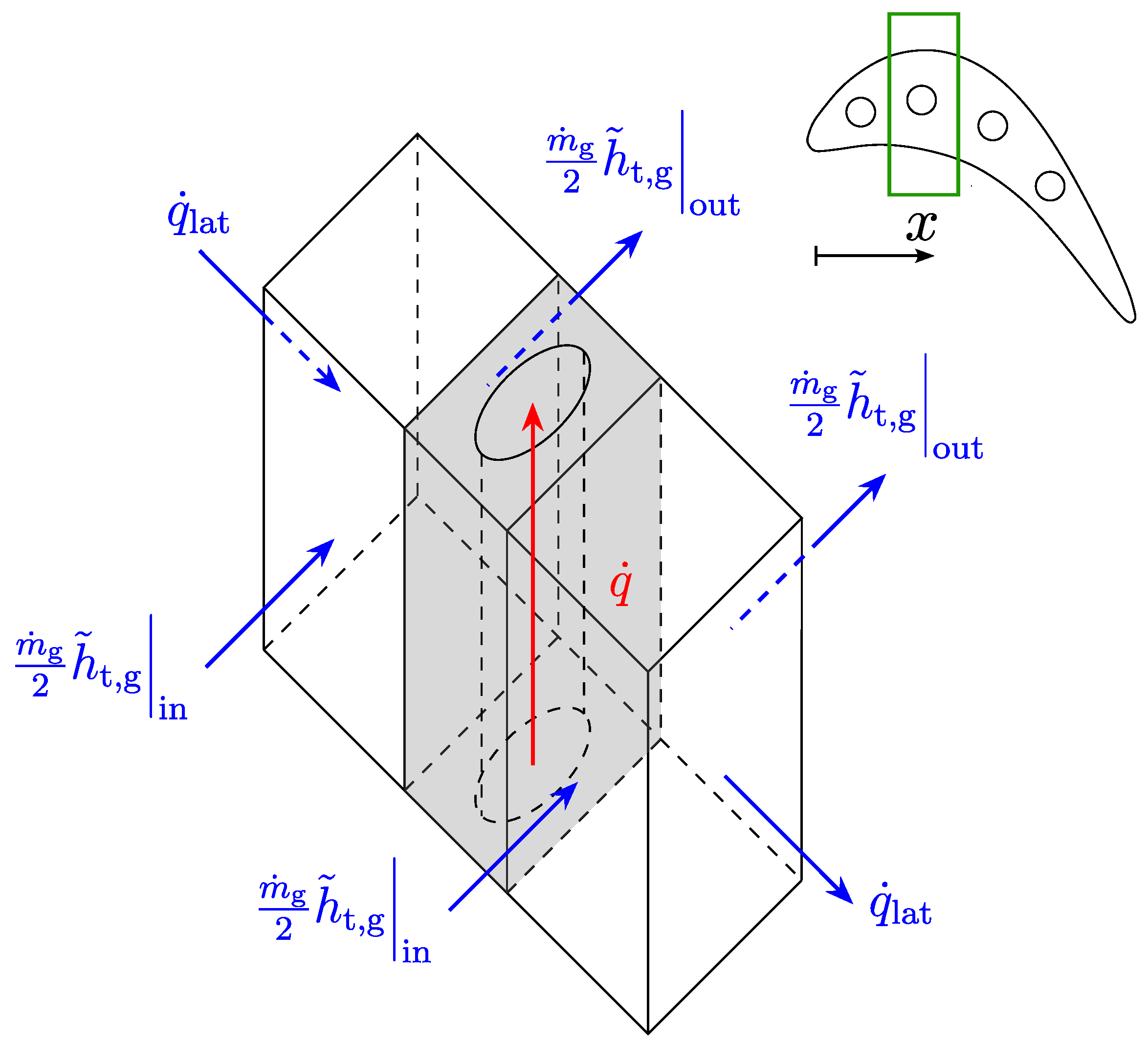
Figure 1. Infinitesimal control volume comprising the metallic blade with a representative cooling channel and both the gas and coolant domains. The blue arrows represent the hot gas thermal powers, whereas the red arrow represents the coolant thermal power. The position of the infinitesimal slice in the bladed row is highlighted in green in the top right corner.
Ijtpp 10 00037 g001
Figure 2. Streamwise temperature distributions predicted by the 1D code. The coolant outlet temperatures are defined only where the channels exist; here, they are joined with a dashed line to appreciate their trend. The wall temperature imposed in the CFD simulation is shown as a dash-dotted line.
Ijtpp 10 00037 g002
Figure 3. Total Sobol’ indices. The impact that a variation in one of the 7 inputs on the horizontal axis has on each of the 6 outputs is measured by the total Sobol’ index of the corresponding colour. With the exceptions of φ tot , all outputs are mass-averaged.
Ijtpp 10 00037 g003
Figure 4. Comparison of normalised pressure p / p t , ref and temperature T / T ref distributions as extracted from Fluent and experimentally measured by [33].
Ijtpp 10 00037 g004
Figure 5. Hot gas Mach field for the 31-channel case.
Ijtpp 10 00037 g005
Figure 6. Comparison between the internal convective heat transfer coefficient as predicted by the 1D code and as extracted from the CHT simulation. The shaded area represents the uncertainty of the Gnielinski correlation.
Ijtpp 10 00037 g006
Figure 7. Comparison between the outlet coolant temperature as predicted by the 1D code and as extracted from the CHT simulation. For consistency with the 1D code, which does not distinguish between total and static coolant temperature, the temperature extracted from the CHT simulation is the total one.
Ijtpp 10 00037 g007
Figure 8. Comparison between the outlet coolant Mach number as predicted by the 1D code and as extracted from the CHT simulation.
Ijtpp 10 00037 g008
Figure 9. TBC superficial temperature extracted from the CHT simulation. The pressure side is on the left and the suction side is on the right. The boundary conditions for the simulation have been extracted from the 1D code.
Ijtpp 10 00037 g009
Figure 10. Normalised temperature field T / T max inside the blade at midspan. Following [40], T max is set to 1000 °C. For the sake of comparison, in the convective cooling case, the contour plot is capped to 1.30, as any value higher than this would be meaningless.
Ijtpp 10 00037 g010
Figure 11. Mach number difference between the case with convective and film cooling and the case with only convective cooling. The difference is limited to 0.30 for ease of visualisation.
Ijtpp 10 00037 g011
Table 1. Coolant boundary conditions for the case under study.
Channel D h m ˙ cool T t , in , cool p out , cool I turb
[mm][g/s][K][bar][%]
11.23.8940027.465
21.25.6340019.245
31.24.6940023.805
41.24.5240024.575
52.07.6040033.095
62.08.6940032.515
72.013.840029.645
82.011.240031.185
92.08.4740032.625
102.07.7740032.955
112.06.3140033.605
122.07.2140033.205
132.08.7840032.475
142.09.7040031.925
152.010.840031.115
162.010.040031.495
172.06.4840033.435
182.07.2440032.985
192.05.7640033.615
201.55.0240030.075
211.55.8140028.325
221.53.8040031.995
231.22.5840030.405
241.22.8840028.915
251.22.5840030.185
261.23.1940027.585
271.22.6840029.735
281.22.4540030.475
291.23.1940027.415
301.22.6940029.535
311.22.0840031.735
Table 2. Main outputs of the 1D code for the cases with 15 and 31 cooling channels. Results have been averaged using a mass average over the central channels (4–10 for the 15-channel case and 8–19 for the 31-channel case).
QuantitySymbolUnitValue
15 ch.31 ch.
Total coolant-to-gas φ tot %11.8510.74
mass flow ratio
Coolant outlet Ma ¯ cool , out 1.040.292
Mach number
Coolant outlet T ¯ cool , out K550562
temperature
Coolant percentage ( Δ p ¯ / p in ) cool %37.07.53
pressure drop
Table 3. Range of parameters investigated in the sensitivity analysis.
QuantityUnitRange Studied
t TBC μm100–400
k b W/(K m)16–28
K ext %−25 to +25
K int %−10 to +10
E h 1–3
T cool , i K400–550
p cool , i bar25–40
Table 4. AISI 310 material properties.
DensitySpecific HeatThermal Conductivity
[kg/m3][J/(kg K)][W/(K m)]
7900585.2 6.13 + 0.0182 T
Table 5. Air properties used for the validation case.
QuantityUnitLaw
Molecular weightkm/kmol28.96
Specific heatJ/(kg K) 944.23 + 0.189 T
Thermal conductivityW/(K m) 0.00932 + 0.000058 T
Dynamic viscosityPa·s μ 0 T T 0 1.5 T 0 + S T + S
Table 6. Hot gas boundary conditions for the validation case.
QuantityUnitValue
Inlet total pressurebar3.22
Inlet total temperatureK783
Outlet static pressurebar1.90
Turbulent intensity%8.30
Turbulent length scalemm0.782
Table 7. Coolant boundary conditions for the validation case.
ChannelDiameterMass Flow RateInlet Total Temperature
[mm][g/s][K]
16.307.79393.3
26.306.58393.1
36.306.34375.2
46.306.66381.0
56.306.52359.2
66.306.72419.1
76.306.33373.0
83.102.26371.6
93.101.38426.9
101.980.68451.4
Table 8. TBC and blade material properties.
MaterialDensitySpecific HeatThermal Conductivity
[kg/m3][J/(kg K)][W/(K m)]
Inconel 738811065022.5
7YSZ60004701.50
Table 9. Hot gas boundary conditions for the case under study.
QuantityUnitValue
Inlet total pressurebar15.0
Inlet total temperatureK2340
Inlet static pressurebar1.94
Turbulent intensity%5
Turbulent viscosity ratio5
Table 10. Key parameters and performance indicators of the three compressors required in option A.
Stage 123
Mass flow ratekg/s9.29.28.8
Inlet pressurebar14.514.5
Inlet temperatureK300502300
PowerMW1.872.370.93
Rotation speedrpm30,00056,70056,700
Outlet pressurebar4.51535
Outlet temperatureK502757400
Max diameterm0.700.450.25
Isentropic efficiency%808181
Table 11. Key parameters and performance indicators of the two compressors required in option B.
Stage 12
Mass flow ratekg/s9.28.8
Inlet pressurebar13.614.5
Inlet temperatureK690300
PowerMW0.210.93
Rotation speedrpm14,80056,700
Outlet pressurebar1535
Outlet temperatureK715400
Max diameterm0.500.25
Isentropic efficiency%8581
Disclaimer/Publisher’s Note: The statements, opinions and data contained in all publications are solely those of the individual author(s) and contributor(s) and not of MDPI and/or the editor(s). MDPI and/or the editor(s) disclaim responsibility for any injury to people or property resulting from any ideas, methods, instructions or products referred to in the content.