Abstract
Stability theory offers a practical method on parametric studies that encompass scales in the boundary layer typically not captured in Large Eddy (LES) or Reynolds-Averaged Navier–Stokes (RANS) simulations. We investigated the transition modes of a Low-Pressure Turbine (LPT) with Linear Stability Theory (LST) and Linear Parabolized Stability Equations (LPSEs) over a wider parametric space. A parametric study was done to examine the wall-shear stress, shape factor, momentum thickness, as well as the growth rate and N-factor envelope. Additionally, the methodology was applied to active control techniques like suction and blowing. The results are consistent with the expected physical behavior and initial observations, while also offering a quantitative description of trends in frequencies, amplitude growth, and wavelengths. This confirms the suitability of the two stability theories, laying the base for their future validation to ensure accuracy and reliability.
1. Introduction
In this study, the transition from laminar to turbulent boundary layer (BL) flow in a Low-Pressure Turbine (LPT) was examined. As aero engines are advanced to minimize environmental impact, modern high-efficiency LPT designs are increasingly focused to operate at transonic flow conditions with an exit Mach number of 0.8 or higher and with high aerodynamic loading. With Reynolds numbers in the range of 100,000 or less at cruise conditions, the various laminar–turbulent boundary layer transition phenomena are crucial in the overall loss production of a given design. The time and length scales involved in boundary layer transition necessitate full Direct Numerical Simulations (DNS), which are generally impractical during the design phase. Conversely, transition correlations such as Abu–Ghannam Shaw (AGS) [1] do not capture design improvement trends effectively.
Effectively controlling transition is essential for maintaining an efficient flow pattern and preventing undesirable occurrences, such as laminar separation bubbles (LSBs). As outlined by Reshotko and White [2], transition can follow different paths, with a distinction between a low disturbance environment, resulting in a natural transition, and a high disturbance environment, leading to a bypass transition. The usage of boundary layer stability theory to study the transition of the flow in the LPT has been rarely attempted and is commonly rejected due to the elevated levels of Free Stream Turbulence Intensity (FSTI). However, the LPT does exhibit multi-modal transition paths and recent DNS have shown an overlap between natural and bypass transition modes. This interaction involves both Tollmien–Schlichting (TS) waves and Klebanoff modes, and is influenced by both the level of FSTI and the boundary layer receptivity. The latter refers to the BL ability to respond to external perturbations and convert them into internal instabilities. Additionally, operating at low Reynolds numbers often leads to the formation of laminar separation bubbles (LSBs), which negatively impact aerodynamic performance [3,4]. Various control methods exist to manage this phenomenon, using both passive and active techniques [5]. Furthermore, the interaction between the wake and the boundary layer plays a crucial role in maintaining boundary layer stability.
Recent investigations into the BL transition in LPT applications have used several methods, including Direct Numerical Simulation (DNS), Large Eddy (LES), and Reynolds-Averaged Navier–Stokes (RANS) simulations, or software such as the Multiple Blades Interacting Streamtube Euler Solver (MISES) [6,7,8,9,10]. However, DNS and LES simulations are highly computationally expensive, while RANS are insufficient for accurately capturing the early stage of the natural transition. Additionally, existing software such as MISES rely on correlations, similar to the AGS transition criterion. Therefore, this study aimed to investigate the early stages of the BL transition in an LPT using stability theories that ensure high accuracy while maintaining a low computational cost. Specifically, the Linear Stability Theory (LST) and Parabolized Stability Equations (PSEs) are employed, implemented in the in-house tool VESTA (von Karman Institute Extensible Stability and Transition Analysis). Specifically, a parametric study under four flow conditions, as shown in Table 1, was conducted. Additionally, an investigation on the effects of typical active flow control techniques, such as suction and blowing, on the BL transition onset location was conducted.

Table 1.
Parametric flow conditions.
For this research, the LPT blade geometry from the EU program SPLEEN, led by the von Karman Institute, was considered, to demonstrate the usefulness of linear boundary layer stability theories. Initially, MISES software was used to acquire the inviscid and viscous flow field along the turbine blade. Furthermore, the DEKAF (Digits by Ethan, Koen, Alex and Fernando) toolkit, a boundary layer spectral solver, was applied to generate the boundary layer profiles and its properties [11]. Finally, the VESTA toolkit was crucial for the stability analysis, using both LST and LPSE theories [12,13,14].
This manuscript is an extended version of the ETC2025–217 conference proceeding [15]. In this work, the first chapter provides an overview of LPT transition modes, followed by a discussion of the numerical methods employed. Next, the SPLEEN experimental test case and the turbine blade are presented. The following sections are dedicated to numerical stability results and the outcomes of active flow control techniques. The final chapter concludes the study and provides an outlook for future research in the field.
2. An Overview on the LPT Transition Modes
The transition process in an LPT typically follows a multi-modal path, influenced by periodic wakes generated by the upstream blades. In Figure 1, a qualitative overview of the transition modes is presented, illustrating their spatial and temporal evolution within a blade cascade. The different zones are defined in Table 2. It is evident how the boundary layer transition location shifts over time, progressively moving towards the leading edge until a becalming zone (D) emerges, only to become turbulent again. Special attention is given to the becalming zone, as this reverse transition can influence the development of primary instabilities, such as Tollmien–Schliching waves, as well as secondary instabilities that lead to turbulent breakdown, ultimately increasing losses. Moreover, it may contribute to the formation of Laminar Separation Bubbles (LSBs) or result in a more extensive turbulent detachment.
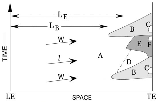
Figure 1.
Qualitative overview of LPT transition modes for a turbine cascade, taken from [16] as an adaption of [10].

Table 2.
Descriptions of the LPT transition modes for a turbine cascade.
Among the various factors that influence the loss production of a LPT, the most relevant for this study are the LSBs and wake-boundary layer interactions. Operating at low Reynolds numbers often leads to the formation of LSBs before the actual transition, which can occur in two distinct scenarios, depending on the level of FSTI: natural and bypass transition. In the first scenario, characterized by a low level of FSTI, the transition is initiated by the amplification TS waves. In the second scenario, the transition is prompted by the emergence of streamwise streaks, known as Klebanoff modes. In natural transition, small disturbances may amplify, resulting in nonlinear interactions between waves and vortices that ultimately lead to turbulence. In contrast, the bypass transition occurs when the initial disturbance amplitudes are sufficiently large to directly trigger turbulence. For intermediate FSTI values, these two modes may blend together, contributing to the transition process simultaneously, as is the case for LPT. Various methods exist to control LSBs, employing both passive and active techniques [3,4,5]. Additionally, the presence of the wake significantly influences the development of the boundary layer on the blade suction side, resulting in the generation of high level of turbulence fluctuations. The interaction between the wake and the boundary layer can advance the transition point, reduce the laminar separation bubble, and allow relaminarization.
In this study, the focus is on examining the envelope of Tollmien–Schlichting waves along the turbine blade, considering it as the initial phenomenon preceding the transition of the flow.
3. Numerical Methods Applied
3.1. Linear Stability Theory
The Linear Stability Theory is a local theory and is one of the most common methods to investigate the transition of the flow from laminar to turbulent. This method assumes parallel flow and periodicity in the other directions [17].
The first step to obtained the perturbation linearized stability equations is to define the three-dimensional Navier–Stokes equations for dimensional quantities of a viscous, incompressible flow in Cartesian coordinates. Then, the general flow variable is divided into a steady mean-flow term and an unsteady small disturbance term, as follows.
After some mathematical steps, the normal mode solutions Equation (2) for the parallel flow equations are obtained.
The normal modes represent the natural oscillation modes of the boundary layer. In this context, and are the streamwise and spanwise wave numbers, is the angular velocity, and are the eigenfunctions. When is complex while and are real, the analysis is spatial. Conversely, if is complex, it is a temporal analysis. This study employs the spatial analysis approach. The wave number is composed of two parts: a real part, which determines whether the mode is stable () or unstable (), and an imaginary part, which indicates whether the mode is damped () or amplified (). When the mode is damped, the oscillations decrease, while when the mode is amplified, the oscillations increase in space. Now, the system of linear differential equations that describe the evolution of perturbations are obtained.
where . The boundary conditions are the no-slip condition at the wall and zero disturbances in the far-wall region. These are homogeneous, leading to an eigenvalue problem. The solutions of the equations for modal functions, which satisfy boundary conditions, exist only for a particular combinations of .
The stability numerical results are presented in the neutral-stability curve. An example of this diagram is reported in Figure 2, obtained using the DEKAF and VESTA toolkits. The diagram pertains to spatial amplification theory, with the dimensional frequency (F) in Hz, plotted on the y-axis and the normalized Reynolds number () on the x-axis. As the Reynolds number increases, instability waves can be damped if they are outside the curve, remain neutral if they lie on the curve, or be amplified if they fall within it. The critical Reynolds number is the threshold below which instabilities cannot be amplified. With the linear stability theories only, the perturbation dynamics during linear stages of disturbance development is properly described. However, it is possible to correlate the linear amplification with the transition onset location observed experimentally. In particular, the method is used to obtained the disturbance amplification ratio and the N factor, Equation (4). The latter indicates the level of amplification of unstable perturbations in the boundary layer flow. The first version of this method was developed in 1956 by Van Ingen [18], with the result that the transition consistently occurred at an N-factor value of 9. Subsequently, the method progressed to , where the N-factor is calculated considering the level of free stream turbulence () [17,18]. For the LST theory, the N-factor is defined as follows:
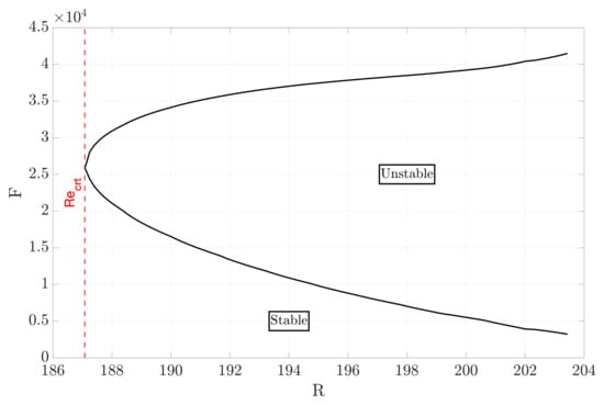
Figure 2.
Neutral stability curve with the spatial amplification theory, obtained with DEKAF and VESTA toolkits. Study case: and . Y-axis: dimensional Frequency (F) in Hz, X-axis: normalized Reynolds number (R).
In the equation provided, represents the amplification rate, and denotes the dimensionless streamwise direction.
3.2. Linear Parabolized Stability Equations
The Parabolized Stability Equations (PSEs) enable the consideration of non-parallel effects in boundary layer stability, providing a method to examine individual Fourier modes or their interactions along the streamwise direction. These equations model the propagation of disturbances over a large region and are particularly applicable to convectively unstable flows. Additionally, the PSE assumption lies in a scale separation between a slow variation of flow quantities along the streamwise direction and a strong variation along the normal-wall direction. This separation allows the disturbances to be decomposed into a slowly varying shape function and a rapidly oscillating wave part [19,20,21,22]. Finally, this study utilizes only the Linear Parabolized Stability Equations (LPSEs). One reason for this choice is that the amplification rate increases rapidly, allowing the non-linearities to be neglected, as will be highlighted in the results.
The starting point for establishing the evolution of disturbances within the boundary layer is the Navier–Stokes equations in Cartesian coordinates for compressible flows [20,22]. The general flow variable is then divided into a steady mean-flow term and an unsteady small disturbance term. Through a series of mathematical steps, the non-linear equations governing the disturbance are derived. This leads to the description of a spatially evolving two-dimensional wave with constant .
In Equation (5), is the eigenfunction and models the slowly changing profile, while described the wavelike nature of the disturbance. In particular,
where and , with the streamwise wave number. The wave component exhibits ellipticity, which is essential for describing instabilities in the form of waves, but also induces numerical instability. To address this, the oscillatory behavior of , Equation (5), is eliminated, resulting in the parabolization of the equations. Furthermore, both and vary with x, introducing ambiguity into this partition. This ambiguity proves beneficial when analyzing flows that exhibit the following two properties in the velocity profile: wavelengths and growth rates exhibit slow variations in the streamwise direction, and disturbances grow and decay as convected instabilities. Thanks to the first property, a normalization condition is specified, Equations (13)–(15), ensuring that and become slowly varying functions of x.
The subsequent step involves defining the derivatives of with respect to x as linear in and , based on the first property. This is then applied to the disturbance equation, followed by a linearization process, resulting in the following LPSE, Equation (8). To solve this equation, a marching technique is needed in the streamwise direction, such as the first or second-order backward Euler.
The L, , and are functions of the mean flow quantities and the stability parameters. Specifically,
In the given equations, is the Orr–Sommerfeld operator, accounts for the normal velocity component of the basic flow. Finally, a scalar equation is required to close the system in the LPSEs due to the parabolic nature of the eigenfunctions, which necessitates an appropriate normalization process. There are different options for the normalization:
- Base flow quantities
- Derivative of the vector of disturbances quantities
- Integral of the vector of disturbances quantities
In the equations provided, is the complex velocity profile defined as , is the complex conjugate, and is a specified location usually near the point where is maximum.
Finally, the physical growth rate, which characterizes the growth of disturbances, and the N factor can be generally quantified as follows:
3.3. Boundary Layer Profile Generation
The base flow requires the generation of boundary layer profiles, which is achieved using two numerical methods. The first method to generate the laminar boundary-layer profiles for the stability analysis uses the CFD software MISES, a commercial Euler solver developed by the Massachusetts Institute of Technology (MIT) for cascade design and analysis. This software includes capabilities for grid generation and initialization, flow analysis, result plotting, and interpretation, and provides an interactive tool for specifying design conditions [23]. The prediction of the BL transition is integrated into the laminar formulation using spatial amplification theory. Key criteria, such as the eN method [18] and the AGS (Abu-Ghanman/Shaw) criterion, are applied.
In this work, MISES is used to obtain the boundary layer properties and the inviscid flow field of the turbine blade, which serves, respectively, as a comparison and input for the second method employed to generate the BL profiles: the DEKAF toolkit. This toolkit is a boundary-layer spectral solver that provides the option to include or exclude the self-similar assumption. When the self-similar assumption is not applied, a boundary layer approach is used. The latter is the method employed in the LPT case study. Once the boundary layer profiles are generated, they serve as input into the VESTA toolkit.
Finally, the generation of the BL profiles is divided into two scenarios: the base case and the case incorporating active flow control techniques. In the latter scenario, both suction and blowing techniques are explored.
4. The Test Case SPLEEN
The transonic low-pressure turbine blade geometry from the EU program SPLEEN is utilized. The SPLEEN C1 blade profile was designed for a transonic outlet Mach number, high deflection, and low flow acceleration in the high-speed, low-Reynolds facility S-1/C of the von Karman Institute.
As depicted in Figure 3a, [24], a 13-stage axial flow compressor drives the continuous closed-loop facility of the wind tunnel, and a heat exchanger allows for maintaining the flow temperature at near ambient conditions. A vacuum pump is present, and the cascade test section is mounted in the first elbow of the loop, following the diffuser.
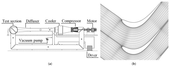
Figure 3.
(a) The VKI S1-C wind tunnel [24]. (b) Profile of the SPLEEN test case, shown with MISES mesh.
The linear cascade consists in 23 blades and the geometrical and fluid dynamics characteristics are reported in Table 3. The cascade design shown in Figure 3b has been acquired using the CFD software MISES [24]. The maximum thickness of the profile in the engine configuration is maintained, and a relatively conservative pitch-to-chord ratio is selected to reduce flow separation on the blade SS [24]. This value plays a crucial role in defining the mass flux at the inlet when analyzing the effects of active flow control techniques. Various experimental test cases were conducted in SPLEEN at and , representative of engine conditions, under both on-design and off-design scenarios. The objectives were to investigate the aerodynamics, the loss generation mechanisms, and the interactions between cavity flows, secondary flows, and wakes. The findings suggest benefits of operating at transonic outlet Mach numbers and at low Reynolds numbers. Additionally, a laminar separation bubble is present in the boundary layer on the blade profile [25,26,27,28].

Table 3.
Cascade geometry parameters, adapted from [24].
To carry out the CFD study and perform the flow stability analysis, the different flow conditions considered are defined for the main cases in Table 4. This study specifically focuses on understanding the BL modes transition phenomena at both lower and higher Mach and Reynolds numbers.

Table 4.
Flow conditions for the main cases of study.
5. Linear Stability Analysis Results
5.1. Base Flow Analysis
To perform the base flow analysis, key boundary layer properties are presented below.
- The momentum thickness, Equation (18), quantifies the momentum loss due to viscous friction between the fluid and the surface. It provides a measure of how much the boundary layer reduces the effective mass flow compared to an inviscid flow.
- The shape factor, Equation (19), characterizes the shape of the velocity boundary layer. It is defined as the ratio between displacement and momentum thickness, and it reflects the boundary layer state.
- The wall shear stress, Equation (20), directly measures the friction between the fluid and the wall. It plays a key role in determining the skin friction drag and influences heat transfer and transition phenomena.
The first property analyzed is the momentum thickness, Figure 4. This finding demonstrates that the boundary layer becomes thicker along the blade surface and is affected by both Mach and Reynolds numbers. Specifically, for a given Mach number, an increase in the Reynolds number results in a decrease in the maximum momentum thickness, suggesting that the boundary layer profiles become thinner and the viscous effects on the wall are reduced. A similar, though less marked, trend is observed when the Mach number increases for a given Reynolds number. Finally, the solid lines reach zero at a certain streamwise location due to the impending transition, which causes the BL solver to be unable to continue solving the boundary layer flow.
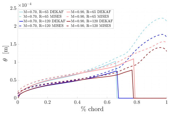
Figure 4.
Comparison of the momentum thickness for the different study cases.
This trend is also evident in the shape factors curves presented in Figure 5, where the maximum value increases as the Reynolds number rises.
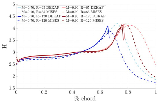
Figure 5.
Comparison of the shape factor H for the different study cases.
Finally, the wall shear stress is affected by both the Mach and Reynolds numbers, as depicted in Figure 6. Notably, all curves show a decrease in the streamwise direction due to the thickening of the boundary layer. As the Mach number increases for a given Reynolds number, the rises, driven by the enhanced compressibility of the flow. Conversely, for a fixed Mach number, an increase in the Reynolds number leads to a higher velocity gradient at the wall, resulting in an increase in along the blade surface. This increase is more marked for compared to . Towards the end of the graph, all curves converge to very low values, indicating a potential flow separation and transition.
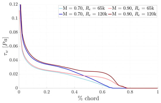
Figure 6.
Comparison of the wall shear stress for the different study cases.
In all the results presented, DEKAF (solid lines) exhibits close agreement with the outcomes from MISES (dashed lines), enabling a detailed comparison between the CFD solver and the boundary layer toolkit, up to the point of significant disturbance amplification. Finally, the solid lines vanish at a streamwise location of of the chord, depending on the Mach and Reynolds numbers, which is taken in this study as the indicator of the transition onset.
5.2. Comparison of LST and PSE Results
The stability analysis results from VESTA tool include a comparison of the physical growth rates obtained through both the method and LPSE theory, to emphasize the positive effects of the global theory on the local one.
Starting with the LST results, the physical growth rates are illustrated in Figure 7 and the N-factors in Figure 8. As the Reynolds number increases for the same Mach number, the transition point where the unstable selected mode shifts from being damped to amplified occurs earlier. Conversely, as the Mach number increases, for a given Reynolds number, this transition point is delayed, indicating that the mode remains damped over a longer streamwise distance. These results are also evident in the N-factors envelope. In fact, when the N-factor is zero, the selected modes are damped, and it begins to increase as the perturbations start to grow. The exponential shape indicates that the flow is becoming increasingly unstable, demonstrating the rapid amplification of the disturbances.
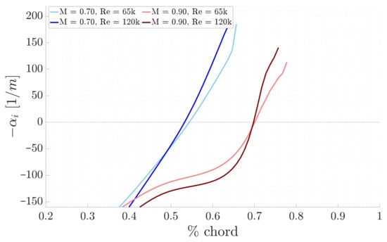
Figure 7.
Comparison of LST physical growth rates for the different study cases, with F = 25 kHz.
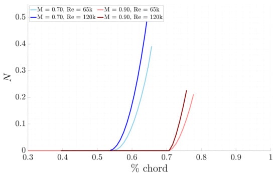
Figure 8.
Comparison of LST N-factors for the different study cases, with F = 25 kHz.
For the LPSE analysis, the physical growth rates and the N-factors are illustrated in Figure 9 and Figure 10, confirming the previous results. In fact, for a given Mach number the unstable selected mode begins to amplify earlier as the Reynolds number increases. Similarly, at higher Mach numbers, the onset of amplification occurs later. Additionally, a rapid acceleration in the amplification of the mode is observed, as expected from the global theory where local, upstream, and historical flow conditions are considered. Finally, the peaks observed after a certain streamwise location occur because the boundary layer is no longer being solved, as discussed in Section 5.1, Figure 4.
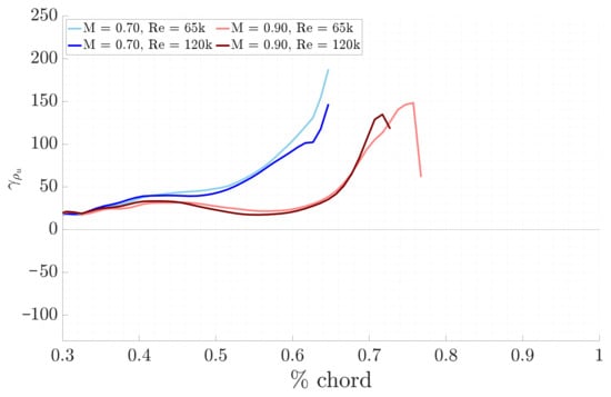
Figure 9.
Comparison of LPSE physical growth rates for the different study cases, with F = 25 kHz.
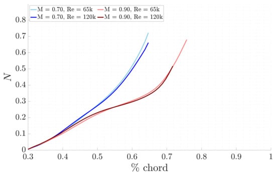
Figure 10.
Comparison of LPSE N-factors for the different study cases, with F = 25 kHz.
All these results highlight that the selected unstable mode begins to amplify much earlier on the blade suction side according to the global theory, compared to the local theory results. This is illustrated in Figure 11, where the LST results are represented by dashed lines and the LPSE results are depicted by solid lines. This discrepancy occurs because, in the LPSE, the N-factor rises immediately and reaches higher values since the instabilities are already present and amplifying when non-parallel effects are considered.
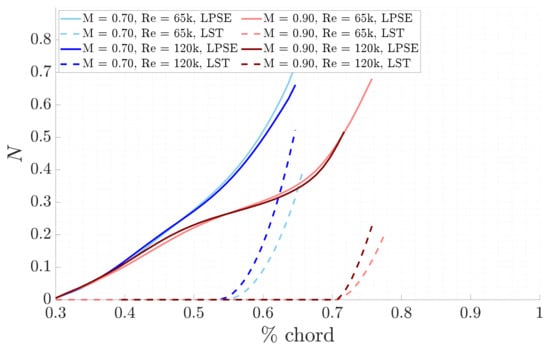
Figure 11.
Comparison of LST and LPSE N-factors for the different study cases, with F = 25 kHz.
6. The LPT Boundary Layer Transition Subject to Suction and Blowing
For this study, the effects of typical active flow control techniques on the BL transition location are investigated, specifically focusing on suction and blowing. The suction technique involves extracting part of the boundary layer flow, which thins the latter and reduces the flow momentum close to the wall. This results in accelerated residual flow and increased adherence to the wall, delaying flow separation and maintaining the laminar flow for a longer period of time. Conversely, in the blowing technique, a portion of the flow is introduced into the boundary layer, which energizes it and accelerates the flow near the wall. This promotes flow transition resulting in a more robust flow close to the wall, thereby delaying flow separation.
For the implementation of these two active flow control techniques, MISES, DEKAF, and VESTA are employed. MISES is used to analyze how the free transition point changes with the application of these techniques. DEKAF and VESTA toolkits are then used for stability analysis. Finally, the streamwise chord range where these techniques are applied in both MISES and DEKAF is . Initially, the case with and = 65,000 was studied iteratively to determine the most suitable chord range.
6.1. The Suction Ratio
To implement active flow control techniques, the suction ratio has to be defined, indicating the efficiency of suction or blowing of the flow. It is defined as the ratio between the flow rate of the suctioned fluid and the flow rate of the available fluid. In this study, the is imposed, and both the suctioned and the available mass fluxes are determined based on the definition given in MISES.
where the variables are associated with the inlet flow conditions, P is the circumferential pitch of the cascade in radians, while b and r are parameters defined in MISES. The effects of the suction and blowing on the MISES free transition point are presented in Figure 12. The upper portion illustrates the effect of blowing, while the lower portion depicts the effect of suction. The circular marker represent the base line case. As the increases in module, the free transition point for blowing occurs earlier, whereas for suction it is delayed.
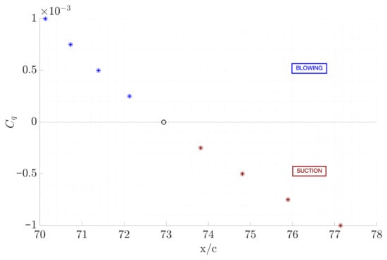
Figure 12.
Effects of suction () and blowing () techniques on the free transition point, for and , obtained with MISES.
6.2. Comparison Between LST and LPSE Analysis Results
The stability results are here shown with . First, the suction technique results are discussed. The LST physical growth rates, shown in Figure 13, show that the transition of the selected unstable mode, from being damped to amplified, occurs later compared to the respective base case. This finding is also reflected in the N-factors envelope, reported in Figure 14: the curves begin to rise exponentially as the perturbation starts to grow, but later than the respective base case. The LPSE results, in Figure 15 and Figure 16, further support this observation.
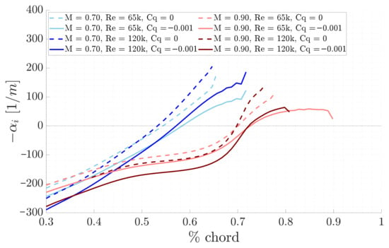
Figure 13.
Comparison of LST physical growth rates between suction and base line for the different study cases.
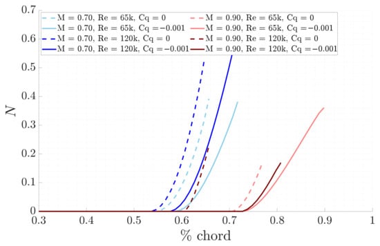
Figure 14.
Comparison of LST N-factors between suction and base line for the different study cases.
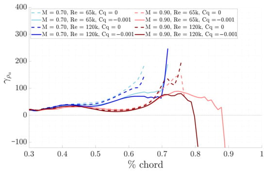
Figure 15.
Comparison of LPSE physical growth rates between suction and base line for the different study cases.
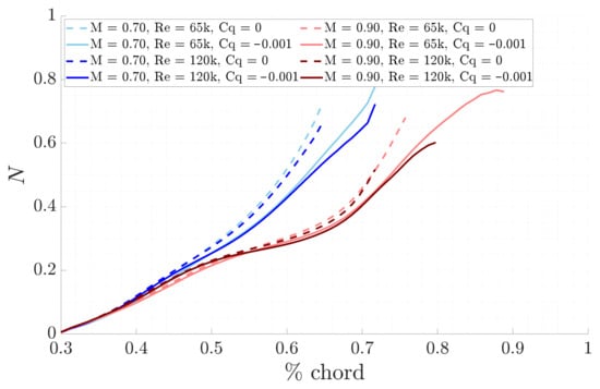
Figure 16.
Comparison of LPSE N-factors between suction and base line for the different study cases.
Now, the effects of the blowing technique are presented. The LST physical growth rates shown in Figure 17 indicate that the transition of the selected unstable mode, from being dumped to amplified, occurs earlier compared to the respective base case, as expected from theory. This is further supported by the N-factors envelope, as illustrated in Figure 18, where the curves remain at zero, while the selected unstable mode is damped and begins to rise exponentially when it starts to amplify, occurring earlier than in the respective base case. The LPSE physical growth rates and N-factors, illustrated in Figure 19 and Figure 20 respectively, confirm these findings. In fact, they demonstrate both a greater amplification of the unstable selected mode and an earlier onset of maximum increase, compared to the respective base cases. Additionally, an immediate amplification increase compared to the local results is observed, as expected from the effects of non-parallel flow.
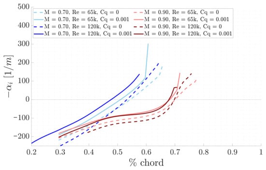
Figure 17.
Comparison of LST physical growth rates between blowing and base line for the different study cases.
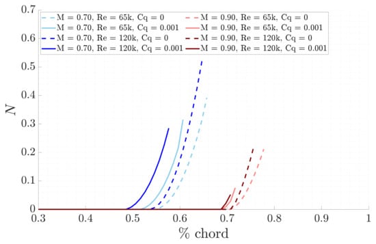
Figure 18.
Comparison of LST N-factors between blowing and base line for the different study cases.
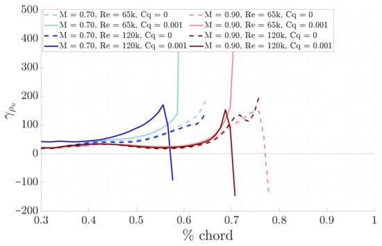
Figure 19.
Comparison of LPSE physical growth rates between blowing and base line for the different study cases.
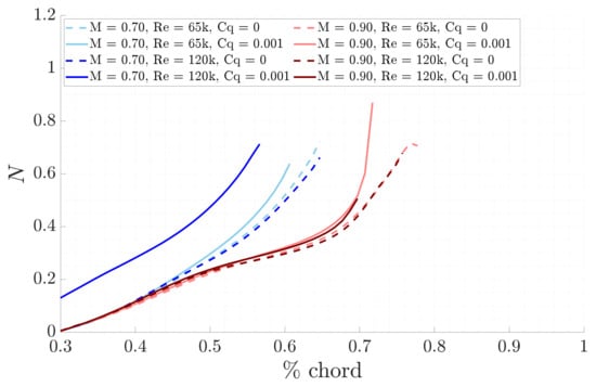
Figure 20.
Comparison of LPSE N-factors between blowing and base line for the different study cases.
Finally, for both suction and blowing, the observations regarding the effects of high and low Mach numbers and Reynolds numbers are consistent with those of the baseline and align with theoretical expectations. Furthermore, the LPSE growth rates and N-factors show significant oscillations and peaks, as beyond a certain streamwise position, the boundary layer solver is unable to accurately resolve the BL flow, which experiences extremely high amplification. This phenomenon, previously discussed in Section 5.1, Figure 4 for the baseline case, is thus also observed in the suction and blowing techniques.
7. Conclusions
This study investigated the transition from laminar to turbulent boundary layer flow in a Low-Pressure Turbine. The objective was to assess the effectiveness of Linear Stability Theory (LST) and Linear Parabolized Stability Equations (LPSEs) for LPT applications compared to the conventional method. While DNS effectively captures early transition stages, it is too expensive. LES, though an alternative, remains costly and not highly effective, while RANS methods are inadequate for these studies. Moreover, other existing software, like MISES, rely on empirical correlations. Thus, LST and LPSE theories are particularly advantageous, as they capture the early relevant natural transition scales while maintaining a low computational cost.
This research utilizes the LPT blade geometry from the EU program SPLEEN, conducted at the von Karman Institute for Fluid Dynamics. Numerically, three toolkits are used: MISES, DEKAF, and VESTA. MISES was utilized to obtain the viscous and inviscid flow field along the blade for the different flow conditions. The DEKAF toolkit is a BL solver, providing the BL profiles. Finally, the output from DEKAF served as input for the VESTA toolkit, which performed stability analysis using both LST and LPSE theories. This analysis was further extended with the implementation of two active flow control techniques: suction and blowing. The goal was to study the effects of these techniques on the transition location.
The main findings confirm that both local and global stability analyses effectively capture and study the early stages of transition.
- The LST analysis shows that the growth rate and the N-factor envelope of the selected unstable modes in the BL flow remain damped until a certain point, after which they amplify. This indicates that perturbations are growing along the blade profile, leading to flow separation and transition. For a given Mach number, as the Reynolds number increases, the amplification of the unstable mode occurs earlier. Conversely, the transition mode occurs later at a higher Mach number.
- The LPSE results align with these observations, further validating the expected boundary layer behavior. Moreover, they highlight the influence of local, upstream, and historical effects, which lead to an earlier amplification of unstable modes compared to LST predictions.
- The final results focus on the active flow control techniques, suction and blowing, including a comparison with the respective base cases. As expected, suction helps the flow remain laminar for a longer period, causing the selected unstable modes to start amplifying later than in the corresponding baseline case. Conversely, blowing accelerates the transition to turbulence, leading to an earlier amplification of the selected modes.
All these results align with the expected physical behavior and initial findings, and they provide a quantitative description of trends in terms of frequencies, amplitude growth, and wavelengths. The suitability of the two stability theories is thus confirmed, establishing a foundation for their future validation to ensure their accuracy and reliability.
However, some limitations have been identified. The use of linear theories is constrained by their ability to capture only the early stages of transition, focusing on small perturbations. Consequently, these theories may not accurately represent flow dynamics in the presence of high instability. Another limitation is that the DEKAF toolkit is specifically designed for analyzing stable flows, rendering it unable to capture flow separation and transition. Consequently, in both baseline cases and those involving active flow control techniques, the LPSE physical growth rates and N-factors results exhibit peaks and oscillations. To address these limitations, MISES is employed to gain a better understanding of the CFD conditions and provide a base for comparison.
The present work establishes a foundation for further examination of boundary layer transition phenomena in LPTs using fast and cost-effective approaches such as the proposed methodology, having resolved the scale issue. By delving deeper into this area, the goal is to optimize the design and efficiency of the LPT. While initial steps have been taken with active flow control techniques, further investigation is needed to explore the impacts of cooling, heating, and the wake–boundary layer interaction.
Author Contributions
Conceptualization, A.F. and F.E.; methodology, A.F.; formal analysis, A.F.; investigation, A.F.; writing—original draft preparation, A.F.; writing—review and editing, A.F.; supervision, F.E.; project administration, F.E.; funding acquisition, F.E. All authors have read and agreed to the published version of the manuscript.
Funding
The APC was funded by Euroturbo.
Data Availability Statement
The original contributions presented in this study are included in the article. Further inquiries can be directed to the corresponding author.
Conflicts of Interest
The authors declare no conflicts of interest.
Abbreviations
The following abbreviations are used in this manuscript:
| CFD | Computational Fluid Dynamics |
| BL | Boundary Layer |
| FSTI | Free Stream Turbulence Intensity |
| DNS | Direct Numerical simulations |
| LES | Large Eddy Simulations |
| URANS | Unsteady Reynolds-Averaged Navier–Stokes |
| TS | Tollmien-Schlichting |
| LPT | Low-Pressure Turbine |
| SPLEEN | Secondary and Leakage Flow Effects in High-SPeed Low-PrEssurE TurbiNes |
| DEKAF | Digits by Ethan, Koen, Alex, and Fernando |
| VESTA | von Karman Institute Extensible Stability and Transition Analysis |
| LST | Linear Stability Theory |
| LPSE | Linear Parabolized Stability Equations |
| MISES | Multiple blades Interacting Streamtube Euler Solver |
| LKE | Laminar Kinetic Energy |
| URANS | Unsteady Reynolds-Averaged Navier-Stokes |
| TRACE | Turbomachinery Research Aerodynamic Computational Environment |
| AGS | Abu-Ghanman/Shaw |
| MIT | Massachusetts Institute of Technology |
| LE | Leading Edge |
| TE | Trailing Edge |
| SS | Suction Side |
| LSBs | Laminar Separation Bubbles |
References
- Drela, M. MISES Implementation of Modified Abu-Ghannam/Shaw Transition Criterion; MIT Aero-Astro: Cambridge, MA, USA, 1998. [Google Scholar]
- Reshotko, E. Paths to Transition in Wall Layers. In Advances in Laminar-Turbulent Transition Modeling, 1-8; von Karman Institute for Fluid Dynamics: Sint-Genesius-Rode, Belgium, 2008. [Google Scholar]
- Hosseinverdi, S.; Fasel, H.F. Laminar-turbulent transition in a laminar separation bubble in the presence of free-stream turbulence. Procedia IUTAM 2015, 14, 570–579. [Google Scholar] [CrossRef][Green Version]
- Borgmann, D.; Fasel, H.F.; Hosseinverdi, S. Investigation of Laminar Separation Bubbles Using Experiments, Theory and DNS. In Proceedings of the AIAA AVIATION Forum, Virtual Event, 2–6 August 2021. [Google Scholar][Green Version]
- Jahanmiri, M. Laminar Separation Bubble: Its Structure, Dynamics and Control; Chalmers University of Technology: Göteborg, Sweden, 2011. [Google Scholar][Green Version]
- Zhang, W.; Zou, Z. Large eddy simulations of periodic wake effects on boundary-layer transition of low-pressure turbine cascades. AIP Adv. 2023, 13, 025128. [Google Scholar] [CrossRef]
- Stieger, R.D. The Effects of Wakes on Separating Boundary Layers in Low Pressure Turbines; Cambridge University Engineering Department: Cambridge, UK, 2002. [Google Scholar]
- Ferreira, T.S.C. Boundary Layer Transition and Convective Heat Transfer of the High-Pressure Turbine Vane LS89. von Karman Institute for Fluid Dynamics, Université Catholique de Louvain; Ottignies-Louvain-la-Neuve, Belguim, 2021. Available online: https://dial.uclouvain.be/pr/boreal/object/boreal:248082 (accessed on 22 July 2025).
- Wissink, J.; Rodi, W.; Michelassi, V. Analysis of DNS and LES of Flow in a Low Pressure Turbine Cascade with Incoming Wakes and Comparison with Experiments. J. Flow Turbul. Combust. 2002, 69, 295–329. [Google Scholar]
- Halstead, D.E.; Wisler, D.C.; Okiishi, T.H.; Walker, G.J.; Hodson, H.P.; Shin, H.-W. Boundary Layer Development in Axial Compressors and Turbines. J. Turbomach. 1997, 119, 114–127. [Google Scholar] [CrossRef]
- Groot, J.K.; Mirò Mirò, F.; Beyak, S.E.; Moyes, A.J.; Pinna, F.; Reed, H.L. DEKAF: Spectral Multi-Regime Basic-State Solver for Boundary-Layer Stability. In Proceedings of the Fluid Dynamics Conference, Atlanta, GA, USA, 25–29 June 2018. [Google Scholar]
- Zanus, L. Project Report: Analysis of a Compressible Boundary Layer Flow by Means of Parabolized Stability Calculation; von Karman Institute of fluid dynamics: Rhode Saint Genèse, Belgium, 2016. [Google Scholar]
- Padilla Montero, I. Analysis of the Stability of a Flat-Plate High-Speed Boundary Layer with Discrete Roughness. Ph.D. Thesis, von Karman Institute for Fluid Dynamics; École Polytechnique de Bruxelles, Sint-Genesius-Rode, Belgium, 2021. [Google Scholar]
- Pinna, F. Numerical Study of Stability of Flows From Low to High Mach Number. Ph.D. Thesis, von Karman Institute for Fluid Dynamics-Università di Roma “La Sapienza”, Sint-Genesius-Rode, Belgium, 2012. [Google Scholar]
- Fischer, A.; Eulitz, F. Investigation of the laminar-turbulent transition mechanisms of low-pressure turbine boundary-layers with linear stability theories. In Proceedings of the 16th European Turbomachinery Conference, Paper No. ETC2025-217, Hannover, Germany, 24–28 March 2025; Available online: https://www.euroturbo.eu/publications/conference-proceedings-repository (accessed on 22 July 2025).
- Eulitz, F. Numerische Simulation der Instationären Strömung in Turbomaschinen; DLR Forschungsbericht: Köln, Germany, 2005. [Google Scholar]
- Mack, L.M. Boundary-Layer Linear Stability Theory; AGARD Report No. 709, Part 3; California Institute of Technology: Pasadena, CA, USA, 1984. [Google Scholar]
- van Ingen, J.L. The eN Method for Transition Prediction; Faculty of Aerospace Engineering: TU Delft, The Netherlands, 2008. [Google Scholar]
- Bertolotti, F.P.; Herbert, T. Analysis of the Linear Stability of Compressible Boundary Layers Using the PSE. In Theoretical and Computational Fluid Dynamics; Springer: Berlin/Heidelberg, Germany, 1991. [Google Scholar]
- Chang, C.-L.; Malik, M.R.; Erlebacher, G.; Hussaini, M.Y. Linear and Nonlinear PSE for Compressible Boundary Layers; Institute for Computer Applications in Science and Engineering, NASA Langley Research Center: Hampton, VA, USA, 1993. [Google Scholar]
- Bertolotti, F.P. Compressible Boundary Layer Stability Analyzed with the PSE Equations; Princeton University: Princeton, NJ, USA, 1991. [Google Scholar]
- Bertolotti, F.P. Linear and Nonlinear Stability of Boundary Layers with Streamwise Varying Properties; The Ohio State University: Columbus, OH, USA, 1991. [Google Scholar]
- Drela, M.; Youngren, H. A User’s Guide to MISES 2.63; MIT Aerospace Computational Design Laboratory: Cambridge, MA, USA, 2008. [Google Scholar]
- Simonassi, L.; Lopes, G.; Gendebien, S.; Torre, A.F.M.; Lavagnoli, S. An experimental test case for transonic low-pressure turbine-Part I: Rig design, instrumentation and experimental methodology. In Proceedings of the ASME Turbo Expo 2022 Turbomachinery Technical Conference and Exposition, Rotterdam, The Netherlands, 13–17 June 2022. [Google Scholar]
- Lopes, G.; Simonassi, L.; Lavagnoli, S. Impact of unsteady wakes on the secondary flows of a high-speed low-pressure turbine cascade. In Proceeding of the 15th European Conference on Turbomachinery Fluid Dynamics and Thermodynamics, Budapest, Hungary, 22 September 2023. [Google Scholar]
- Simonassi, L.; Lopes, G.; Lavagnoli, S. Time-averaged aerodynamics of a high-speed low-pressure turbine cascade with cavity purge flow and unsteady wakes. In Proceedings of the ASME Turbo Expo 2023 Turbomachinery Technical Conference and Exposition GT2023, Boston, MA, USA, 26–30 June 2023. [Google Scholar]
- Simonassi, L.; Lopes, G.; Lavagnoli, S. Effects of periodic incoming wakes on the aerodynamics of a High-Speed low-pressure turbine. Int. J. Turbomach. Propuls. Power 2023, 8, 35. [Google Scholar] [CrossRef]
- Canepa, E.; Lengani, D.; Niliberto, A.; Petronio, D.; Simoni, D.; Ubaldi, M.; Zunino, P. Flow coefficient and reduced frequency effects on wake-boundary layer interaction in highly accelerated LPT cascade. Int. J. Turbomach. Propuls. Power 2021, 6, 32. [Google Scholar] [CrossRef]
Disclaimer/Publisher’s Note: The statements, opinions and data contained in all publications are solely those of the individual author(s) and contributor(s) and not of MDPI and/or the editor(s). MDPI and/or the editor(s) disclaim responsibility for any injury to people or property resulting from any ideas, methods, instructions or products referred to in the content. |
© 2025 by the authors. Published by MDPI on behalf of the EUROTURBO. Licensee MDPI, Basel, Switzerland. This article is an open access article distributed under the terms and conditions of the Creative Commons Attribution (CC BY-NC-ND) license (https://creativecommons.org/licenses/by-nc-nd/4.0/).