Aerodynamic Design of Wind Turbine Blades Using Multi-Fidelity Analysis and Surrogate Models ^†

Abstract

A standard approach to design begins with scaling up state-of-the-art machines to new target dimensions, moving towards larger rotors with lower specific energy to maximize revenue and enable power production in lower wind speed areas. This trend is particularly crucial in floating offshore wind in the Mediterranean Sea, where the high levelized cost of energy poses significant risks to the sustainability of investments in new projects. In this context, the conventional approach of scaling up machines designed for fixed foundations and strong offshore winds may not be optimal. Additionally, modern large-scale wind turbines for offshore applications face challenges in achieving high aerodynamic performance in thick root regions. This study proposes a holistic optimization framework that combines multi-fidelity analyses and tools to address the new challenges in wind turbine rotor design, accounting for the novel demands of this application. The method is based on a modular optimization framework for the aerodynamic design of a new wind turbine rotor, where the cost function block is defined with the aid of a model reduction strategy. The link between the full-order model required to evaluate the target rotor’s performance, the physical aspects of blade aerodynamics, and the optimization algorithm that needs several evaluations of the cost function is provided by the definition of a surrogate model (SM). An intelligent SM definition strategy is adopted to minimize the computational effort required to build a reliable model of the cost function. The strategy is based on the construction of a self-adaptive, automatic refinement of the training space, while the particular SM is defined by the use of stochastic radial basis functions. The goal of this paper is to describe the new aerodynamic design strategy, its performance, and results, presenting a case study of a 15 MW wind turbine blades optimized for specific deepwater sites in the Mediterranean Sea.

1. Introduction

Offshore wind power, which has been under increasing development in recent years, represents a key element in the evolution of renewable energy. The recurring trend is to increase the size of the rotor to capture more energy, even at lower wind speeds. While offshore wind has seen significant development globally, particularly in Northern Europe, North America, and China [1], adapting this technology to the Mediterranean region presents new challenges. For new offshore floating wind turbine (FOWT) developments, there is the challenge of adapting projects to the specific metoceanic conditions of each site. This approach is particularly important for new developments in the Mediterranean Sea, which will play a critical role in the growth of the wind sector [2], characterized by deep waters and low wind speeds. FOWTs accounted for just 0.1% of total offshore wind capacity in 2021, but this figure is expected to rise to 6.1% by 2030, with 16.5 GW of new capacity projected [1]. However, the sustainability and risks associated with this technology suffer from a lack of reference data, wind measurements, and industrial experience, compounded by the high expected Levelized Cost of Energy (LCOE) [3,4].

Recent advancements in optimization techniques have significantly improved the design of new reference wind turbines (RWTs). One of the strategies used is to minimize the LCOE, employed as a multidisciplinary objective function [5,6,7]. Optimization algorithms, such as gradient-based methods, are widely applied to determine the optimal blade geometry, airfoil shape, and material distribution [8,9,10,11]. These optimization tools have contributed to the design of recent RWT such as NREL-5MW [12], DTU-10MW [13], and IEA-15MW models [14], which have driven offshore wind research and development studies in recent years. However, they are optimized for conditions in Northern Europe and North America, where wind speeds and ocean conditions differ significantly from those in Mediterranean waters.

Unlike regions with stronger and more uniform winds, the Mediterranean’s moderate wind speeds require rotor designs capable of operating efficiently in these lower wind regimes while also handling the complexities of floating platform motion. This introduces additional challenges in scaling rotor sizes and optimizing blade designs for FOWTs. To address these challenges, a shift away from traditional design approaches is necessary.

This paper presents a proposal for an optimization framework aimed at designing wind turbine blades tailored for the winds of the Mediterranean Sea. Using a multi-fidelity approach, the framework integrates numerical models of varying fidelity, balancing the need for sustainable computational costs with the accuracy required to solve complex non-linear aspects. The aim is to develop a design framework that can handle a multi-disciplinary context (the FOWT design and simulation), maintaining high accuracy in modeling each different physical and technical aspect while ensuring sustainable computational cost. The case study presented here focuses on a single-objective optimization to establish a baseline, reserving the multi-objective capabilities for future studies.

Multi-fidelity modeling has become an essential approach in optimizing complex engineering systems, as it allows for the integration of models with different levels of accuracy and computational cost. Studies such as those by Forrester et al. [15] and Fernández-Godino et al. [16] have demonstrated the benefits of combining multiple fidelity levels in engineering optimization. These studies highlight the potential to significantly reduce computational costs while maintaining predictive accuracy. Similarly, more recent studies, such as that by Pellegrini et al. [17], have shown the effectiveness of multi-fidelity frameworks in addressing noise evaluations and enhancing performance optimization. The multi-fidelity strategy defined here involves the use of Computational Fluid Dynamics (CFD) simulations to compute accurate blade section force coefficients, while a Blade Element Momentum Theory (BEMT) simulation is employed to evaluate rotor performance, maintaining reasonable computational costs compared to full-order simulation methods.

The method is also designed to minimize the number of full-order model calls required to accurately predict the aerodynamic aspects needed to evaluate the design cost function (e.g., the power production of a new design). A Surrogate Model (SM) is defined and trained for this purpose, based on Stochastic Radial Basis Functions (SRBFs) [18], and a self-adaptive training dataset is developed to optimize the training space and reduce computational effort.

SMs, such as SRBFs, are frequently employed in optimization tasks to approximate the performance of complex engineering systems with reduced computational cost. Forrester et al. [19] provide a comprehensive guide to the practical application of surrogate modeling in engineering design, emphasizing their effectiveness in approximating expensive simulations. In this study, we use a method based on SRBF (inspired by [18]), applied here in a single-fidelity configuration for the full-order model. The implementation, however, allows for a multi-fidelity approach based on hierarchical fidelity correction, which enables the use of different fidelity levels during SM training. This method relies on additive corrections to account for discrepancies between low- and high-fidelity data. An alternative method is co-Kriging [20], which is well-known for its ability to integrate multi-fidelity data through covariance modeling. However, this method requires extensive covariance matrix computations and hyperparameter tuning. In contrast, the SRBF-based approach adopted in this work avoids the need for assembling and inverting large covariance matrices, significantly reducing computational overhead compared to full covariance modeling. Consequently, it offers improved efficiency and robustness, particularly in scenarios with noisy or sparse data, which are common in wind turbine optimization studies. Furthermore, the SRBF-based approach can further reduce computational costs through self-adaptive design-of-experiment (DOE) selection, making it particularly well-suited to the framework presented here. The chosen optimization algorithm benefits from being able to perform a large number of evaluations of the cost function through the SM. This allows for the use of optimization algorithms suitable for complex and highly non-linear problems.

Genetic algorithms (GAs) are particularly well-suited for optimization problems, where conflicting design criteria need to be balanced. Tamaki et al. (1996) [21] and Konak et al. (2006) [22] provide a comprehensive overview of how GAs have been successfully applied to engineering optimization problems, highlighting their ability to efficiently explore large and complex design spaces. The flexibility of GAs enables them to explore trade-offs between conflicting objectives, such as maximizing aerodynamic efficiency while maintaining structural integrity. However, as GAs are often slow to converge, the integration of a SM helps the process, allowing for the use of large populations and a large number of epochs, making their application feasible for complex design tasks.

The case study presented in this paper uses the DTU FFA-W3 series and the baseline IEA 15 MW as reference turbines, attempting to obtain new designs for Mediterranean wind conditions. Although the implemented optimization algorithm allows us to account for multiple design targets, e.g., aerodynamic efficiency, structural integrity, and control, in this preliminary study, the optimization is framed as a single-objective design problem, focusing on maximizing Annual Energy Production (AEP) to perform an initial aerodynamic optimization. The input parameters include twist, chord, and airfoil thickness, which are used to compute the AEP function as these variables vary. This function is then incorporated as the objective for optimization within the GA.

This article is a revised and expanded version of our paper [23], which was presented at the 16th European Turbomachinery Conference. The paper is organized as follows: Section 2 describes the modeling framework employed in this study, detailing the integration of the application of SMs to the design strategy and the optimization algorithms used. Section 4 explores the computational tools and numerical models used in this first application. Section 5 presents the results of the optimization process, highlighting the enhancements in blade performance and efficiency. This section also discusses how the design meets the specific challenges posed by Mediterranean conditions. Finally, Section 6 summarizes the key findings of this study and suggests areas for future research.

2. Methodology

The optimization and simulation framework is applied here to a case study of wind turbine blade design aimed at maximizing the Annual Energy Production (AEP) by tailoring blade geometries to specific environmental conditions, such as the low-wind and deep-water characteristics of the Mediterranean Sea. Although the overall design process of a wind turbine involves the interaction of various critical aspects beyond pure aerodynamics and power production, such as structural loads, control systems and strategies, foundation dynamics, materials, and costs, this paper reports on an initial framework focusing on the aerodynamic design of the blade. This groundwork is intended to be extended to a more comprehensive analysis framework in future developments.

The first step is the selection of the target quantity to optimize, followed by the definition of the cost function. In this example, we set the optimization problem as follows: find a parametric blade model $\mathbf{x}$ such that the share of AEP between two given wind velocities $V1$ and $V2$ is maximized. The cost function can be computed as follows:

$$AE{P}_{12}\left(\mathbf{x}\right)=\mathrm{\Delta }T{\int }_{V_1}^{V_2}P(V,\mathbf{x})f_V\left(V\right)dV$$

(1)

where $P(V,\mathbf{x})$ is the aerodynamic power of the rotor, $f_V\left(V\right)$ is the probability density function of having wind velocity V at the target site, and $\mathrm{\Delta }T$ is the period of evaluation of the energy (one year in this case).

The second step is the definition of the blade geometry parametrization. According to recent literature [8,24], the blade shape should be defined with a controlled number of parameters to avoid an excessively large variable space, which could lead to numerous saddle points or require an unfeasible number of cost function evaluations during the optimization procedure. The blade geometry is therefore defined using a space with a limited number of control parameters, augmented by smooth interpolating functions. As per common practice, the blade is defined by specifying 1D span-wise functions for the cross-sectional twist angle $\theta$, chord length c, and maximum section thickness. Each function is represented by a cubic B-spline, where the control points serve as the optimization variables. The approach is verified by showing that the calculated $AE{P}_{12}$ using the spline-based geometry, compared to the original blade configuration, exhibits only a minor deviation of approximately 0.35%. The geometry is then completed by choosing airfoil shapes associated with the local thickness-to-chord ratio.

In this initial application, we assume that the dimensional thickness function is given and fixed, optimizing $\theta$ and c. This choice allows us to focus on aerodynamics, avoiding the need to optimize the blade thickness, which is primarily associated with structural load constraints. For the same reason, we chose to constrain the root and tip values of the chord function, leaving one control point at mid-span as a degree of freedom, while five control points are used to define the twist function. 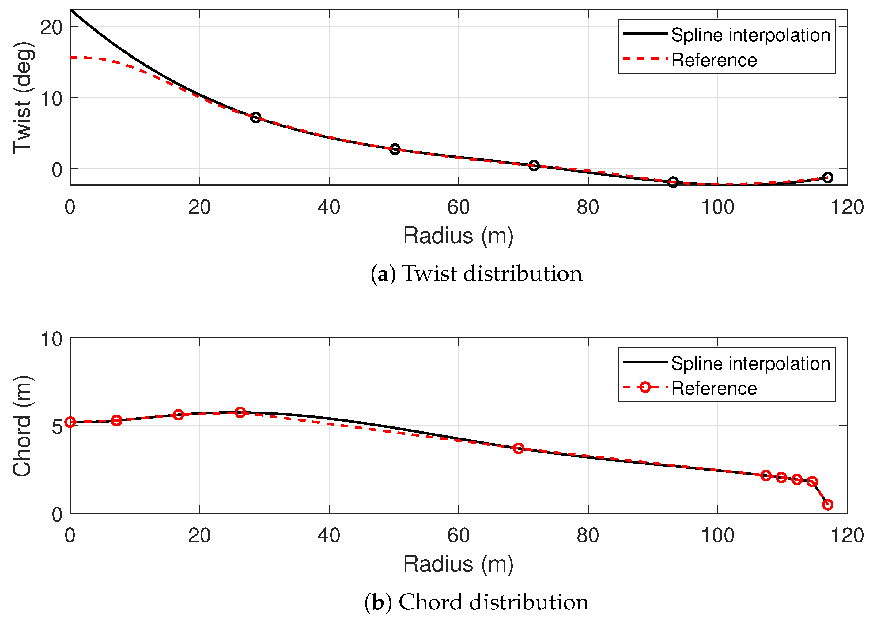Figure 1 shows the spline interpolation and control points of the $\theta$ function (Figure 1a) and the c function (Figure 1b).

Other constraints applied to the variables are simple inequality constraints that limit the range of variation to avoid unfeasible design geometries.

The optimization is conducted using a GA, chosen for its robustness in exploring complex, multi-modal design spaces. Unlike traditional gradient-based methods, which may struggle with the non-linearity present in the design space, the GA is capable of avoiding local minima and identifying globally optimal solutions. The objective function to maximize is the $AE{P}_{12}$ defined by Equation (1). The GA is initialized with a population of 200 potential solutions, each representing a different configuration of twist and chord control points. The process continues until the optimal solution is found or the improvement in $AE{P}_{12}$ falls below a predefined threshold of 1%. While GAs are effective at exploring large and complex design spaces, they do not guarantee globally optimal solutions due to their stochastic nature and reliance on heuristic search strategies. This limitation is particularly relevant when GAs are combined with SM, where the accuracy of the optimization heavily depends on the surrogate’s reliability. To address this, the SM in this study was validated against full-order model simulations, and an adaptive sampling strategy was employed to refine the SM iteratively in regions of high uncertainty. This approach, as outlined by Fernández-Godino et al. (2023) [16], ensures a balance between computational efficiency and predictive accuracy.

The evaluation of the aerodynamic power $P\left(V\right)$ for a given average wind inflow velocity V is the critical aspect, which requires reliable modeling of turbine aerodynamics. The computation module for $P\left(V\right)$ can rely on different modeling approaches, ranging from lifting-line-based models (fast but less accurate) to blade element discretization-based models, such as blade element momentum theory or actuator line models, and even geometry-resolving medium- (panel methods) to high-fidelity (CFD) methods.

In all cases, the GA will call this module thousands of times, making the optimization process extremely slow and limiting the use of higher-fidelity approaches, thus reducing their ability to capture complex and nonlinear effects.

To reduce the computational cost associated with the simulations, the direct evaluation of the cost function is replaced with a SRBF SM. The adopted approach is based on the one proposed in [18,25], where a generalized multi-fidelity meta-model was presented for design- and operational-space exploration and applied to applications such as hydrofoil optimization and ship performance prediction. The approach aims to efficiently approximate complex objective functions $f\left(x\right)$, such as $AE{P}_{12}$ in Equation (1), through a regression model based on regression functions that are defined and refined using a limited number of full-order model (FOR) computations.

In the original method, starting with low-fidelity models ${\tilde{f}}_N\left(x\right)$, which provide coarse but inexpensive predictions, higher-fidelity corrections ${ϵ}_l\left(x\right)$ are progressively added using a hierarchical error correction scheme combined with an adaptive sampling method. At each fidelity level, the difference between the model predictions and the next higher-fidelity simulations is calculated and used to update the approximation. Here, the implementation is simplified to the single level of fidelity offered by the BEMT wind turbine rotor simulation. For completeness, we report the general version of the formulation, accounting for a generic case in which low-fidelity and high-fidelity models are employed.

Consider an objective function $f\left(\mathbf{x}\right)$. This is evaluated at different fidelity levels, which correspond to numerical simulations $s_l\left(\mathbf{x}\right)$ that approximate $f\left(\mathbf{x}\right)$ with varying degrees of accuracy and computational cost. The hierarchical fidelity structure is expressed as follows:

$$s_l\left(\mathbf{x}\right)=f_l\left(\mathbf{x}\right)+N_l\left(\mathbf{x}\right),l=1,\dots ,N$$

(2)

where $s_l\left(\mathbf{x}\right)$ is the simulated response at fidelity level l; $f_l\left(\mathbf{x}\right)$ is the true but unknown function response at that fidelity level; and $N_l\left(\mathbf{x}\right)$ represents numerical noise, modeled as zero-mean uncorrelated random variables. The multi-fidelity-based approximation $\widehat{f}\left(\mathbf{x}\right)$ can be expressed as follows:

$$\widehat{f}\left(\mathbf{x}\right)={\tilde{f}}_N\left(\mathbf{x}\right)+\sum _{l=1}^{N-1}{\widetilde{ϵ}}_l\left(\mathbf{x}\right),$$

(3)

where ${\tilde{f}}_N\left(\mathbf{x}\right)$ is the SM at the lowest fidelity level and ${\widetilde{ϵ}}_l\left(\mathbf{x}\right)$ represents inter-level corrections. For ${\widetilde{ϵ}}_l\left(\mathbf{x}\right)$, we can define an SM from a training dataset, defined as follows:

$${ϵ}_l\left(\mathbf{x}\right)=s_l\left(\mathbf{x}\right)-{\widehat{f}}_{l+1}\left(\mathbf{x}\right),$$

(4)

where ${\widehat{f}}_{l+1}\left(\mathbf{x}\right)$ is the SM prediction at the next higher-fidelity level. An adaptive sampling strategy is employed to iteratively refine the SM by focusing on regions with the highest uncertainty. Using this approach, new training points are automatically added where the model exhibits the greatest uncertainty, ensuring that the SM improves its accuracy where it is most needed, thus avoiding unnecessary computations of the FOR.

The final SM is constructed using an SRBF approach, which provides both function predictions and associated uncertainties. The SRBF model is defined as follows:

$$f(y,\tau )=\sum _{j=1}^K{w}_j{\parallel y-c_j\parallel }^{\tau },$$

(5)

where K is the number of RBFs, $c_j$ represents the RBF centers, $w_j$ are the weights, and $\tau \in [1,3]\setminus \left\{2\right\}$ is the stochastic exponent. To enhance accuracy while maintaining computational efficiency, the SM is iteratively refined using an adaptive sampling approach based on the uncertainty of the SM approximation. At each iteration, the uncertainty of the approximation is evaluated on a fine grid of the parameter space by randomly varying the stochastic parameter $\tau$. A new training point is then added at the grid point (not part of the existing training set) where the uncertainty is maximum.

The performance of the geometries under the target site’s wind conditions can be generated using simulation tools of varying fidelity, ranging from low to high. In this first application, the aerodynamics of the trial blade are evaluated using a dynamic BEMT simulation with steady wind and vertical shear. The blade is discretized into a number of strips with constant 2D properties and airfoils. The aerodynamic force of each strip is interpolated from a database of tabular force coefficients versus angle of attack, obtained with high-fidelity CFD. Since each trial geometry has a different chord distribution but a fixed thickness distribution along the span, an automated process adjusts the airfoil polars to reflect changes in the blade’s thickness-to-chord ratio ($t/c$). This is achieved by dynamically selecting and interpolating the airfoil polars from the existing database based on the updated $t/c$ values of the trial blade strip. It is worth noting that the aerodynamic simulation block can be easily replaced with higher-fidelity simulation tools without interfering with the framework’s structure and logic.

3. CFD Framework for Aerodynamic Coefficient Computation

The aerodynamic optimization and the prediction of aerodynamic forces supported by BEM-based simulation strongly rely on the quality of the input in terms of the airfoil force coefficient table. In this study, the aerodynamic coefficients for the main blade sections are computed using validated CFD simulations. This framework is specifically designed to compute airfoil lift and drag polars under a range of operating conditions that extend beyond those defined in the original reference dataset, ensuring greater flexibility and accuracy in performance prediction. The framework consists of three phases: airfoil geometry processing, aerodynamic performance evaluation, and post-processing.

The geometry is defined using a MATLAB vR2023b script, generating B-spline interpolation of the airfoil from the control points taken from the reference. The script then generates a structured C-type mesh within Ansys ICEM CFD. The mesh parameters are established based on best practices identified in similar studies [26], with a domain extension of 30 chord lengths in the far field (assuming unit chord length). The mesh grid is composed of 332.000 quadrilateral cells, providing good resolution to accurately capture the flow characteristics around the airfoil. The minimum wall distance is set to $2.5\times {10}^{-6}$ m, ensuring a $y^{+}<1$ criterion for accurate near-wall turbulence modeling for all the Reynolds number considered. The turbulence intensity was set at 0.1%, with a turbulent length scale of 0.2 m at the inflow boundary. The boundary conditions for the simulations were as follows: (i) the inlet was defined as a velocity-inlet with a fixed value depending on the Reynolds number and the angle of attack, while the outlet was defined with a outflow freestream condition; (ii) the airfoil surface was modeled with a no-slip wall condition. The aerodynamic performance of each airfoil, within a range of angles of attack from $-15°$ to $25°$ (21 in total), is evaluated using RANS simulations in Ansys Fluent v22R2, using the standard $k-\omega$ SST turbulence model.

Simulations are initialized using a hybrid initialization approach and solved employing a steady-state solver until residuals achieve a convergence criterion of ${10}^{-11}$ across all equations or the solver reaches the maximum number of 2000 iterations.

The aerodynamic analysis includes simulations at three Reynolds numbers ($6.0\times {10}^6$, $9.0\times {10}^6$, and $18.0\times {10}^6$), corresponding to the expected operational range of a 15 MW wind turbine blade. The simulation framework is validated by comparing the results with reference aerodynamic data taken from the IEA 22 MW turbine dataset at a specific Reynolds number.

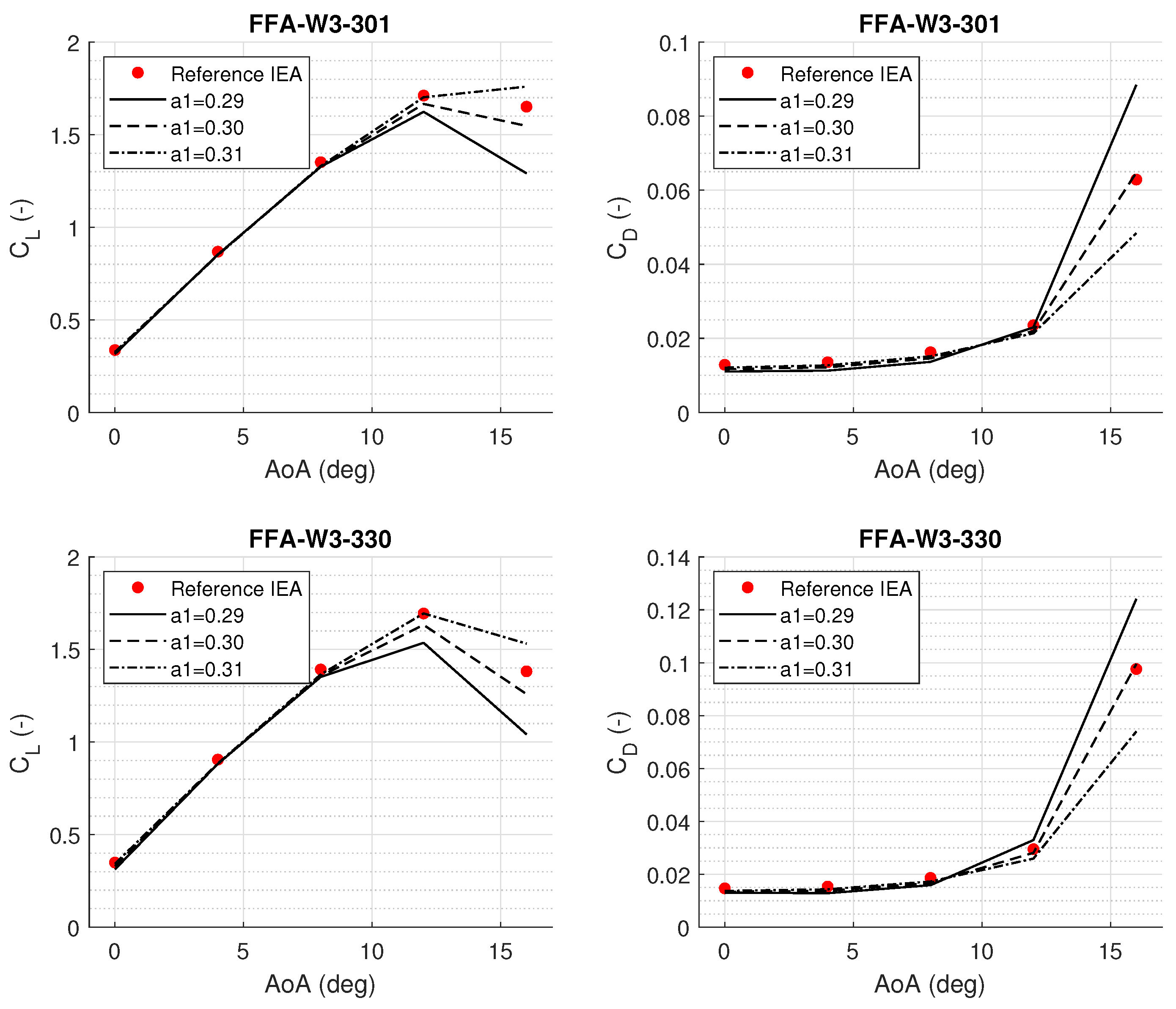
A dedicated sensitivity analysis was conducted on the turbulence model parameters. In particular, the standard $k-\omega$ SST model was tested with different values of the blending constant $a_1$. Three configurations were tested with $a_1=0.29, a_1=0.30$, and $a_1=0.31$ in order to identify the value yielding the best agreement with the reference data for a limited range of angle of attack $(0,4,8,12,16°)$. The outcomes of this comparison are illustrated in Figure 2, where the lift coefficient $\left(c_l\right)$ and drag coefficient $\left(c_d\right)$ are plotted against the angle of attack (AoA) for two different airfoils of the set, namely the FFA-W3-301 and FFA-W3-330.

The simulations here were performed using Reynolds numbers of $Re=18.0\times {10}^6$ for FFA-W3-301 and $Re=17.0\times {10}^6$ for FFA-W3-330, matching the reference IEA 15MW dataset to enable a direct comparison. The sensitivity analysis shows that the $a_1$ parameter in the k-$\omega$ SST turbulence model significantly affects the predicted $c_l$ and $c_d$ coefficients, particularly in the post-stall region. For FFA-W3-301, the setting $a_1=0.30$ yields the best agreement with the reference lift data across the full angle of attack range and was therefore selected for further calculations. In contrast, for FFA-W3-330, the configuration with $a_1=0.31$ most accurately reproduces the reference lift curve and was chosen accordingly. Although some deviations in drag predictions persist at high angles of attack, the configurations that provided the most accurate lift modeling were prioritized for both profiles. This study was repeated for all the reference airfoils, finding a best-fitting value of $a_1$.

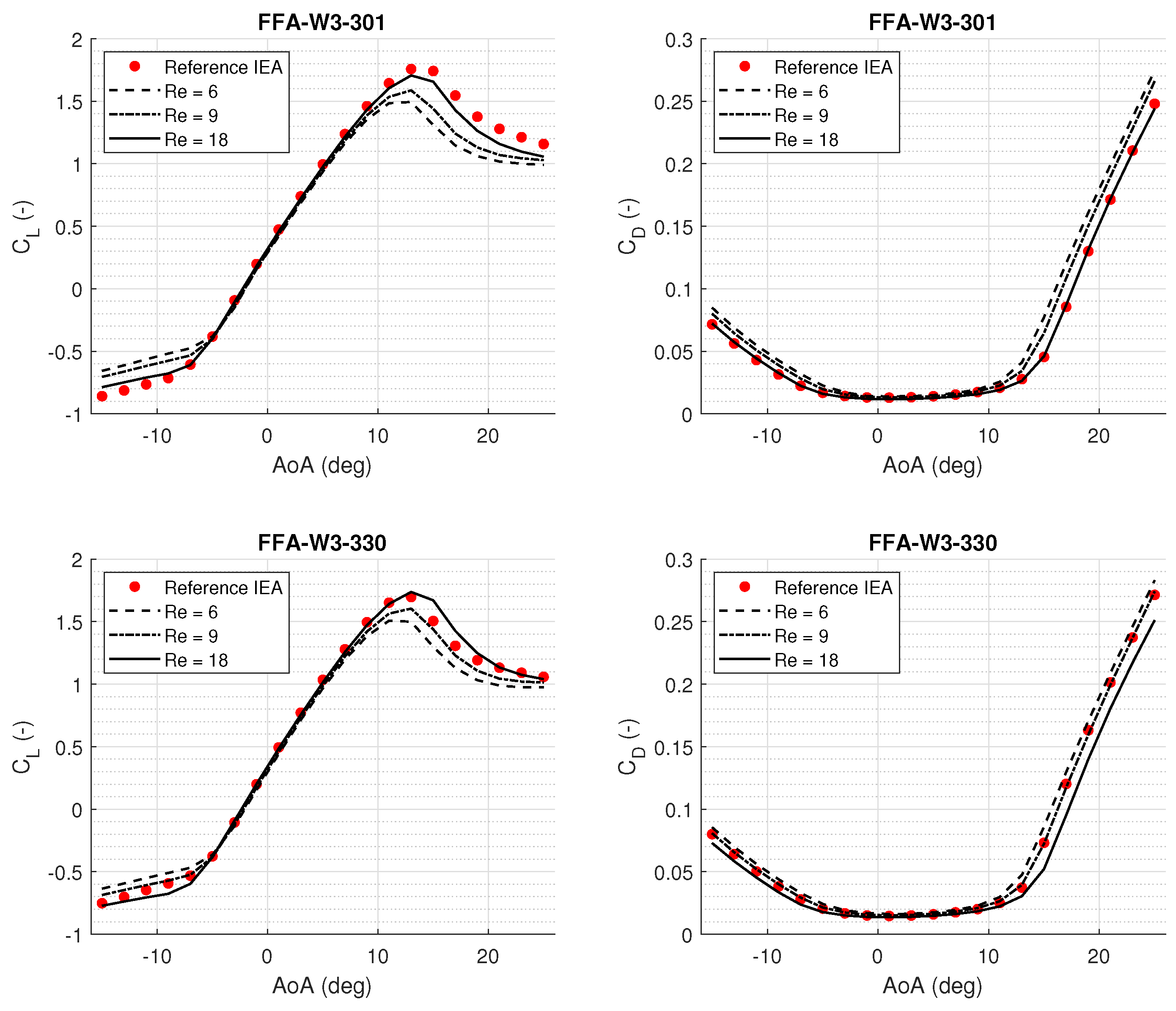
Having verified the CFD setup for each airfoil, it is possible to proceed with the production run for lower Reynolds numbers. CFD-generated aerodynamic force coefficients are shown in Figure 3, showing higher lift and reduced drag at higher Reynolds numbers, especially near stall and post-stall regions.

4. Test Case Definition

As a test case, we chose to optimize a 15MW horizontal-axis wind turbine design for IEC Class III [14], suitable for the wind conditions mainly found in the Mediterranean Sea. Accurate predictions of metocean conditions are crucial to the design of offshore turbines, as they affect energy production estimates and assessments of extreme and cyclic loading in compliance with IEC61400 standards. Significant meteorological data is available through European initiatives, including satellite-based measurement campaigns [27] and databases generated from numerical re-analyses using mesoscale models [28].

The metocean conditions were thoroughly analyzed in a preliminary survey conducted within the “NOSTRUM—Optimizing floating offshore wind turbines for use in the Mediterranean Sea” project [29], where a survey covered several potential offshore sites in the Mediterranean Sea. The wind data were extracted from the ERA5 reanalysis database [30], which provides hourly wind speed data at 100 m above mean sea level for the Mediterranean region over a 20-year period (2003–2022). For each selected site, a Weibull probability density function (PDF) was fitted to the data to model the wind speed distribution at these locations.

Assuming a hub height of 150 m, a power law with an exponent of 0.12 [31,32] was chosen to define the wind vertical profile used in the rotor performance simulation. This approach provided realistic wind data for use in blade design under Mediterranean conditions, indicating that focusing on an IEC Class III turbine is a possible target due to the moderate wind speeds.

The computation of blade aerodynamics is performed using AeroDyn.v15 [33], an open-source dynamic BEMT-based solver. The blade is divided into 50 elements along its span, and for each blade element, a full AoA range table of aerodynamic coefficients is given.

As the reference case and initial design, we chose the IEA-15-240-RWT [14]. In this way, we focused only on the aerodynamics of the blades, assuming the hub, tower, nacelle, electric generator, and other auxiliary structures remain unaltered. The idea is to replace the original rotor and revamp the machine with a newly optimized rotor design tailored to the target wind class. The hub height of the turbine is 150 m, with a hub radius of 3.97 m, and the optimal tip-speed ratio is set to 9. The shaft tilt and precone angles are set to −6^∘ and −4^∘, respectively, as in the reference design.

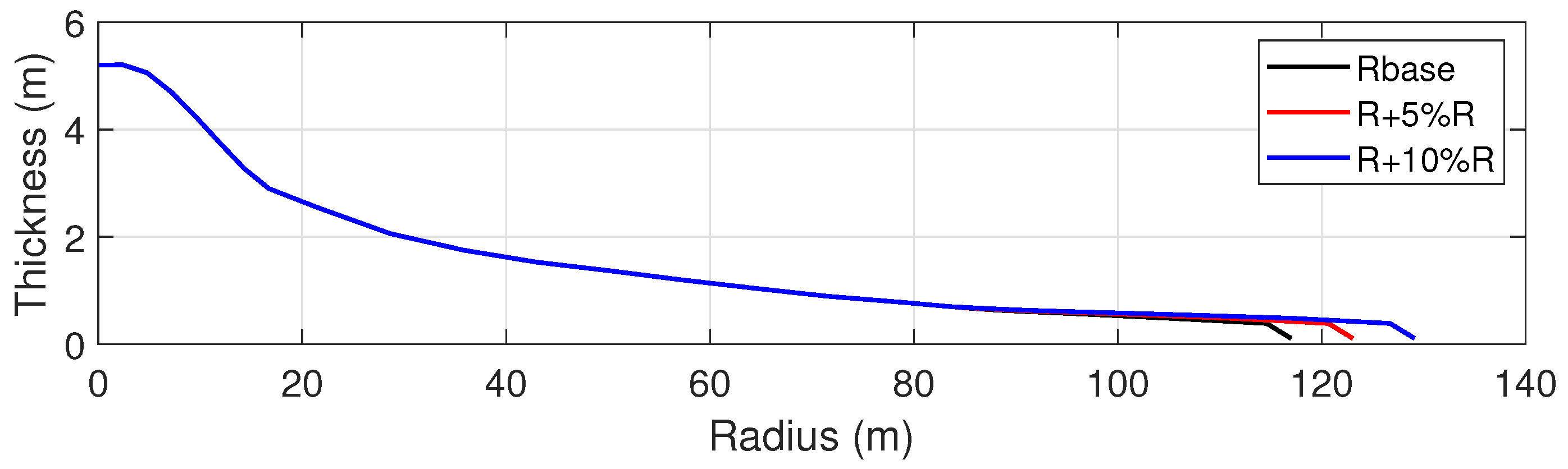
The work also includes a parametric study to evaluate possible designs with different rotor radii, allowing for the exploration of aerodynamic loading and rotor power densities, with an aim to improve the rotor’s energy capture potential, particularly at lower wind speeds. The case study defines three different targets: one with the same blade span as the reference turbine (Design 1), one with a 5% increased radius (Design 2), and one with a 10% larger rotor diameter (Design 3).

A scaling procedure is applied to increase the rotor size, assuming the same thickness function up to the point where the thickness-to-chord ratio reaches 21%. From this point onward, the span is extended using a scaling factor ($SF$) that accounts for the rotor radius:

$$SF=\alpha ·{\displaystyle \frac{R}{h}}+1$$

(6)

where $\alpha$ represents the percentage increase needed in rotor diameter, R is the rotor radius, and h is the blade section length being scaled. This provides a smooth extension of the blade radius without altering the aerodynamic profile in the root area, where less energy is extracted (Figure 4).

As reported in Section 2, the design space vector is defined by 6 control points: 5 for the twist span-wise spline function distribution, and 1 for the chord span-wise spline function distribution, located at $r/R$ = 0.59. (i) fixed root and tip control points of the chord distribution to constrain the maximum and minimum chord values; (ii) upper and lower bounds for $\mathbf{x}$, defined as $[0.19,-3.29,-4.62,-5.97,-4.24,2.7]<\mathbf{x}<[14.19,8.76,5.49,2.20,1.76,4.7]$; (iii) the maximum cross-sectional thickness is fixed and equal to the reference case.

This assumption reflects the focus of this study on aerodynamic optimization, with the primary objective of maximizing $AE{P}_{12}$. By fixing the thickness distribution, the analysis isolates the aerodynamic performance improvements achievable through variations in twist and chord distributions. This simplification allows the SM and GA framework to focus exclusively on aerodynamic factors while maintaining computational efficiency. Despite the fixed blade thickness distribution, the framework dynamically adjusts airfoil sectional properties based on the optimized blade geometry. As the chord length (c) varies during optimization, the relative thickness ($t/c$) of each section is dynamically updated, ensuring that the sectional properties and aerodynamic coefficients adapt to the new geometry. The airfoil database consists of 50 distinct profiles corresponding to the baseline blade’s elements; for intermediate values, linear interpolation is applied. This approach allows us to maintain the airfoil family, having sectional properties that are not constant but evolving according to the geometric changes introduced during the optimization process. It is recognized that the fixed blade thickness distribution does not account for structural constraints, such as bending stresses or deflection limits, which are critical for the feasibility of optimized designs. Future work will address these limitations by integrating structural considerations into a multi-objective optimization framework.

The SM is trained using data generated from aerodynamic simulations conducted with the AeroDyn.v15 module [33,34]. AeroDyn.v15 calculates the power for three different uniform wind speeds in the range of $V_1$ = 4 m/s to $V_2$ = 9 m/s, generating a discretization of the power curve for each blade design. A second-order spline interpolation of the power curve is then used in the integration of $AE{P}_{12}$ according to Equation (1). These values, along with the associated design variables $\mathbf{x}$, form the training data for the SM.

The adaptive sampling strategy employed in the SM training identifies regions in the design space where the model’s predictions are less reliable and adds new training points in those areas. This process begins by generating a uniform grid of potential design configurations based on the upper and lower bounds for the twist and chord control points. Each point in the grid corresponds to a unique combination of twist and chord values, ensuring evenly spaced exploration of the design space. The process continues by incrementing the grid resolution for a maximum number of iterations set by the authors or stops when it reaches a defined tolerance value, which is three orders of magnitude smaller than the computed $AE{P}_{12}$. Once trained and validated, the SM is integrated into the GA optimization framework. The optimization process refines the aerodynamic performance of a wind turbine blade by optimizing its twist and chord distributions.

The GA is implemented in MATLAB R2024a with a population size of 200, a mutation rate of 0.01, and a crossover fraction of 0.8. The algorithm is configured to run for 100 generations, or until the improvement in the objective function falls below 1% over five successive generations. The optimization process begins by initializing the design variables—twist and chord distributions at key control points along the blade span—using perturbed values relative to the reference geometry. The GA iteratively refines these variables, using the SM to evaluate the aerodynamic performance of each candidate design. By minimizing the computational expense of direct aerodynamic simulations, the SM allows the GA to rapidly converge to optimal blade geometries that maximize $AE{P}_{12}$ while respecting the imposed design constraints. The final optimized design is then compared with the reference to quantify performance improvements.

We set a maximum of 400 evaluations for each SM training dataset to ensure that the error falls within the prescribed tolerance. Building the SM required approximately five hours of wall-clock time on a 24-processor machine. While the training phase is computationally intensive, the significant advantage lies in its ability to serve as a foundation for multiple optimization runs, enabling rapid evaluations of the objective function. Using the trained SM in conjunction with a GA results in optimization times in the order of 10 min with the same hardware setup.

4.1. Surrogate Model Validation

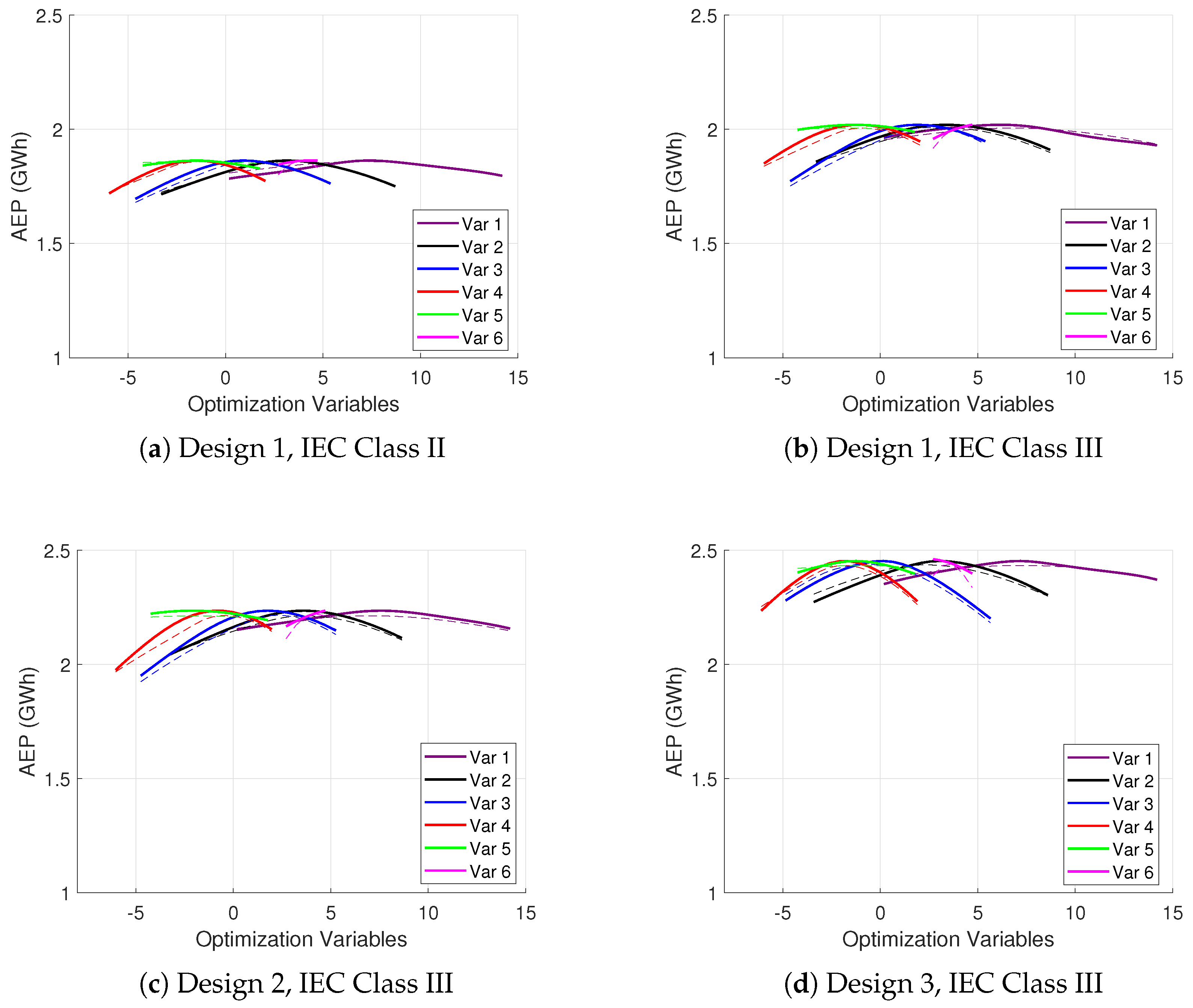
To verify the final accuracy of the SM, a validation test was performed for the three design configurations by comparing its predictions to results generated using the aerodynamic simulations performed with the AeroDyn.v15 module.

The validation was conducted for all four SMs defined in the case study, i.e., the $AE{P}_{12}$ function for a rotor with the same radius as the reference blade under Class II and Class III winds, and rotors with a 5% and 10% increase in radius for Class III wind. The test involved fixing 5 of the 6 design parameters and varying the remaining parameter from its lower to upper bounds. For each combination (which generally falls outside the training grid point set), $AE{P}_{12}$ was computed first through the SM and then with the AeroDyn.v15 module. The results of the tests are shown in Figure 5a (Design 1-IEC Class II), Figure 5b (Design 1-IEC Class III), Figure 5c (Design 2-IEC Class III), and Figure 5d (Design 3-IEC Class III).

The validation results for the SM demonstrated consistent accuracy in predicting the cost function values when compared to those obtained through AeroDyn.v15 simulations.

For the Design 1 (R) configuration under IEC Class II conditions, the SM achieved a close match with the AeroDyn-generated $AE{P}_{12}$ values, with a discrepancy of less than 2%, confirming the reliability of the model in capturing the essential aerodynamic characteristics under higher wind speeds. Similarly, for the IEC Class III conditions, the SM maintained the same level of accuracy, with deviations from the aerodynamic simulation results also being under 2% for all rotor radius cases. A minimal discrepancy was observed for the case of Design 2 when varying the twist angle of the high-midspan control point.

The lower accuracy observed in the SM for the chord variable is attributed to the current definition of the objective function, which focuses on maximizing the $AE{P}_{12}$. $AE{P}_{12}$ is predominantly influenced by the twist distribution, as it directly impacts the aerodynamic efficiency of the blade profile, while the chord distribution has a weaker correlation with this specific objective. By including additional objectives such as weight minimization, which is more directly influenced by the chord distribution, the SM is expected to achieve better performance in managing the chord variable.

4.2. Stochastic Convergence Test

To verify the consistency and robustness of the optimization framework, a test was conducted, performing 80 independent optimization runs with the same setup but randomly varying the initial conditions for the six design variables. The variables were perturbed within their allowable ranges. Statistical metrics, including the mean, standard deviation (std), range, and coefficient of variation (CV), were computed for each parameter. The CV was calculated as $\mathrm{std}/(\mathrm{ub}-\mathrm{lb})$, representing variability relative to the allowable range of each variable.

Table 1. Statistical results of the random test analysis for optimized twist ($\theta$) and chord (c) distributions.

Parameter	Mean	Std	Range	CV
${\theta }_1$	6.98	0.14	0.29	0.01
${\theta }_2$	2.88	0.11	0.22	0.01
${\theta }_3$	0.70	0.26	0.52	0.03
${\theta }_4$	−1.76	0.15	0.30	0.02
${\theta }_5$	−1.34	0.03	0.07	0.006
c	3.94	0.24	0.48	0.24

summarizes the results. The results indicate that the optimization framework consistently converges to the same solution, with low CV for all variables relative to their respective design spaces.

5. Results

This section presents the outcomes of the optimization process for the aerodynamic design of the wind turbine blade, verified through the computation of the complete wind turbine power curve and blade loads using OpenFAST.v3.5.1, an aero-servo-elastic simulation library for wind turbine simulation [34]. The results are evaluated for different rotor configurations, i.e., variations in the blade radius and geometrical parameters such as twist and chord.

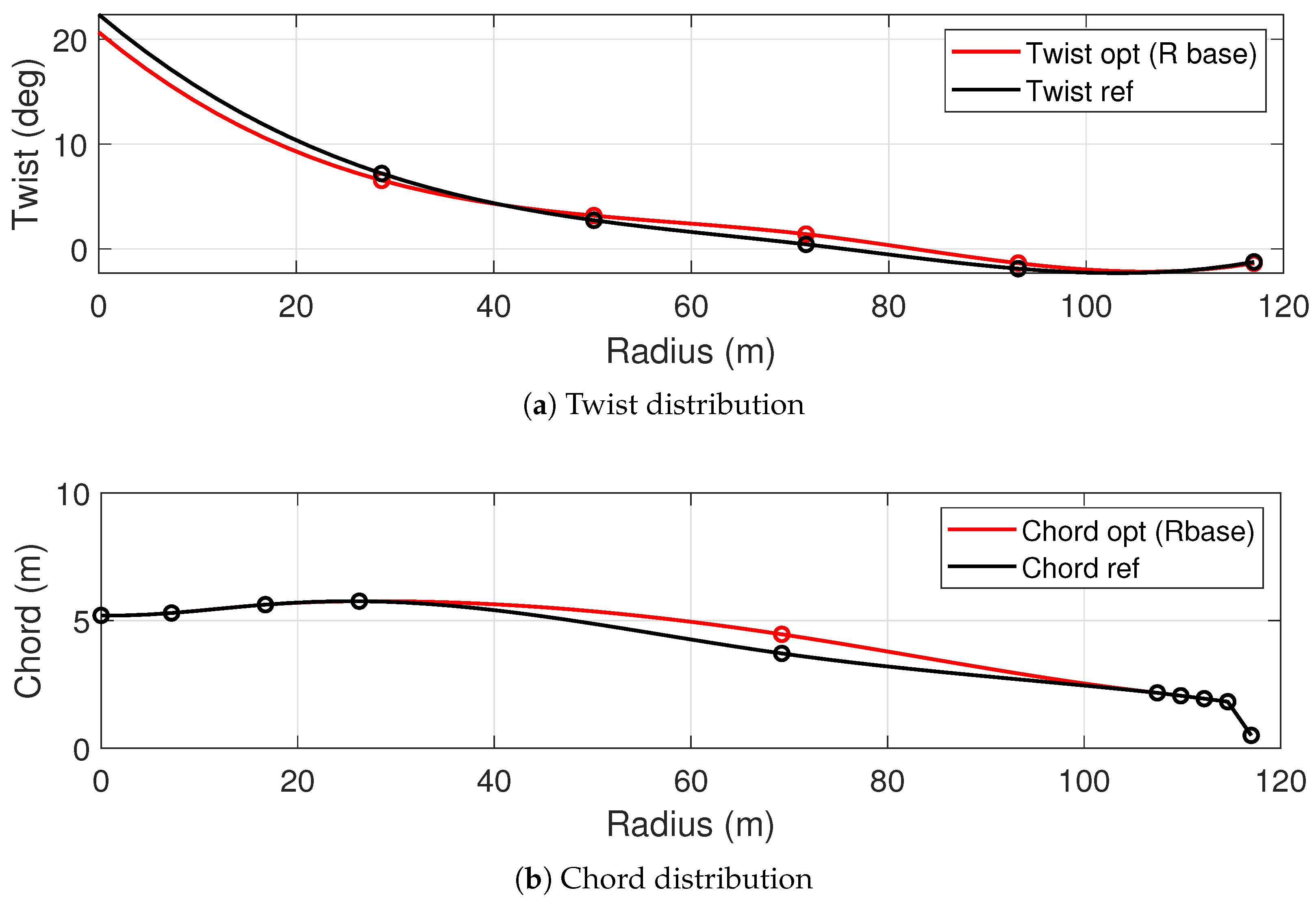
Figure 6 shows the optimization process for Design 1—a rotor with the reference turbine’s base radius of 121 m, optimized for an IEC Class II wind. This test verifies whether the optimization framework can correctly match the performance of the RWT design of the IEA 15 MW, which was optimized for the same wind class. The optimized configuration, characterized by the twist and chord shown in Figure 6a and Figure 6b, respectively, leads to a slight improvement in aerodynamic performance. The $AE{P}_{12}$ for the optimized turbine is 2.021 GWh, with a maximum power coefficient ($C_p$) of 0.489, compared to the reference turbine’s $AE{P}_{12}$ of 2.015 GWh and $C_p$ of 0.487. Although the increase in $AE{P}_{12}$ and $C_p$ is marginal and within the 2% accuracy expected from the SM used in the optimization, these results demonstrate the effectiveness of the GA in fine-tuning blade geometry for enhanced performance.

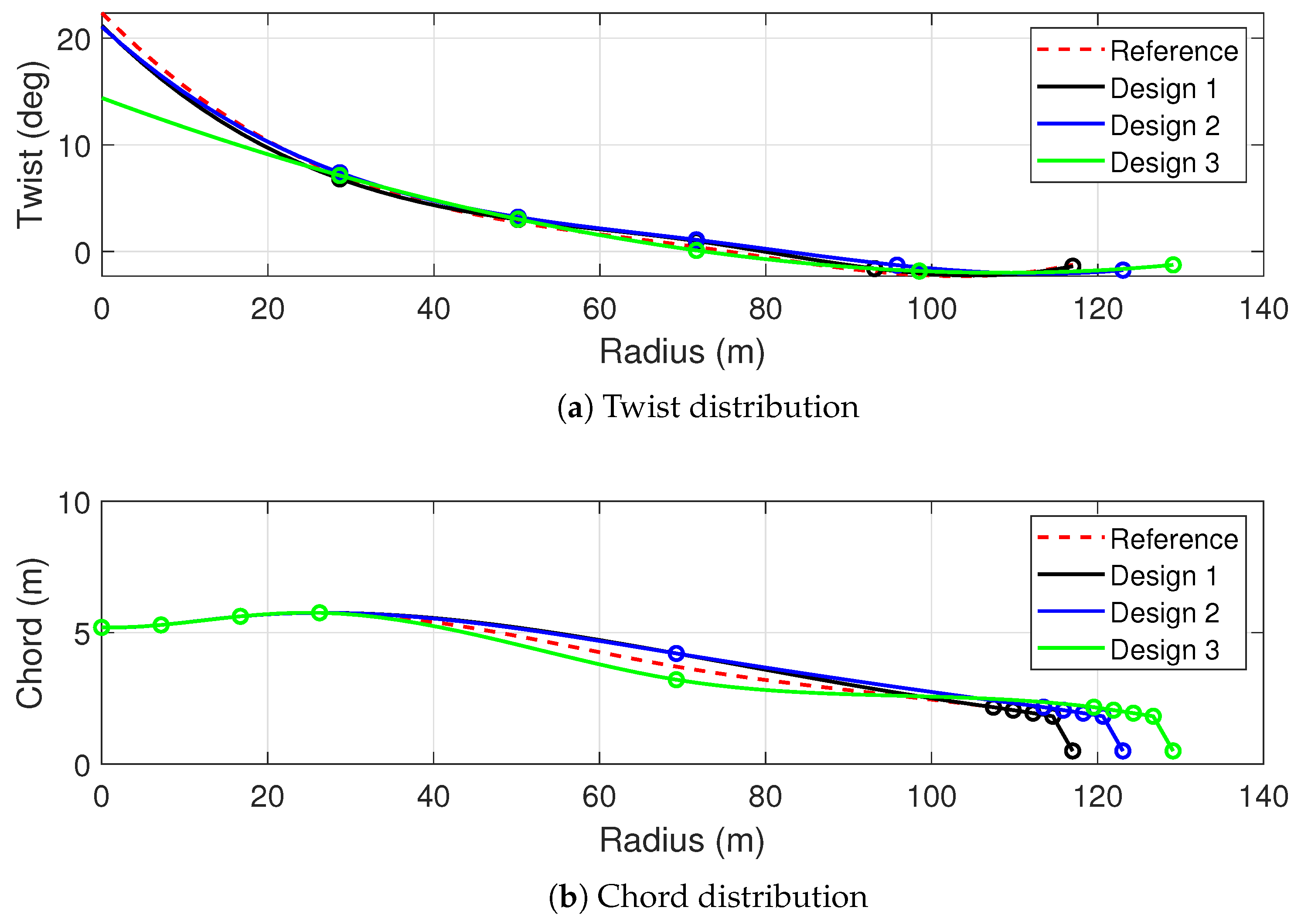
The optimization process was applied to define optimal blades for IEC Class III wind conditions, with two additional configurations featuring increased rotor sizes: Design 2 (+5%R) and Design 3 (+10%R). The size of these augmentations was such that we could confidently retain the original blade profiles and internal architecture, ensuring that the modifications resulted in minimal structural changes. 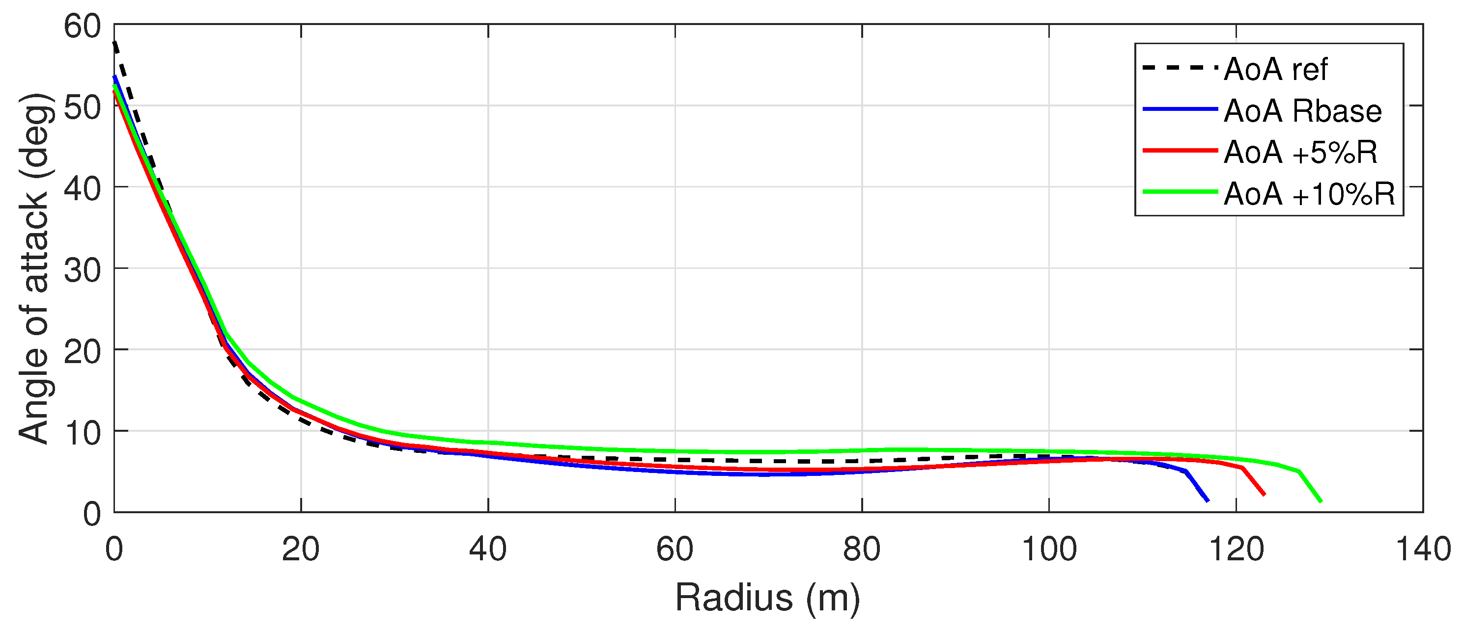The results of these optimizations are shown in Figure 7. The results show that with increasing blade size, the optimal twist and chord distributions for Designs 1 and 2 are similar, while a different trend is followed for the case with a 10% radius increase. To further investigate the results in terms of aerodynamic behavior of the blades, Figure 8 illustrates the radial distribution of the angle of attack (AoA) for the different test cases. Across all configurations, the AoA exhibits the typical trend due to changing relative velocities along the span. Differences are noticeable in the midspan region, where 3D effects are less significant, and the 2D-based BEMT design optimizes the aerodynamic load to achieve the best induction and torque. The aerodynamic load of the blade strip depends on the lift, drag, induction, and peripheral velocity, as well as the chord length. Therefore, we observe that Designs 1 and 2, which have larger chord lengths in this area, require smaller angles of attack compared to the reference design and Design 3 to achieve the same local aerodynamic load. Additionally, the constraint of maintaining the same TSR for all designs forces Designs 2 and 3 to operate at lower rotational velocities, requiring larger angles of attack for Design 2 compared to Design 1, and for Design 3 compared to all others.

The power curves for the reference and optimized configurations were obtained by running OpenFAST simulations of the rigid rotor, assuming a constant tip speed ratio in Region 2 (variable speed generator) and constant power in Region 3. As expected, increasing the rotor size reduces the nominal power density and also reduces the wind speed at which the rotor reaches nominal power. Therefore, Region 3 is defined by assuming that the pitch control is activated to limit the maximum power to 15 MW. 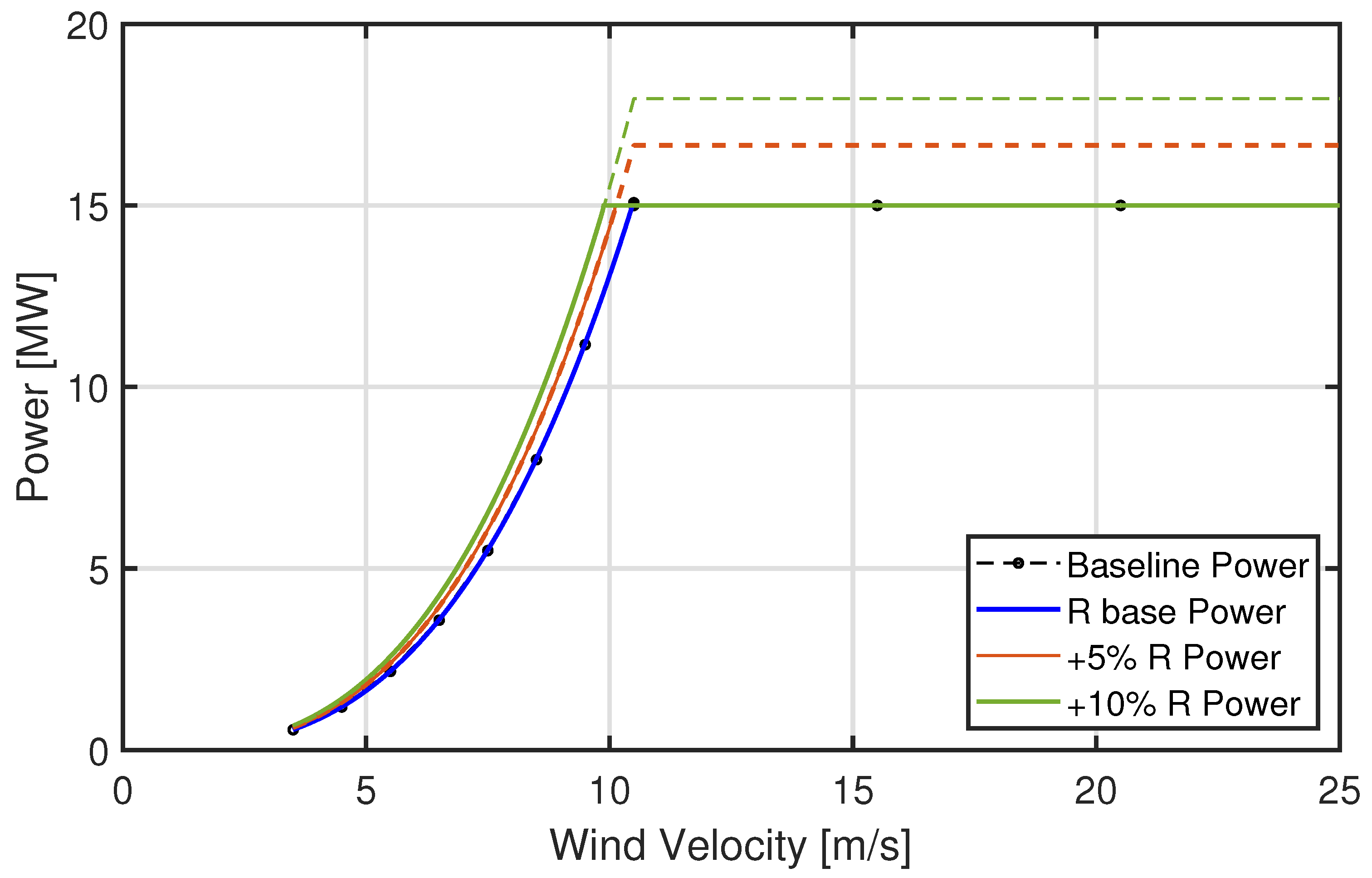Figure 9 shows the power output as a function of wind speed for four different rotor configurations: the reference turbine is shown as a dashed black line; Design 1’s power curve is a solid blue line; Design 2 (+5% R) is a solid orange line; and Design 3 (+10% R) is a solid green line. These curves illustrate the performance of the turbine across a range of wind speeds, from cut-in to rated and cut-out speeds.

The OpenFAST.v3.5.1 simulations were conducted with a steady wind defined by the same power law exponent defined previously. The simulation ran for 300 s, and the rotor power value was averaged over the last 100 s. As shown in Figure 9, increasing the rotor radius results in an upward shift in the power curve, especially in the rated region, where the larger blades capture more energy.

Table 2. Comparison of aerodynamic performance coefficients ($C_p$) and annual energy production ($AE{P}_{12}$) for the reference and optimized rotor design. Results show incremental improvements in $AE{P}_{12}$ with increasing rotor size, despite minor variations in $C_p$.

Design	${\mathit{C}}_{\mathit{p}}$	${\mathit{AEP}}_{\mathbf{12}}$ (GWh)
Reference	0.487	2.015
Design 1	0.489	2.021
Design 2	0.488	2.230
Design 3	0.486	2.430

provides details on the target performance in terms of total energy production across the entire wind speed range.

Table 3. Comparison of Annual Energy Production ($AE{P}_{12}$) and Capacity Factor (CF) for the different rotor designs and for IEC Wind Classes 2, 3, and 4.

Design	IEC Class II ${\mathbf{AEP}}_{12}$ (GWh)	IEC Class II CF	$\mathbf{\Delta }\%$
Reference	67.114	0.511	-
Design 1	67.211	0.512	0.1
Design 2	69.831	0.531	4.1
Design 3	71.826	0.547	7.0
	IEC Class III ${\mathbf{AEP}}_{\mathbf{12}}$ (GWh)	IEC Class III CF	$\mathrm{\Delta }\%$
Reference	56.591	0.431	-
Design 1	56.691	0.431	0.2
Design 2	59.405	0.452	5.0
Design 3	61.494	0.468	8.7
	IEC Class IV ${\mathbf{AEP}}_{\mathbf{12}}$ (GWh)	IEC Class IV CF	$\mathrm{\Delta }\%$
Reference	50.672	0.386	-
Design 1	50.771	0.386	0.2
Design 2	53.478	0.407	5.5
Design 3	55.576	0.423	9.7

summarizes the $AE{P}_{12}$, capacity factor (CF), and percentage increase in $AE{P}_{12}$ ($\mathrm{\Delta }\%$) with respect to the value obtained with the same wind class using the reference IEA 15 MW design. As shown, the $AE{P}_{12}$ increases with larger rotor sizes, leading to an increase in CF, highlighting the aerodynamic gains from the optimized blade geometries.

The computation was performed for three different IEC wind classes: II, III, and IV. The optimized configurations consistently yielded higher $AE{P}_{12}$ values, with the percentage increase reaching up to 9.7% for Class IV conditions, corresponding to a 10% increase in rotor size. These results highlight the effectiveness of the proposed design optimizations in enhancing energy capture, particularly in lower wind classes.

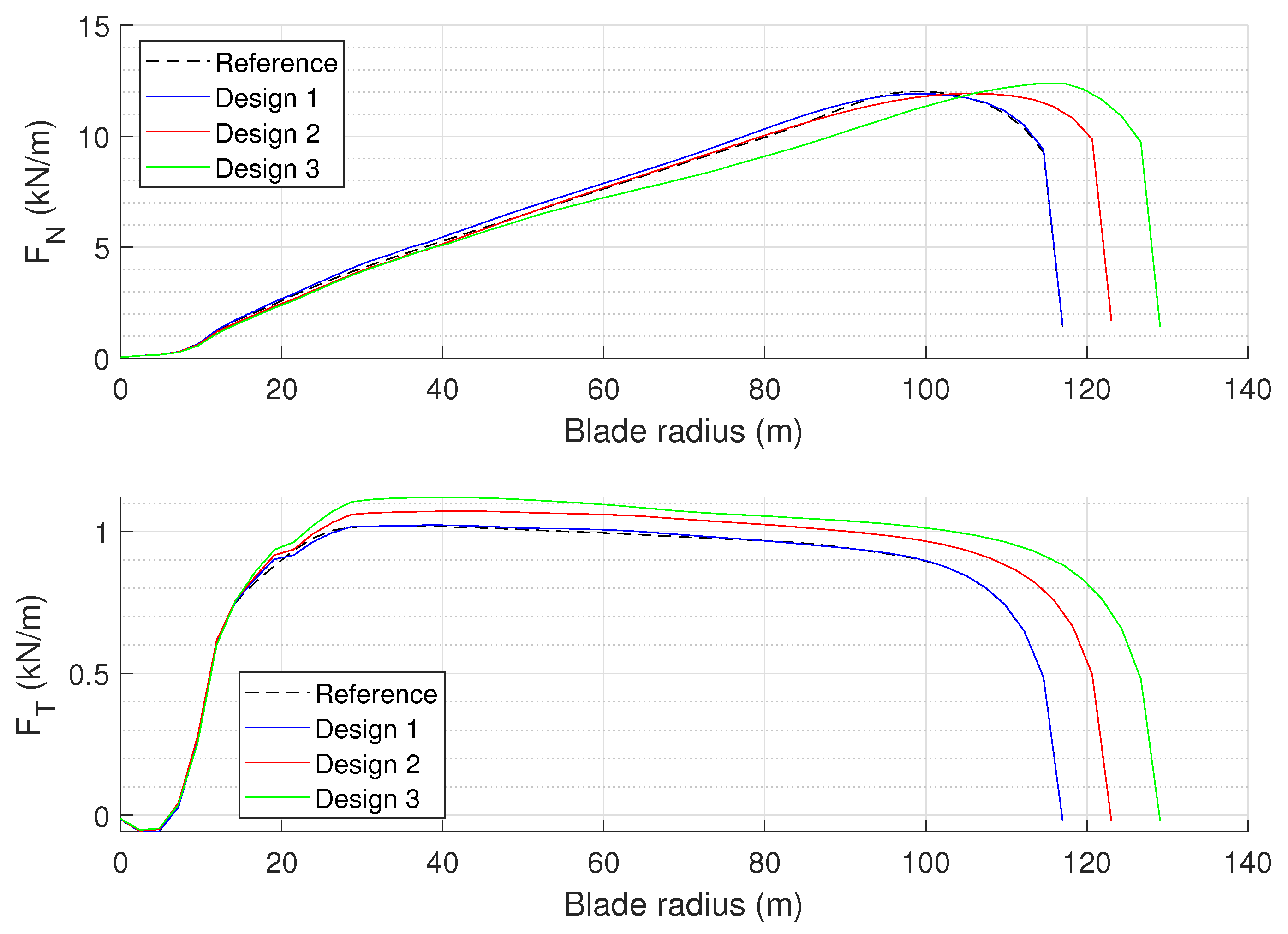
The impact of the optimized blade designs in terms of blade loads was also verified. The aerodynamic forces (shown in Figure 10) acting on the wind turbine blade have a direct impact on the flap-wise and edge-wise bending moments at the root, which are critical parameters in structural design and fatigue assessment. The normal and tangential force distributions along the blade span were analyzed at a steady wind speed of 10.5 m/s (see

Table 4. Normal and tangential force per unit length for different blade designs. $F_n$ represents the normal force, while $F_t$ represents the tangential force.

Design	${\mathit{F}}_{\mathit{n}}$ (kN/m)	${\mathit{F}}_{\mathit{t}}$ (kN/m)
Reference	12.0	1.10
Design 1	12.0	1.10
Design 2	12.0	1.06
Design 3	12.4	1.10

), alongside the increase in integral root bending moments due to variations in blade length.

The normal force, which primarily drives flap-wise bending moments, varies along the blade span and reaches a peak value of 12.0 kN/m near the tip for the reference design. In the optimized configurations, particularly Design 2 and Design 3, the normal force distribution exhibits a slight increase (reaching 12.4 kN/m) in the outer span. The tangential force, which contributes to torque generation and influences edge-wise bending moments, remains relatively stable across different blade designs.

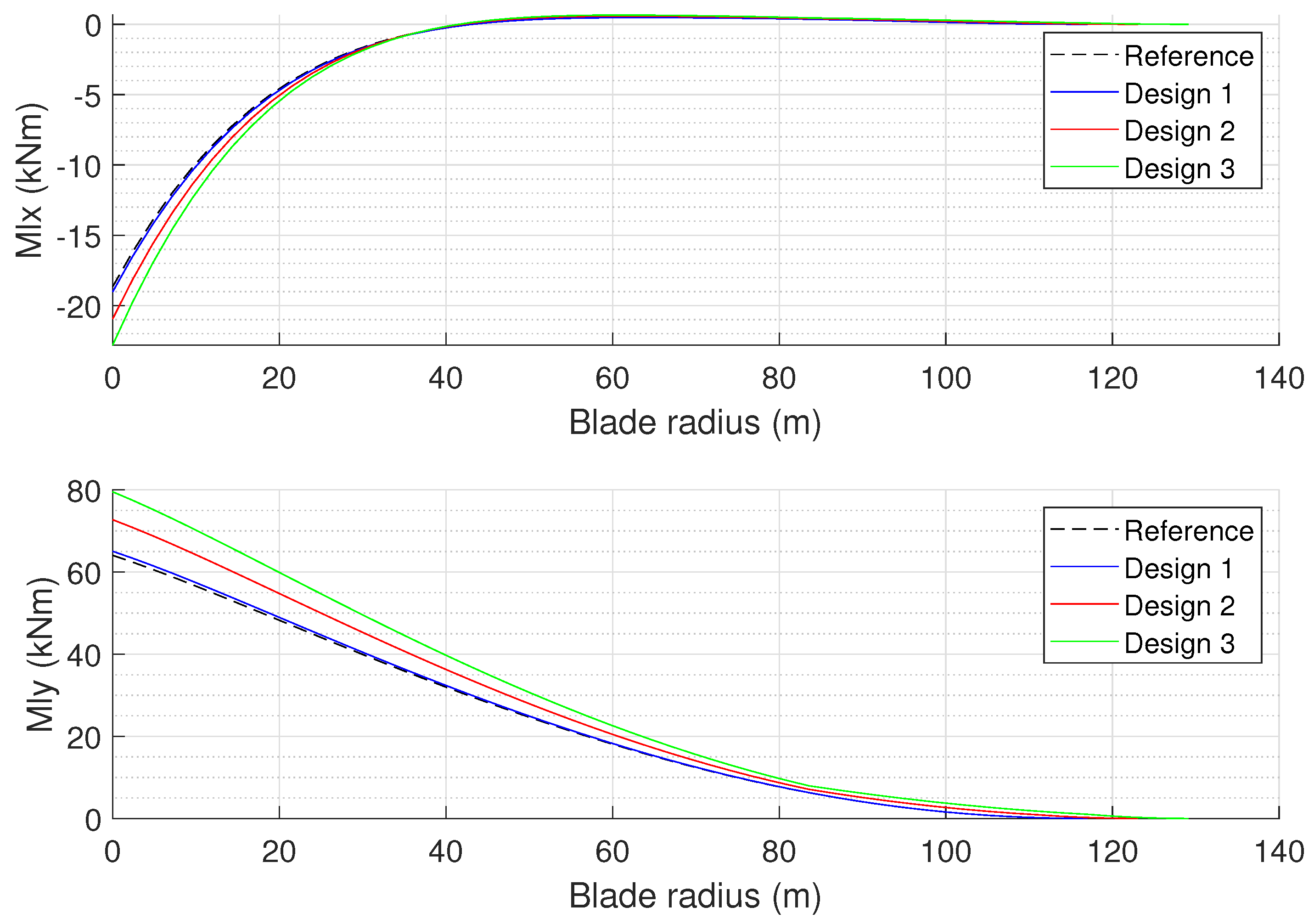
As a result, the root bending moments exhibit an increase for Design 2 and 3 with respect to the baseline blade, as shown in Figure 11. The flap-wise moment increases by 13.5% and 24.1% for Designs 2 and 3, respectively, while the edge-wise moment, driven by the gravity and inertial effects, increases by 12.3% in Design 2 and 22.2% in Design 3. These trends, summarized in

Table 5. Percentage increase in flap-wise and edge-wise bending moments at the blade root for different blade designs relative to the reference turbine (R).

Design	Edge-Wise ($\mathbf{\Delta }\%$)	Flap-Wise ($\mathbf{\Delta }\%$)
Reference	-	-
Design 1	1.5	1.9
Design 2	13.5	12.3
Design 3	24.1	22.2

, indicate that while aerodynamic optimization improves energy capture, the structural implications should be carefully addressed by increasing the root section resistance.

While the increases in aerodynamic forces and structural loads present challenges in terms of fatigue life and material stresses, these effects must be evaluated in the broader context of energy production. The trade-off between increased loads and enhanced power output is a key consideration in the aerodynamic optimization process. Although a larger rotor experiences higher root bending moments, it is able to capture more energy at lower wind speeds, which is the main target of a wind turbine design for Mediterranean Sea applications.

6. Conclusions

This study presents an SM-based optimization framework for the aerodynamic design of wind turbine blades, applicable to various wind and turbine types and classes. Its effectiveness is demonstrated through a case study focused on the challenging offshore and low-speed wind conditions found at Mediterranean Sea sites. The SM, employing SRBF, was developed to reduce the computational cost associated with high-fidelity simulations while maintaining predictive accuracy. Validation of the SM against aerodynamic simulations using AeroDyn.v15 demonstrated the high degree of accuracy of the surrogate model training, with discrepancies of less than 2%, confirming its reliability for aerodynamic performance prediction.

The optimization process, driven by a GA, focused on the twist and chord distributions along the blade span to maximize the AEP in Region 2 of the power curve. The optimized blade configuration with a base radius of 121 m presented a slight improvement in $AE{P}_{12}$, from 2.015 GWh to 2.021 GWh, and a slight increase in the $C_p$, from 0.487 to 0.489, compared to a Reference Wind Turbine (RWT) design of the same scale reported in the literature. Significant increases were realized with augmented rotor sizes, where a 5% increase in blade radius led to an $AE{P}_{12}$ of 2.23 GWh, and a 10% increase achieved 2.43 GWh. These results demonstrate the effectiveness of the optimization process in producing an efficient turbine blade design for low wind speeds.

Future work will focus on enhancing the surrogate modeling framework by incorporating high-fidelity CFD simulations. This enhancement will allow the framework to capture complex aerodynamic phenomena with greater accuracy. Additionally, these developments will facilitate the framework’s extension to multi-objective optimization, addressing trade-offs between structural integrity, cost minimization, and aerodynamic performance. Future studies may also explore substituting the BEMT-based full-order model with more complex simulation models, accounting for a broader range of operational aspects specific to floating offshore wind turbines. Such advancements will enable the introduction of additional objectives, such as weight, lifespan, and constraints related to structural integrity and fatigue resistance, further extending the applicability and impact of this optimization framework.

References

- Global Wind Energy Council. Global Offshore Wind Report 2020; GWEC: Brussels, Belgium, 2020; Volume 19, pp. 10–12. [Google Scholar]
- WindEurope. Wind Energy in Europe: 2021 Statistics and the Outlook for 2022–2026; Technical Report; Wind Europe Report: Brussels, Belgium, 2022. [Google Scholar]
- Heidari, S. Economic Modelling of Floating Offshore Wind Power: Calculation of Levelized Cost of Energy. Ph.D. Thesis, Industrial Economics and Organisation, Mälardalen University, Västerås, Sweden, 2017; 82p. [Google Scholar]
- Barnabei, V.F.; Ancora, T.C.M.; Conti, M.; Castorrini, A.; Delibra, G.; Corsini, A.; Rispoli, F. A Multi-Objective Optimization Framework for Offshore Wind Farm Design in Deep Water Seas. J. Fluids Eng. 2024, 147, 031105. [Google Scholar] [CrossRef]
- Ashuri, T.; Zaaijer, M.; Martins, J.; van Bussel, G.; van Kuik, G. Multidisciplinary design optimization of offshore wind turbines for minimum levelized cost of energy. Renew. Energy 2014, 68, 893–905. [Google Scholar] [CrossRef]
- Fuglsang, P.; Madsen, H.A. Optimization method for wind turbine rotors. J. Wind Eng. Ind. Aerodyn. 1999, 80, 191–206. [Google Scholar] [CrossRef]
- Maki, K.; Sbragio, R.; Vlahopoulos, N. System design of a wind turbine using a multi-level optimization approach. Renew. Energy 2012, 43, 101–110. [Google Scholar] [CrossRef]
- Andrew Ning, S.; Damiani, R.; Moriarty, P.J. Objectives and constraints for wind turbine optimization. J. Sol. Energy Eng. 2014, 136, 041010. [Google Scholar] [CrossRef]
- Bottasso, C.L.; Campagnolo, F.; Croce, A. Multi-disciplinary constrained optimization of wind turbines. Multibody Syst. Dyn. 2012, 27, 21–53. [Google Scholar] [CrossRef]
- Bottasso, C.L.; Bortolotti, P.; Croce, A.; Gualdoni, F. Integrated aero-structural optimization of wind turbines. Multibody Syst. Dyn. 2016, 38, 317–344. [Google Scholar] [CrossRef]
- Bortolotti, P.; Bottasso, C.L.; Croce, A. Combined preliminary–detailed design of wind turbines. Wind Energy Sci. 2016, 1, 71–88. [Google Scholar] [CrossRef]
- Jonkman, J.; Butterfield, S.; Musial, W.; Scott, G. Definition of a 5-MW Reference Wind Turbine for Offshore System Development; National Renewable Energy Laboratory: Golden, CO, USA, 2009. [Google Scholar]
- Bak, C.; Zahle, F.; Bitsche, R.; Kim, T.; Yde, A.; Henriksen, L.C.; Hansen, M.H.; Blasques, J.P.A.A.; Gaunaa, M.; Natarajan, A. The DTU 10-MW reference wind turbine. In Proceedings of the Danish Wind Power Research 2013, Fredericia, Denmark, 27–28 May 2013. [Google Scholar]
- Gaertner, E. Definition of the IEA 15-Megawatt Offshore Reference Wind; National Renewable Energy Laboratory: Golden, CO, USA, 2020. [Google Scholar]
- Forrester, A.I.; Sóbester, A.; Keane, A.J. Multi-fidelity optimization via surrogate modelling. Proc. R. Soc. A Math. Phys. Eng. Sci. 2007, 463, 3251–3269. [Google Scholar] [CrossRef]
- Fernández-Godino, M.G. Review of multi-fidelity models. arXiv 2016, arXiv:1609.07196. [Google Scholar]
- Pellegrini, R.; Wackers, J.; Broglia, R.; Serani, A.; Visonneau, M.; Diez, M. A multi-fidelity active learning method for global design optimization problems with noisy evaluations. Eng. Comput. 2023, 39, 3183–3206. [Google Scholar] [CrossRef]
- Wackers, J.; Visonneau, M.; Serani, A.; Pellegrini, R.; Broglia, R.; Diez, M. Multi-fidelity machine learning from adaptive-and multi-grid RANS simulations. In Proceedings of the 33rd Symposium on Naval Hydrodynamics, Osaka, Japan, 18–23 October 2020. [Google Scholar]
- Forrester, A.; Sobester, A.; Keane, A. University of Southamptom, UK Engineering Design via Surrogate Modelling: A Practical Guide; John Wiley & Sons Ltd., The Atrium: Chichester, UK, 2008. [Google Scholar]
- Han, Z.H.; Zimmermann, R.; Görtz, S. Alternative cokriging method for variable-fidelity surrogate modeling. AIAA J. 2012, 50, 1205–1210. [Google Scholar] [CrossRef]
- Tamaki, H.; Kita, H.; Kobayashi, S. Multi-objective optimization by genetic algorithms: A review. In Proceedings of the IEEE International Conference on Evolutionary Computation, Nagoya, Japan, 20–22 May 1996; pp. 517–522. [Google Scholar] [CrossRef]
- Konak, A.; Coit, D.W.; Smith, A.E. Multi-objective optimization using genetic algorithms: A tutorial. Reliab. Eng. Syst. Saf. 2006, 91, 992–1007. [Google Scholar] [CrossRef]
- Cardamone, R.; Broglia, R.; Papi, F.; Rispoli, F.; Corsini, A.; Bianchini, A.; Castorrini, A. Aerodynamic design of wind turbine blades using multi-fidelity analysis and surrogate models. In Proceedings of the 16th European Conference on Turbomachinery Fluid dynamics & Thermodynamics (ETC), Hannover, Germany, 24–28 March 2025. [Google Scholar]
- Jasa, J.; Bortolotti, P.; Zalkind, D.; Barter, G. Effectively using multifidelity optimization for wind turbine design. Wind Energy Sci. 2022, 7, 991–1006. [Google Scholar] [CrossRef]
- Volpi, S.; Diez, M.; Stern, F. Multidisciplinary design optimization of a 3D composite hydrofoil via variable accuracy architecture. In Proceedings of the 2018 Multidisciplinary Analysis and Optimization Conference, Atlanta, Georgia, 25–29 June 2018; p. 4173. [Google Scholar]
- Castorrini, A.; Ortolani, A.; Campobasso, M.S. Assessing the progression of wind turbine energy yield losses due to blade erosion by resolving damage geometries from lab tests and field observations. Renew. Energy 2023, 218, 119256. [Google Scholar] [CrossRef]
- Lux, O.; Lemmerz, C.; Weiler, F.; Marksteiner, U.; Witschas, B.; Rahm, S.; Geiß, A.; Reitebuch, O. Intercomparison of wind observations from the European Space Agency’s Aeolus satellite mission and the ALADIN Airborne Demonstrator. Atmos. Meas. Tech. 2020, 13, 2075–2097. [Google Scholar] [CrossRef]
- Dee, D.P.; Uppala, S.M.; Simmons, A.J.; Berrisford, P.; Poli, P.; Kobayashi, S.; Andrae, U.; Balmaseda, M.; Balsamo, G.; Bauer, d.P.; et al. The ERA-Interim reanalysis: Configuration and performance of the data assimilation system. Q. J. R. Meteorol. Soc. 2011, 137, 553–597. [Google Scholar] [CrossRef]
- NOSTRUM—Optimizing Floating Offshore Wind Turbines for Use in the Mediterranean Sea. Available online: https://nostrum-project.it (accessed on 17 January 2025).
- Hersbach, H.; Bell, B.; Berrisford, P.; Biavati, G.; Horányi, A.; Muñoz Sabater, J.; Nicolas, J.; Peubey, C.; Radu, R.; Rozum, I.; et al. ERA5 hourly data on single levels from 1979 to present. Copernic. Clim. Chang. Serv. (c3s) Clim. Data Store (cds) 2018. [Google Scholar] [CrossRef]
- IEC 61400-3-1; Wind Energy Generation Systems-Part 3-1: Design Requirements for Fixed Offshore Wind Turbines. International Electrotechnical Commission: Geneva, Switzerland, 2019.
- Hopstad, A.L.H.; Argyriadis, K.; Manjock, A.; Goldsmith, J.; Ronold, K.O. DNV GL standard for floating wind turbines. In Proceedings of the International Conference on Offshore Mechanics and Arctic Engineering, Madrid, Spain, 17–22 June 2018; American Society of Mechanical Engineers: New York, NY, USA, 2018; Volume 51975, p. V001T01A020. [Google Scholar]
- Moriarty, P.J.; Hansen, A.C. AeroDyn Theory Manual; National Renewable Energy Laboratory: Golden, CO, USA, 2005. [Google Scholar] [CrossRef]
- Jonkman, J.; Sprague, M. OpenFAST: An Aeroelastic Computer-Aided Engineering Tool for Horizontal Axis Wind Turbines. 2022. Available online: https://www.nrel.gov/wind/nwtc/openfast.html (accessed on 15 September 2024).
Figure 1.
Design space control points (black markers), spline interpolation (black line), and reference blade values (red dashed line) for the twist and chord distributions along the blade span.
Figure 2.
Sensitivity analysis of the parameter in the k- SST turbulence model for the FFA-W3-301 (top) and FFA-W3-330 (bottom) airfoils. The aerodynamic coefficients are computed using for FFA-W3-301 and for FFA-W3-330, in agreement with the reference IEA 15MW dataset.
Figure 3.
Comparison of lift and drag coefficients for the FFA−W3−301 (top) and FFA−W3−330 (bottom) airfoils. CFD results are shown for three Reynolds numbers (, , and ) and compared against reference IEA data (red dots).
Figure 4.
Thickness distribution along the blade span for the three test cases: Design 1 (R), Design 2 (+5%R), and Design 3 (+10%R).
Figure 5.
Validation of the surrogate model for different blade designs and IEC wind classes. Each subfigure compares the surrogate model predictions (continuous lines) with the FOM computations performed using AeroDyn.v15 (dashed lines). Subfigures (a,b) refer to Design 1 under IEC Class II and Class III conditions, respectively; subfigures (c,d) show the results for Design 2 and Design 3, both evaluated under IEC Class III conditions.
Figure 6.
Optimized twist and chord distributions for Design 1 (R). The red curves represent the optimized distributions obtained from the GA, while the black curves correspond to the reference turbine’s twist and chord distributions.
Figure 7.
Optimized twist and chord distribution for Design 2 wind turbine. The curves represent the optimized distributions obtained from the GA.
Figure 8.
Angle of attack as a function of radius for the four tests. Reference configuration (dashed black line); Design 1 (solid blue line), Design 2 (solid red line), Design 3 (solid green line).
Figure 9.
Rotor power curves as a function of wind speed for the four tests. Reference configuration (dashed black line); Design 1 (solid blue line), Design 2 (solid orange line), Design 3 (solid green line).
Figure 10.
Spanwise distribution of normal (top) and tangential (bottom) aerodynamic forces for the reference and optimized blade designs at 10.5 m/s.
Figure 11.
Spanwise distribution of edgewise (top) and flapwise (bottom) bending moments for the reference and optimized blade designs at 10.5 m/s.