An Open Test Case for High-Speed Low-Pressure Turbines: The SPLEEN C1 Cascade ^†

Abstract

Aviation accounts for a significant share of global CO₂ emissions, necessitating efficient propulsion technologies to achieve net-zero emissions by 2050. Geared turbofan architectures offer a promising solution by enabling higher bypass ratios and improved fuel efficiency. However, geared turbofans introduce significant aerodynamic and structural challenges, particularly in the low-pressure turbine. Current understanding of high-speed low-pressure turbine behavior under engine-representative conditions is limited, especially regarding unsteady wake interactions, secondary flows, and compressibility effects. To address these gaps, this work presents a novel test case of high-speed low-pressure turbines, the SPLEEN C1. The test case and experimental methodology are depicted. The study includes the commissioning and characterization of a transonic low-density linear cascade capable of testing quasi-3D flows. The rig’s operational stability, periodicity, and inlet flow characterization are assessed in terms of loss and turbulence quantities to ensure an accurate representation of engine conditions. These findings provide a validated experimental platform for studying complex flow interactions in high-speed low-pressure turbines, supporting future turbine design and efficiency advancements.

1. Introduction

Aviation accounts for 3% of global ${\mathrm{CO}}_2$ emissions, and 4% in Europe [1,2], with the Flightpath2050 initiative targeting net-zero emissions by 2050. This requires reducing ${\mathrm{CO}}_2$, NOx, and noise by 75%, 90%, and 65%, respectively, compared to 2000 levels. Despite efficiency improvements that have cut ${\mathrm{CO}}_2$ emissions by over 50% since 1990 [3], growth in air traffic risks offsetting these gains, with emissions projected to hit 2000 Mt by 2050 without further action. Gas turbines remain essential for cutting emissions, particularly on short- and medium-haul flights, which are forecast to account for 55% of ${\mathrm{CO}}_2$ emissions while representing over 90% of flights by 2050 (https://www.clean-aviation.eu/media/publications/technology-evaluator-first-global-assessment-2020-technical-report, accessed on 6 January 2025).

Increasing turbofan propulsive efficiency, particularly through higher bypass ratios (BPR), is a key approach to lowering specific fuel consumption (SFC) [4]. However, further increases in BPR are limited by fan size, nacelle drag, and challenges around integration with the airframe [5,6,7]. Geared turbofan (GTF) architectures address these issues by decoupling the fan and low-pressure turbine (LPT) speeds, enabling larger fans and higher bypass ratio without compromising performance [4].

Geared turbofans (GTFs) achieve significant reductions in specific fuel consumption (SFC), especially at bypass ratios (BPR) above 10. The low-pressure turbine in GTFs operates at higher peripheral speeds, allowing lower stage loading and flow coefficients, which leads to fewer stages and improved efficiency [8]. However, these conditions pose aerodynamic and structural challenges such as compressibility effects on losses and boundary layer behavior [9]. At the aerodynamic level, the turbine operates at transonic Mach numbers exceeding 0.80 at the outlet. The faster spool speed introduces greater mechanical loads, necessitating design adaptations [10,11]. Torre et al. [12] demonstrated the changes in operating points in a full-scale intermediate-pressure turbine for geared applications compared to direct-drive turbofans.

Traditionally, research efforts aimed at optimizing the performance of (ultra-) high-lift blade designs [13] have led to extensive characterization of these profiles under both steady and unsteady conditions in fully subsonic low-pressure turbine rigs (${\mathrm{M}}_{out}$ < 0.7). The findings of these studies have been well documented in works such as [14,15,16]. However, as the current focus of industry lies on transonic turbine blades, our understanding of compressible flows over high-speed profiles remains incomplete.

Modern high-speed low-pressure turbine designs require investigating the effect of high Mach numbers and low Reynolds numbers on the interactions of unsteady wakes, secondary, leakage, and purge flows, as well as on the underlying loss mechanisms of high-speed low-pressure turbines [17]. Moreover, at transonic exit Mach numbers, shock–boundary layer interactions occur on the suction-side boundary layer [18].

Malzacher et al. [11] demonstrated the performance enhancement of high-speed low-pressure turbines through two-stage turbine testing at engine-relevant Mach and Reynolds numbers and temperatures. Two blade profiles were tested in a linear cascade at Reynolds numbers of 60,000 and 77,000 with Mach numbers exceeding 0.80. Vera et al. [19,20] conducted linear cascade tests on high-speed turbine profiles at Reynolds numbers starting from 130,000 and Mach numbers between 0.61 and 0.83, examining both steady and unsteady inlet flows. The unsteady wakes were characterized by a bar reduced frequency of 0.47 and 0.35 as the Mach number increased. Steady annular cascade and rotating turbine rig studies by [17] and [21] investigated Mach numbers from 0.50 to 0.90 and Reynolds numbers from 120,000 to 315,000, focusing on the combined effects of unsteady wakes, surface finish, and aerodynamic performance. Boerner and Niehuis [18] analyzed shock–boundary layer interactions in a high-speed linear cascade at Mach ∼0.95 and Reynolds numbers between 100,000 and 200,000, emphasizing shock strength and boundary layer state influences on blade loading and total pressure losses.

Despite these contributions, key aspects remain underexplored. Considering their critical influence on shock–boundary layer interaction and boundary layer transition, further studies are needed on short- to mid-range low-pressure turbines operating at Reynolds numbers between 50,000 and 150,000 [17]. The aerodynamics of low- to mid-lift profiles at transonic Mach numbers (0.90–0.95) also require further investigation [18]. Additionally, experimental data for validating secondary flow models under low Reynolds regimes remain scarce but crucial [22,23]. Real engine flow behavior is strongly influenced by off-design conditions due to shaft speed variations, and also lacks comprehensive experimental data on Reynolds and Mach number effects in high-speed low-pressure turbine conditions [24].

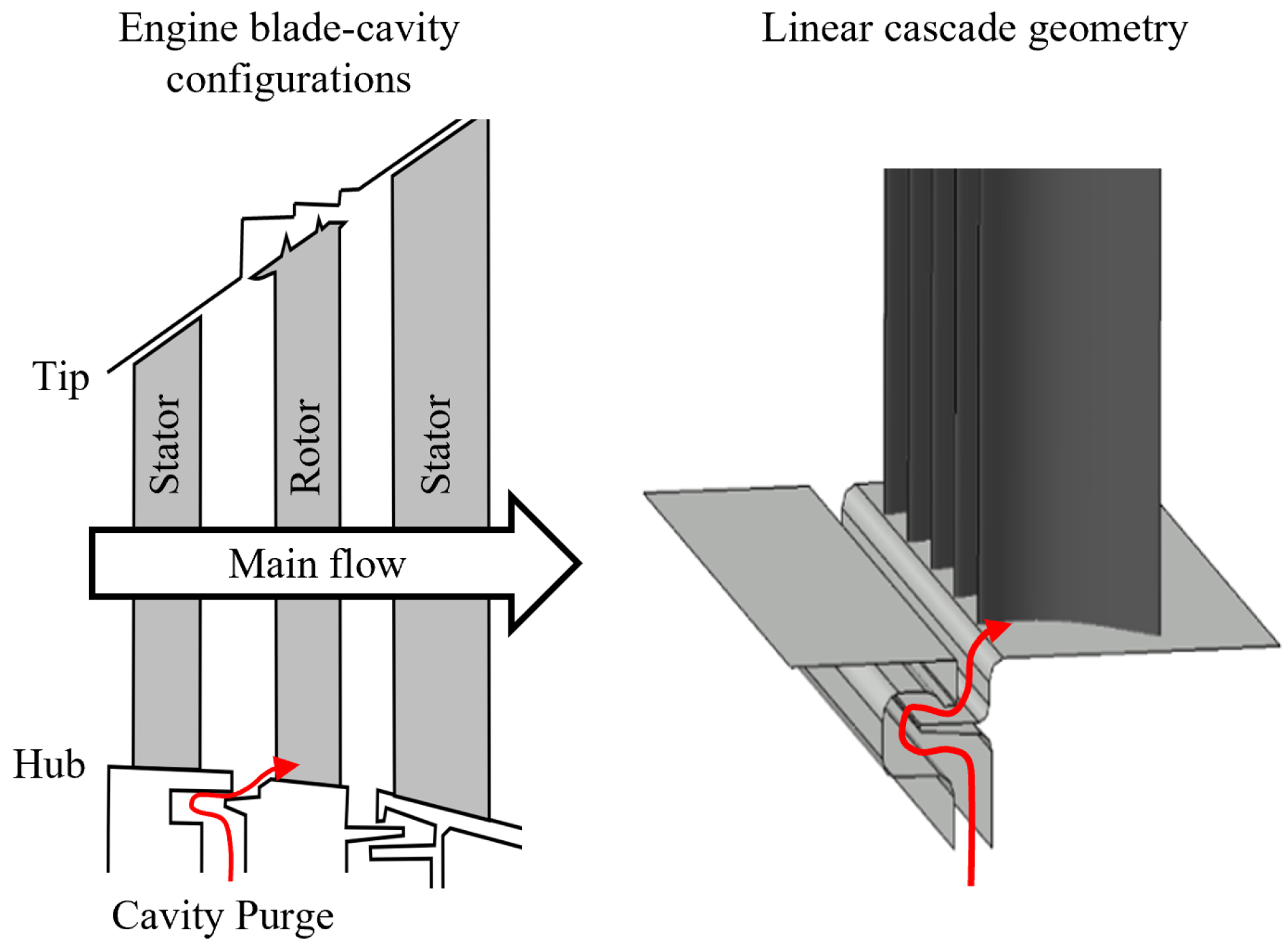
This work introduces the SPLEEN C1, a novel open-access test case for high-speed low-pressure turbines designed to address the gap in high-quality experimental data at engine-relevant conditions. While secondary flows in linear cascades do not fully represent engine environments, they are widely used for secondary flow studies and model correlations [22,23,25,26]. Therefore, linear cascade measurements were chosen to explore secondary flow interactions with turbine blades and to assess the effects of Reynolds and Mach numbers on loss mechanisms and secondary flow characteristics, with high accuracy in boundary condition definition. The experimental rig enables systematic variations in Reynolds numbers between 50,000 and 150,000 and transonic exit Mach numbers from 0.60 to 0.95, while replicating unsteady wake effects and secondary flow features observed in real engine conditions. This setup provides high-fidelity data to improve computational models, focusing on flow phenomena relevant to next-generation geared turbofan engines.

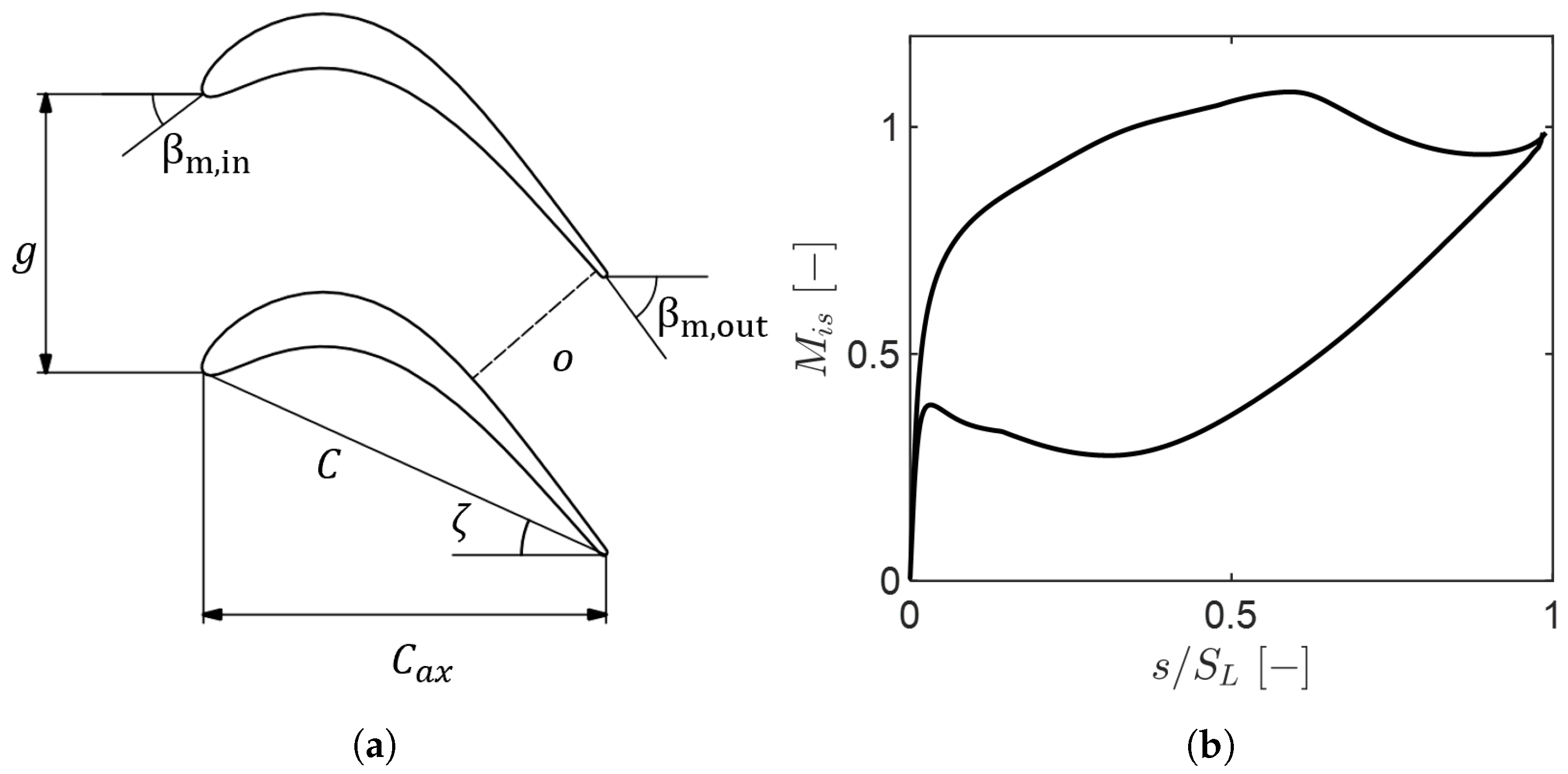
The dataset includes comprehensive measurements of a low-lift profile representative of the hub section of a modern low-pressure turbine blade characterized by a thin laminar open separation bubble. Tests were conducted at Mach numbers between 0.70–0.95 and Reynolds numbers from 65,000–120,000, capturing both 2D blade aerodynamics and endwall flows. These conditions enable a detailed investigation of the effects of Reynolds and Mach numbers under challenging off-design operating conditions, offering valuable data for validating loss models, developing transition models for Reynolds-averaged Navier–Stokes simulations, and validating high-order direct numerical simulations.

This paper describes the test case and experimental methodology, detailing the design of the blade profile and the adaptation of the linear cascade for high-speed 3D aerodynamic testing. Results from the rig commissioning are presented, including flow condition stability, inlet boundary layer characteristics, free stream turbulence intensity, and length scales. The periodicity of the flow field in the cascade is also investigated. The current work updates and expands upon the initial findings published in [27].

The project results, open-access database, and supporting documentation are openly available in Zenodo at https://doi.org/10.5281/zenodo.7264761 (accessed on 6 January 2025).

2. The SPLEEN C1 Test Case

The EU-funded project SPLEEN (Secondary and leakage flow effects in high-sPeed Low-prEssurE turbiNes), led by the von Karman Institute in collaboration with Safran Aircraft Engines (SAE), investigated the combined effects of purge and secondary flows on the performance of high-speed low-pressure turbines. These effects consider unsteady flows resulting from stator–rotor interaction in actual engine conditions. A meridional cut of 1.5 stages of the low-pressure turbine is shown in Figure 1.

The project focused on the influence of stator–rotor hub platform purge flow on secondary flows and rotor aerodynamics near the endwall. The engine-representative geometry in Figure 1 was extruded for testing in a linear cascade arrangement.

2.1. The VKI S-1/C

The linear cascade measurements are conducted in the high-speed low-Reynolds facility S-1/C of the von Karman Institute. This continuous closed-loop wind tunnel is powered by a 615 kW, 13-stage axial flow compressor. A heat exchanger maintains near-ambient flow temperatures, while mass flow is regulated by controlling the compressor speed and a pressure regulation valve. A vacuum pump allows for minimum absolute pressure values as low as 5000 Pa.

A schematic view of the wind tunnel is shown in Figure 2. The cascade test section is mounted in the first elbow of the loop, following the diffuser. Homogeneous flow conditions are ensured by wire meshes and honeycombs upstream of the test section. The facility can achieve a wide range of operating conditions, covering high subsonic to transonic exit flow regimes. Freestream turbulence intensity is controlled using a movable passive turbulence grid. Unsteady wakes are simulated by a spoked wheel-type wake generator (WG), and purge flows are introduced into the test section through a secondary air system.

Detailed facility descriptions are available in Arts et al. [28] and Clinkemaillie et al. [29]. A description of the wake generator and secondary air system can be found in [30,31,32].

2.2. The SPLEEN C1 Cascade

The SPLEEN C1 profile, which represents a rotor blade near the endwall, was designed for transonic outlet Mach numbers, high deflection, and low flow acceleration. These characteristics were chosen to facilitate the testing of hub cavity flows (see Figure 1).

The maximum thickness of the profile consistent with the engine configuration was maintained, as this parameter plays a significant role in secondary flow formation [33]. The trailing edge thickness (${\delta }_{TE}$) was increased to allow for the installation of measurement taps on the suction side near the trailing edge. The resulting thickness (${\delta }_{TE}/o$ = 4.43%) remains within industry-relevant models describing trailing edge loss, such as that of Melzer and Pullan [34]. A conservative pitch-to-chord ratio (g/C = 0.63) was selected to limit the flow separation on the suction side. Similar considerations guided the blade loading distribution, particularly for replicating the engine pressure distribution at the leading edge, where secondary vortices form and mix with cavity flow. The final blade geometry used in the experimental campaign is depicted in Figure 3a.

The corresponding nominal blade loading obtained from a fully turbulent Reynolds-averaged Navier–Stokes (RANS) computation is shown in Figure 3b. RANS computations have been performed with the commercially available Cadence Fine™/Turbo 16.1. A slice with 0.80 mm of thickness throughout the axial coordinate was used (axial velocity density ratio of unity). The flow domain is discretized by a single cell in the spanwise direction. Periodicity is imposed over the lateral boundaries. The inlet of the flow domain has been extended 0.75${\mathrm{C}}_{ax}$ upstream of the blade leading edge. The outlet of the flow domain has been extended one axial chord downstream of the trailing edge. Stagnation quantities are imposed at the inlet and along the flow incidence, while mean static quantities are imposed at the outlet. The $\kappa -\omega$ SST model of Menter [35] was used for turbulence closure. Details of the numerical setup and sensitivity to the mesh along with the incidence and turbulent parameters can be found in [36].

The blade–cavity configurations were scaled by a factor of 1.60, preserving the geometrical characteristics and maintaining the engine exit isentropic outlet Mach and Reynolds numbers. The minimum outlet static pressure, which is approximately 5000 Pa and required for safe operation of the facility, was the key parameter in defining the blade size. Additionally, a higher scaling factor was chosen in order to enhance the spatial resolution of the airfoil instrumentation. The geometrical properties of the scaled configuration are presented in

Table 1. Geometry of SPLEEN Cascade C1.

Scaling factor	1.60	[−]
True chord, C	52.285	[mm]
Axial chord, $C_{ax}$	47.614	[mm]
Camber line length	60.78	[mm]
Cascade pitch, g	32.950	[mm]
Pitch-to-chord ratio, $g/C$	0.630	[−]
Cascade span, H	165	[mm]
Max. thickness, t	6.43	[mm]
LE radius/C	0.017	[−]
LE wedge angle	88.59	[$°$]
TE thickness, ${\delta }_{TE}$	0.86	[mm]
TE radius/C	0.0082	[−]
TE wedge angle	4.96	[$°$]
Throat, o	19.400	[mm]
Rear SS mean radius of curvature	38.07	[mm]
Inlet metal angle, ${\alpha }_{met,in}$	37.30	[$°$]
Outlet metal angle, ${\alpha }_{met,out}$	53.80	[$°$]
Stagger angle, $\zeta$	24.40	[$°$]
Rear SS turning angle	4.74	[$°$]
Diffusion factor, DF	18	[%]
Circulation coefficient, ${\mathrm{C}}_0$	0.61	[−]
Zweifel coefficient, ${\mathrm{Z}}_w$	0.73	[−]

. The circulation coefficient ${\mathrm{C}}_0$ [37] and Zweifel coefficient ${\mathrm{Z}}_w$ are defined as follows.

$$C_0={\displaystyle \frac{\oint V_{s}ds}{V_{out}{S}_L}}$$

(1)

$$Z_w={\displaystyle \frac{\oint Pdx}{C_x\left(P_{0,in}-P_{out}\right)}}$$

(2)

All blades were manufactured with a tolerance inferior to ±0.05 mm. The maximum roughness at midspan on the central blade suction side is Ra = $1.67 \mathrm{\mu }$m, and was assessed using 2D profile measurements. For more details about quality control, the reader is referred to the database retrievable at https://doi.org/10.5281/zenodo.7264761 (accessed on 6 January 2025).

2.3. Off-Design Conditions

The experimental campaign aims to accurately replicate key parameters of modern high-speed low-pressure turbine engines, including representative free-stream Mach and Reynolds numbers, inlet free-stream turbulence intensity and scales, periodic incoming wakes (Strouhal number, flow coefficient), and purge mass flow ratio.

Table 2. Nominal and off-design operating conditions tested throughout SPLEEN.

Nominal flow conditions
Outlet Mach	$M_{out,is}$	0.90
Outlet Reynolds	$R{e}_{out,is}$	70,000
Inlet Mach	$M_{in,is}$	∼0.46
Turbulence intensity	TI	2.4 %
Bar reduced frequency	$f^{+}$	0.95
Flow coefficient	$\varphi =V_{ax}/U$	0.97
Purge massflow ratio	PMFR	0–0.90%
Off-design flow conditions
Outlet Mach [-]	$M_{out,is}$	0.70; 0.80; 0.90; 0.95
Outlet Reynolds [-]	$R{e}_{out,is}$	65,000; 70,000; 100,000; 120,000
Bar reduced frequency	$f^{+}$	1.16; 1.05; 0.95; 0.91

summarizes the nominal operating conditions. The Reynolds number is calculated based on outlet flow conditions and the true chord. Consistent with the operational range of small to mid-range aircraft at high-altitude cruise conditions [38], a low Reynolds number was chosen to capture real engine effects. Table 2 details the tested off-design flow conditions.

3. Test Section

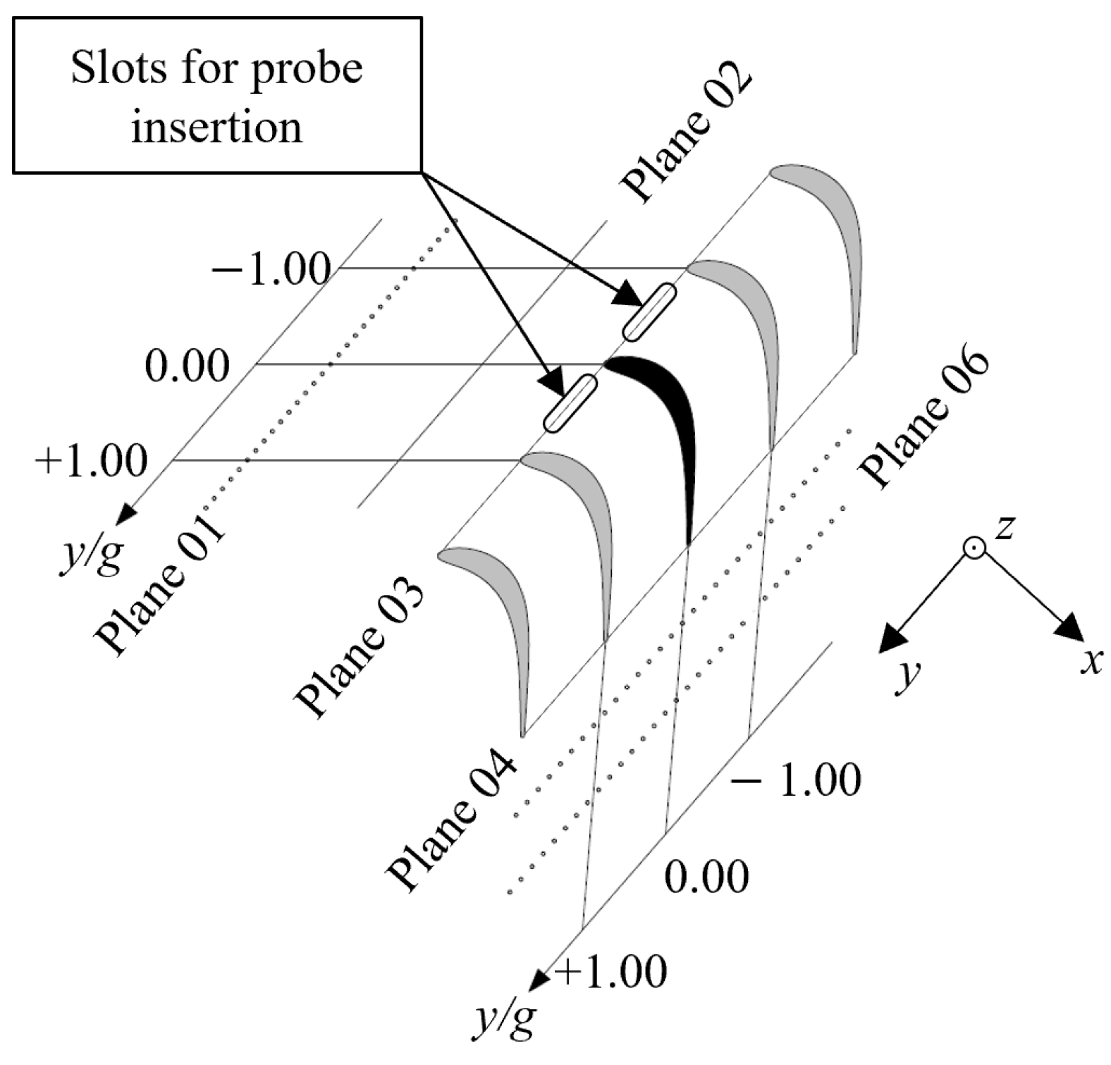
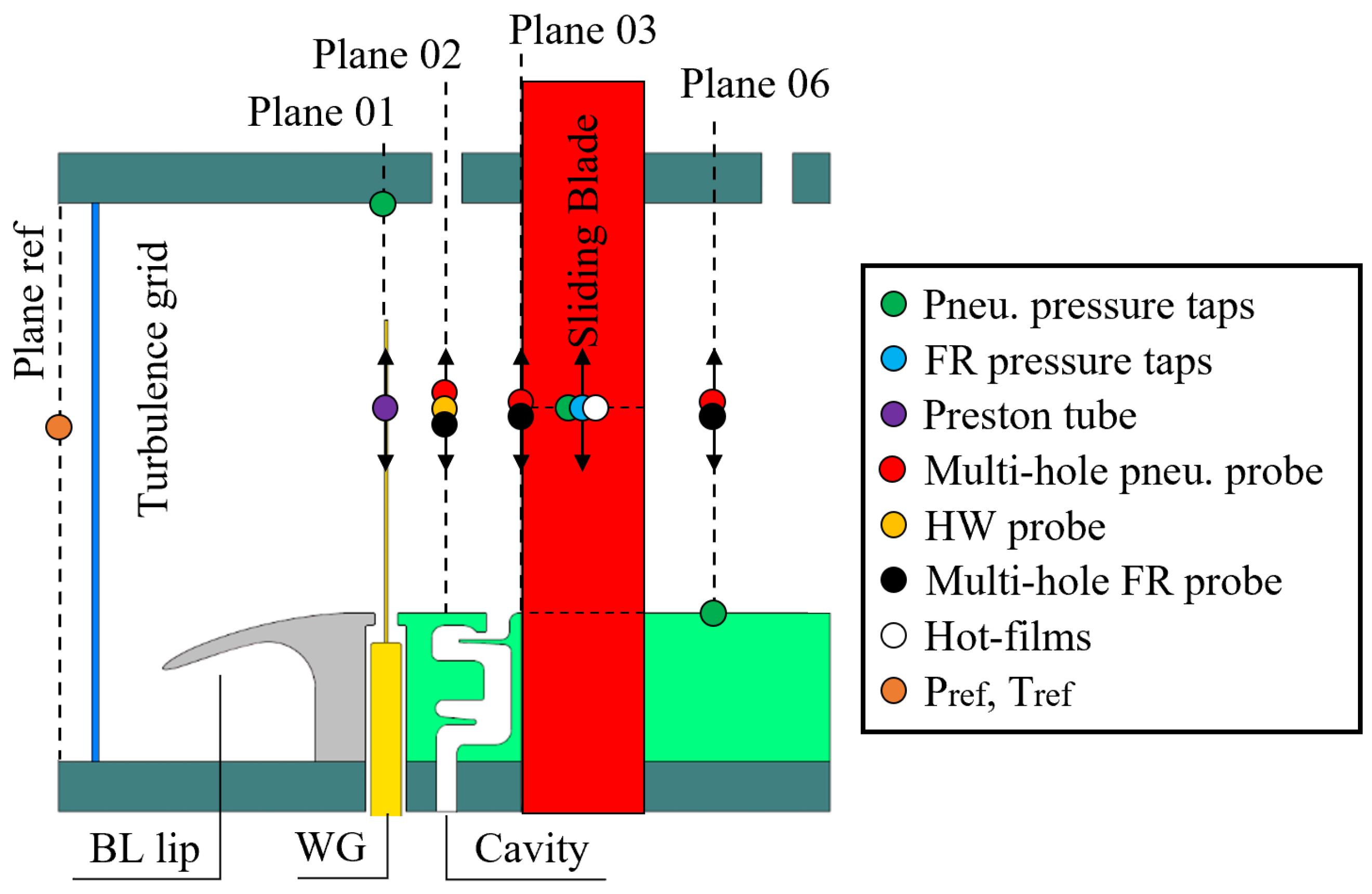
The test section was significantly redesigned to enhance its ability to test quasi-3D flows in a linear cascade setup. This redesign allowed for the characterization of profile aerodynamics and secondary flows in low-pressure turbine blades operating at engine-relevant Mach and Reynolds numbers while considering the combined effects of unsteady wakes and purge flows. The project introduced the concept of a sliding instrumented blade (see Section 4.2.3) to traverse the sensor location from midspan to the endwall.

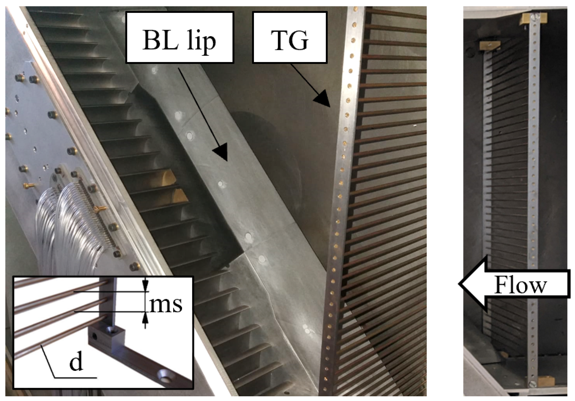
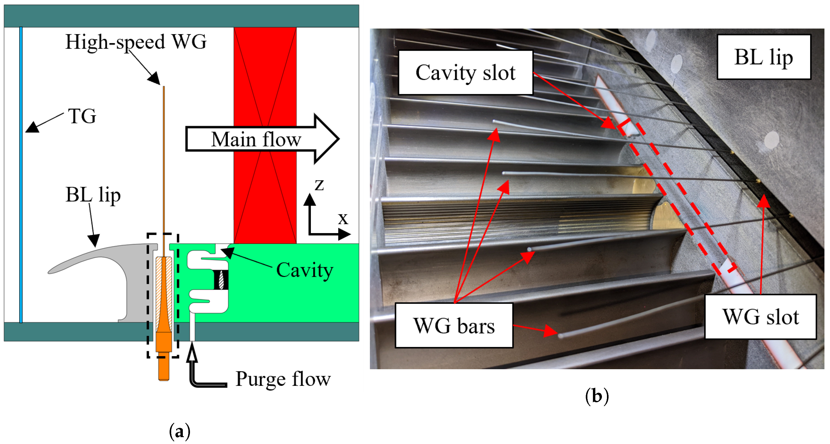
The adaptation involved translating one of the endwalls to accommodate the cavity geometry. This modification required the addition of a passive boundary layer control feature consisting of a splitter plate with a downward twisted leading edge. A super-elliptical leading edge [39] was employed to prevent separation and reduce sensitivity to incidence angles. The distance between the lip leading edge and the cascade leading edge was kept constant in order to maintain uniform boundary layer development across the pitchwise direction. The boundary layer lip is highlighted in Figure 4.

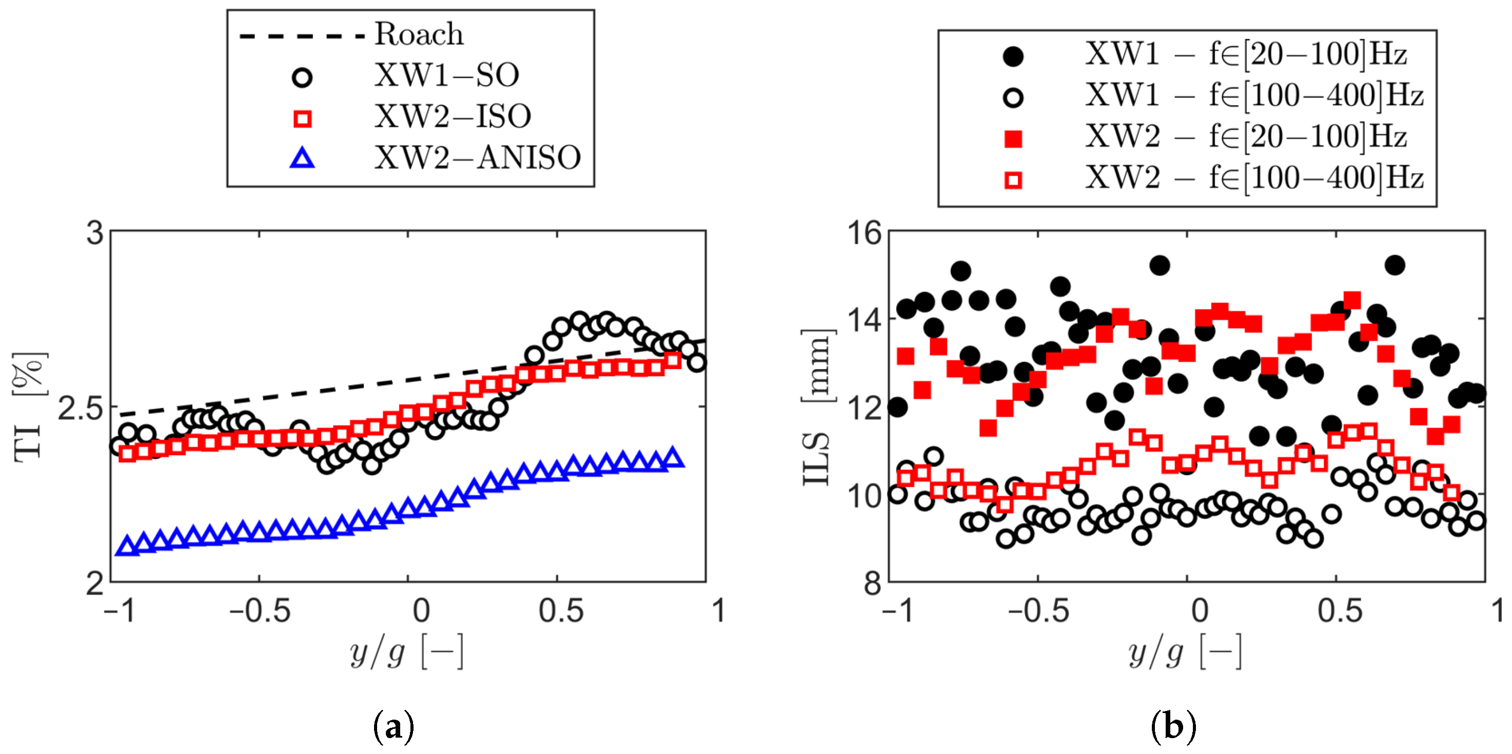
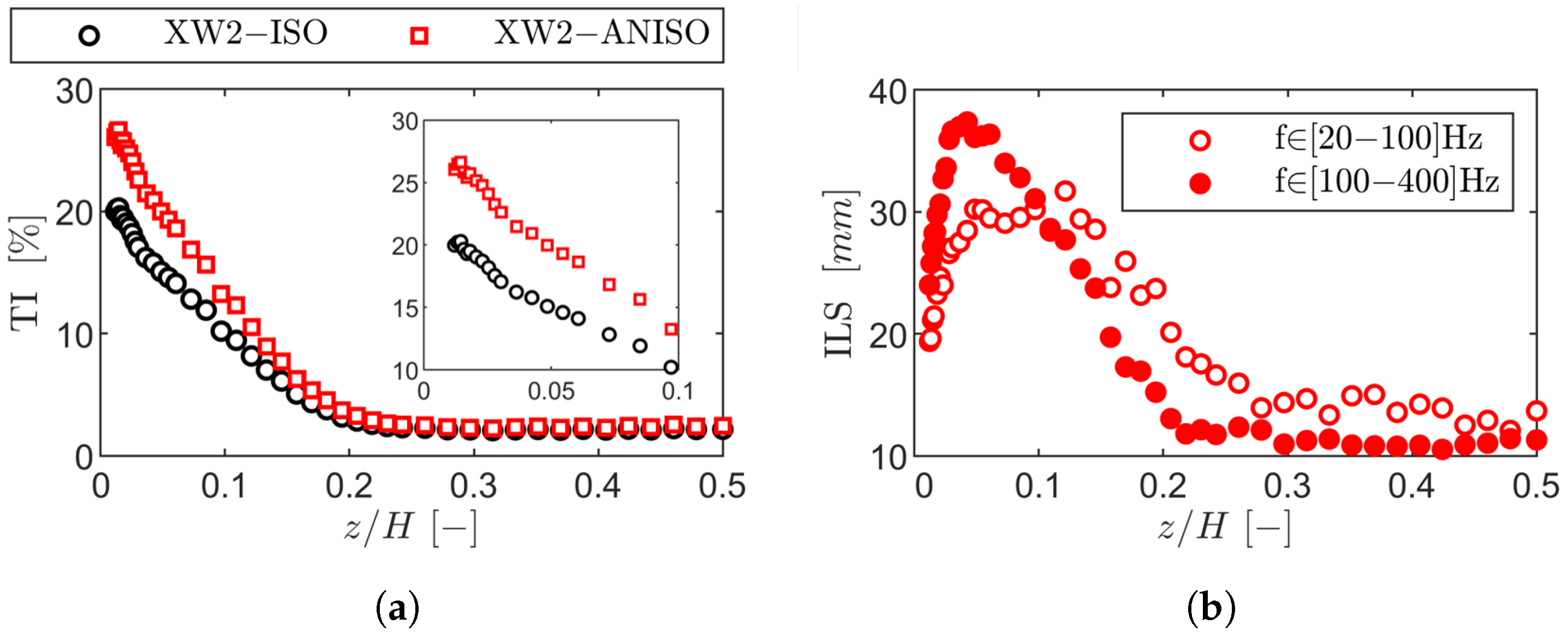
A passive turbulence grid was used to increase the turbulence level in the test section. This grid consists of an array of parallel cylindrical bars with a diameter of 2 mm and a mesh size of 12 mm. The correlation of Roach [40] was applied to determine the axial distance between the central blade and the turbulence grid. Positioned 400 mm upstream of the cascade central blade leading edge, the grid produced a turbulence level of approximately 2.4%. Hot-wire experiments were conducted to validate the correlation and assess turbulence decay upstream of the cascade (see Section 5.1). The position of the turbulence grid relative to the cascade is highlighted in Figure 4.

Tests concerning unsteady effects used a spoked wheel-type wake generator (WG) featuring 96 cylindrical bars with a diameter of 1.00 mm. The wake generator bars sit 1.12 axial chords upstream of the cascade leading edge plane. As suggested by Pfeil et al. [41], the bar diameter was selected to be similar to the blade trailing edge thickness in order to ensure a far wake similar that shed by an airfoil. The bars extended to ∼73% of the cascade span when parallel to the leading edge of the central blade.

Figure 5a schematically represents the test section constituents: the turbulence grid (TG), high-speed wake generator (WG), boundary layer (BL) lip, cavity geometry, and sliding blade. The assembled components within the VKI S-1/C are displayed in Figure 5b.

4. Experimental Methodology

4.1. Measurement Planes

The location of the measurement planes across the cascade is shown in Figure 6. At the cascade inlet, Plane 01 is aligned with the plane of rotation of the wake generator. Plane 02 is situated between the wake generator and the cascade LE. The blade row is constrained between Plane 03 at the LE and Plane 04 at the TE. Plane 05 and Plane 06 are used to characterize the outlet flow field. A reference plane not visible in Figure 6 sits far upstream of the turbulence grid, where the reference total pressure and temperature are measured. The location of the planes is reported in

Table 3. Location of measurement planes as a function of the axial chord.

Upstream of LE		Blade		Downstream of TE
Plane 01	Plane 02	Plane 03	Plane 04	Plane 06
$-1.12C_{ax}$	$-0.50C_{ax}$	$0.00C_{ax}$	$1.00C_{ax}$	$1.50C_{ax}$

.

4.2. Instrumentation

The cascade was heavily instrumented to collect flowfield measurements at the inlet (Planes 01, 02, 03) and outlet (Plane 06). Measurements on the blade and endwall surfaces were also performed. Figure 7 highlights the location and density of instrumentation used throughout SPLEEN.

Table 4. Types of instrumentation used for aerothermal measurements.

Instrumentation	Aerothermal Quantities
Pneumatic pressure taps	Time-averaged surface static pressure
FR pressure taps	Time-resolved surface static pressure
Preston tube	Time-averaged total pressure
Multi-hole pneu.probe	Time-averaged yaw angle, pitch angle, total pressure, static pressure, and Mach number
HW probes	Turbulence intensity and integral length scale
Multi-hole FR probe	Time-resolved yaw angle, pitch angle, total pressure, static pressure, and Mach number
Surface mounted hot-films	Quasi-wall shear stress, statistical moments of heat flux
${\mathrm{P}}_{ref}$, ${\mathrm{T}}_{ref}$	Reference inlet total pressure, and temperature

summarizes the purpose of the measurement techniques employed through the experimental campaign.

4.2.1. Cascade Fixed Instrumentation

Reference measurements of total pressure (${\mathrm{P}}_{0,ref}$) and total temperature (${\mathrm{T}}_{0,ref}$) are taken upstream of the turbulence grid. Two Pitot tubes placed at 30% and 50% of the total channel height upstream of the test section acquire the inlet reference total pressure, ensuring no spanwise pressure gradient. The readings are averaged. The reference pressure is measured with a WIKA P-30 absolute pressure sensor with an absolute range of 25 kPa. A K-type bare thermocouple positioned upstream of the pressure probes measures the reference temperature in a low-velocity region to maximize temperature recovery.

Static pressure in the test section is monitored using time-averaged pneumatic pressure taps along the endwalls at Planes 01, 03, and 06. At Plane 01, 31 static pressure taps are evenly distributed across three pitches in the pitchwise direction. Plane 03 has 14 taps, while Plane 06 features 31 taps across four pitches. The far exit static pressure is monitored to maintain stable operating conditions free from probe blockage effects [42,43] and independent of the cascade outlet flow. Two Scanivalve MPS4264 miniaturized piezoresistive pressure units, each with 64 channels and ranges of 1 psi and 2.5 psi, are used to record surface static pressure.

4.2.2. Aerodynamic Probes

The flowfield was surveyed using pneumatic and fast-response aerodynamic probes. The probes are shown in Figure 8. The probes were traversed in the test section using a carriage system that provided pitchwise and spanwise motion and rotation around the probe axis. The linear resolution of the traversing system is ∼0.05 mm, while the smallest achievable rotation is ∼0.10°.

A Preston boundary layer tube (PT) measures the inlet total pressure profile at Plane 01. An aspect ratio (W/H) of 2.60 characterizes the probe head. The probe head is aligned with the inlet metal flow angle. For a conventional round Pitot tube, the insensitivity range to the inlet flow angle is ±11$°$ for Mach numbers ranging from 0.26 to 1.62 [44]. It is assumed that the range of a flat-head Pitot probe (Preston tube) is similar. Based on the aspect ratio of the Preston tube head and the flow conditions measured in the VKI S-1/C, a maximum error of 0.1% of the inlet freestream total pressure is expected due to the “Barker effect” [45].

A second source of error is attributable to wall proximity. This effect is reported in [46] for circular Pitot tubes. The error becomes non-negligible for distances to the endwall below two probe head diameters (z/D < 2). Based on the hydraulic diameter of the Preston tube head and the flow conditions investigated in the scope of this work, the maximum error in the velocity due to the wall proximity effect is 0.6% of the inlet freestream isentropic velocity. This effect is assumed to have the same magnitude for flattened Pitot tubes (Preston tubes). For this reason, no correction was applied. The Preston tube is connected to the Scanivalve MPS4264–1 psi. During testing, the signal is sampled at 300 Hz for a sampling time of 3 s.

Two hot-wire probes were used at Plane 02 to survey the freestream turbulence. Both probes were operated using constant temperature anemometry (CTA). A cross-wire probe (XW) was used in the absence of the wake generator, and a single-wire (HW) was used to measure downstream of the wake generator. A detailed description of both the probes and the methodology employed for obtaining measurements in transonic rarefied flowfields can be found in [47], and followed refinement of the technique throughout the experimental campaign. The output voltage was acquired at 100 kHz for 3 s and low-pass filtered at 30 kHz via an analog filter before being digitized by a 16-bit NI card.

Two miniaturized five-hole probes were used to obtain the flow angle, total pressure, and static pressure. At Plane 02, a cobra-shaped five-hole probe (C5HP) is used, while an L-shaped five-hole probe is used at Plane 06. Both use aerodynamic coefficients proposed by Treaster [48] to retrieve local aero-thermodynamic quantities based on the tap readings. The tap nomenclature for the L5HP and C5HP is displayed in Figure 8.

$$K_{\alpha }\left(\alpha ,\gamma ,M\right)={\displaystyle \frac{P_L-P_R}{P_C-P_{ave}}}$$

(3)

$$K_{\gamma }\left(\alpha ,\gamma ,M\right)={\displaystyle \frac{P_D-P_U}{P_C-P_{ave}}}$$

(4)

$$K_{tot}\left(K_{\alpha },K_{\gamma },M\right)={\displaystyle \frac{P_C-P_0}{P_C-P_{ave}}}$$

(5)

$$K_{stat}\left(K_{\alpha },K_{\gamma },M\right)={\displaystyle \frac{P_{ave}-P}{P_C-P_{ave}}}$$

(6)

$$P_{ave}=\left(P_L+P_R+P_D+P_U\right)/4$$

(7)

The C5HP is characterized by a pyramidal head shape with a diagonal of 1.80 mm. The probe was used in non-nulled (calibrated) mode. An aerodynamic calibration in an open jet was performed to investigate the angular sensitivity of the probe at different flow Mach numbers. The probe has been calibrated for yaw and pitch angles in the range of ±30$°$ and ±20$°$ in increments of 1$°$, respectively. The angular sensitivity of the probe to the incoming flow field was investigated for flow Mach numbers of 0.20, 0.40, and 0.60 to cover the expected range of Mach numbers at the inlet of the cascade for the current investigation. As proposed by [49], an iterative procedure retrieves the local aero-thermodynamic quantities from the aerodynamic coefficients. The taps are connected to the Scanivalve MPS4264–1 psi. During testing, the signal is sampled at 300 Hz for a sampling time of 3 s.

The Reynolds numbers differed between calibration (Re > 8000) and testing (1500–2600). According to Passman et al. [50], the calibration coefficients of pyramidal-shaped multi-hole probes will be maintained down to a critical Reynolds number of ∼11,000. In the scope of this work, it was not possible to quantify the impact of the Reynolds number on the measurements.

The L5HP is characterized by a hemispherical head with a diameter of 2.20 mm. The probe was calibrated in an open jet for a range of yaw and pitch angles between ±30$°$ and for M ∈ {0.20, 0.40, 0.60, 0.80, 0.90, 0.95}. The Reynolds number based on the probe head diameter during testing was ∼3000; therefore, Reynolds effects on the aerodynamic calibration are assumed to be negligible [51]. The taps are connected to the Scanivalve MPS4264–1 psi. During testing, the signal is sampled at 300 Hz for a sampling time of 3 s. Before acquisition, the probe rests at the measuring location for 8 s to ensure that the pressure has settled.

The FRV4HP design was inspired by that in [52,53]. The redesigned probe with commercially available fast-response sensors has a head diameter of 2.65 mm. The probe measures at Planes 02, 03, and 06. It is instrumented with two Kulite LQ-062-5A sensors with an absolute range of 35 kPa. Figure 9 schematically highlights the position of the sensors in the probe head.

The sensors are recessed from the probe surface to increase spatial resolution. It is estimated that the design provides a bandwidth of over 30 kHz according to the model of Helmholtz [54] and Bergh and Tijdeman [55]. Due to the low range of the sensors, no dynamic calibration was performed. The probe underwent aerodynamic calibration in an open jet for a range of yaw and pitch angles between ±70$°$ and ±30$°$, respectively. The probe was calibrated for M ∈ {0.20, 0.40, 0.60, 0.80, 0.90, 0.95}.

The probe is operated in virtual mode [52,56,57]. A virtual displacement of ±30$°$ is used. The coefficients proposed by Pfau et al. [56] are used to retrieve the flow angles, $\alpha$, and local total pressure based on the tap readings. The tap nomenclature for the FRV4HP is displayed in Figure 8.

$$K_{\alpha }\left(\alpha ,\gamma ,M\right)={\displaystyle \frac{P_L-P_R}{P_C-P_{ave}}}$$

(8)

$$K_{\gamma }\left(\alpha ,\gamma ,M\right)={\displaystyle \frac{P_D-P_C}{P_C-P_{ave}}}$$

(9)

$$K_{tot}\left(K_{\alpha },K_{\gamma },M\right)={\displaystyle \frac{P_C-P_0}{P_C-P_{ave}}}$$

(10)

$$P_{ave}=\left(P_L+P_R\right)/2$$

(11)

The signals were sampled by a NI6253–USB data acquisition board, acquired at 1200 kHz, and sampled for 3 s.

4.2.3. Blade Surface Measurements

The cascade consists of 23 blades, with five variations of the central blade used during the experimental campaign. A smooth central blade is mounted for probe measurements to ensure that the sensors do not impact the cascade loss. A sliding instrumented blade was designed to measure the pressure and quasi-wall shear stress from the midspan to the endwall. The instrumented blades move across this range, allowing the sensor array to cover the area from endwall to midspan. The set of instrumented blades includes an instrumented blade with 24 pneumatic taps on the suction side, an instrumented blade with seven fast-response Kulite LQ062–5 psi on the suction side, an instrumented blade with 17 pneumatic taps and one Kulite LQ062–5 psi on the pressure side, and an instrumented blade with 32 hot-film (HF) sensors on the suction side and 21 on the pressure side.

The location and dimensions of the taps on the blade surfaces are shown in Figure 10. To maintain mechanical integrity, the diameter of the pneumatic taps varies between 0.3 and 0.8 mm. Recessed absolute transducers (Kulite LQ062) with a 5 psi range are installed beneath the surface.

The blade is equipped with pressure taps on the pressure side and includes a fast-response pressure transducer. Figure 10 shows the location of the fast-response pressure taps on the suction side. The blade sensors have been recessed to improve spatial resolution, reducing the sensing tap area from 1.70 mm to 0.60 mm. The most critical line–cavity geometry occurs at the leading edge sensor. Acoustic models by Helmholtz [54], Hougen [58], and Bergh and Tjideman [55] indicate that the lowest bandwidth exceeds 36 kHz, which is sufficient to capture up to five harmonics of the bar passing frequency during tests with the wake generator. Each sensor was sampled using a NI6253–USB data acquisition board at 1.2 MHz for 3 s. Signals were filtered with a 250 kHz analog low-pass filter before acquisition.

Senflex^® surface-mounted hot-films were used for blade measurements. Nickel sensor elements and copper leads were printed on Upilex S polyamide film^®. The sensor geometry consists of a sensing element measuring 0.1016 mm × 0.0002 mm × 1.4478 mm in width, thickness, and length, respectively. A cold resistance of approximately $9.90 \mathrm{\Omega }$ was measured at 20 °C for all sensors. The leads measure 0.60 mm × 0.0127 mm × 215 mm. The array contained 31 sensors on the suction side and 21 on the pressure side, which were spaced 2 mm apart. A hot-film array designed in-house and produced by Tao Systems was wrapped around the leading edge and recessed on both the suction and pressure sides to ensure a smooth blade profile without steps.

Actuated by a servomotor, a newly designed traversing unit moves the instrumented blades along the span with a 0.05 mm resolution. A 0.05 mm clearance in a 3D-printed insert within the cascade casing minimizes friction and prevents leakage from the test section. The blade traversing system is illustrated in Figure 10.

4.2.4. Endwall Measurements

The two passages adjacent to the central blade are instrumented on the lower endwall with pneumatic and fast-response pressure taps and surface-mounted hot-film sensors. The pneumatic and fast-response taps are integrated into two inserts on the endwalls: Insert 1 above the central blade, and Insert 2 below it. Insert 1 contains thirty pneumatic taps and six fast-response taps, while Insert 2 holds thirty-six pneumatic taps and two fast-response sensors. Fast-response taps are equipped with Kulite XCQ-062 5 psi sensors. The inserts and the location of the taps within the passage are shown in Figure 11.

Two inserts with hot-film sensors were manufactured to conduct HF measurements on the cascade endwalls. The flow between the two blade passages adjacent to the central blade was assumed to be periodic, allowing for an even distribution of sensors between the inserts. Each passage was equipped with 24 sensors. As presented by Vera et al. [59], sensors were positioned along the passage trajectory. As with the blade, Tao Systems designed and manufactured a custom Senflex^® hot-film array in-house. The nickel sensor elements and copper leads were printed on a Upilex S polyamide film^®.

4.3. Measurement Uncertainty

The measurement uncertainty was evaluated using the ASME method [60], with errors categorized as “random” if they varied during measurement and “systematic” if they remained constant. The non-propagated total uncertainty of a measured quantity was estimated according to Equation (12).

$$U_{tot}=\sqrt{U_{sys}^2+U_{rand}^2}$$

(12)

The expanded uncertainty with a 95% confidence interval can be computed as follows:

$$U_{tot,95\%}=\pm t_{95}\left(\nu \right)\times U_{tot}$$

(13)

where $t_{95}\left(\nu \right)$ is the Student t-distribution and relies on the combined degrees of freedom of the measured quantity. In the scope of this work, the degrees of freedom for systematic uncertainty were assumed to be infinite. For quantities deriving from signals, at least 600 samples were used. There are enough degrees of freedom to consider $t_{95}\left(\nu \right)=2$ in the scope of this work.

For a generic quantity q that is a function of n independent parameters,

$$q=f({\mathsf{\Phi }}_1,{\mathsf{\Phi }}_2,{\mathsf{\Phi }}_3,\dots ,{\mathsf{\Phi }}_n).$$

(14)

The uncertainty propagation into the derived quantity q due to the uncertainty of its parameters is determined through a Taylor series method (TSM) by neglecting higher-order terms:

$$U_q=\sqrt{\sum _{n=1}^n{\left({\displaystyle \frac{\partial q}{\partial {\mathsf{\Phi }}_i}}\right)}^2}.$$

(15)

The $\partial q/\partial {\mathsf{\Phi }}_i$ represents the sensitivity coefficient expressing the dependence of ${\mathsf{\Phi }}_i$ on q.

Table 5. Breakdown of experimental uncertainty with 95% confidence interval.

Quantity	Symbol	Unit	Value	${\mathit{U}}_{\mathbf{rand}}$	${\mathit{U}}_{\mathbf{sys}}$
Fixed instrumentation/Blade/Endwalls-Pneumatic
Inlet total temperature	$T_{ref}$	K	304.90	0.002	0.518
Isentropic Mach number	$M_{is}$	-	0.905	0.0007	0.0054
Isentropic Reynolds number	$R{e}_{is}$	-	71,611	59	1438
Strouhal number	$f^{+}$	-	0.94	0.0007	0.0185
Purge massflow rate	PMFR	Abs. %	0.90	0.0020	0.0020
Blade-Fast-Response
Norm. pressure fluctuations	$\Delta P/P_{01}$	-	0.100	0.000	0.004
Preston tube
VBL over Vfs	$V_{BL}/V_{fs}$	-	1.000	0.001	0.008
Derived Quantities
Turbulence grid loss coeff.	$Y_{TG+WG}$	-	0.0590	0.00070	0.00174
Inlet total pressure-Correlation	$P_{01}$	$Pa$	9901	7.09	29.82
With C5HP
Inlet Primary flow direction	${\beta }_{in}$	$°$	35.18	0.24	0.96
Inlet cascade pitch angle	${\gamma }_{in}$	$°$	1.02	0.24	0.73
P02 over P01	$P_{02}/P_{01}$	-	1.0005	0.001	0.005
P2stat over P01	$P_2/P_{01}$	-	0.8774	0.001	0.004
With FRV4HP
Inlet Primary flow direction	${\beta }_{in}$	$°$	35.18	0.23	1.65
Inlet cascade pitch angle	${\gamma }_{in}$	$°$	1.02	0.24	2.75
Outlet Primary flow direction	${\beta }_{out}$	$°$	51.76	0.16	1.00
Outlet cascade pitch angle	${\gamma }_{out}$	$°$	−0.52	0.13	1.24
Energy loss coefficient	$\xi$	-	0.1500	0.0023	0.0114
With L5HP
Outlet Primary flow direction	${\beta }_{out}$	$°$	51.7601	0.15	0.33
Outlet cascade pitch angle	${\gamma }_{out}$	$°$	−0.5188	0.13	0.21
Energy loss coefficient	$\xi$	-	0.1500	0.0019	0.0095
Hot wire anemometry
Turbulence intensity	TI	% u	2.40	-	0.20%
Integral length scale	ILS	mm	12	-	3.92

shows the expanded uncertainty and typical values of key quantities acquired during the experimental campaign. Systematic errors are the main contributors to overall uncertainty; however, differences in measurements across operating points (exit Mach and Reynolds numbers) or at different pitch and span locations were minimally affected by systematic errors. The same calibrated transducers and measurement chains were used in a stable experimental setup [61]; thus, the uncertainty in comparing measurements was mainly due to random errors, with minimal systematic uncertainty. A detailed breakdown of uncertainty sources and expanded uncertainty for other derived quantities not reported here is provided in [36].

5. Rig Commissioning

The rig was commissioned to ensure stable and robust operation throughout the campaign via inlet flow characterization, operating point stability, outlet periodicity, and probe interference [42].

5.1. Turbulence Intensity

Michálek et al. [62] reported a natural freestream turbulence intensity of 0.9% in the VKI S-1/C. The turbulence profile was recharacterized both with and without the turbulence grid in the absence of the wake generator. Pastorino et al. [47] measured the inlet turbulence with the wake generator.

The hot-wire technique used for low-density transonic flows for tests performed in the VKI S-1/C has been developed since 2020. Figure 12a shows the pitchwise distributions of turbulence intensity measured during the experimental campaign, with the decay correlation by Roach [40] included for comparison. Turbulence decays toward negative pitchwise locations due to the increased axial distance from the turbulence grid. The correlation of Roach closely matches the data. The “XW1-ISO” measurements were taken in 2023 [47] assuming isotropic flow (${V_x}^{\prime }={V_y}^{\prime }={V_z}^{\prime }$):

$$T{I}_{iso}={\displaystyle \frac{\sqrt{\frac{1}{3}\left({V_x}^{\prime 2}+{V_y}^{\prime 2}+{V_z}^{\prime 2}\right)}}{\overline{V}}}={\displaystyle \frac{\sqrt{{V_x}^{\prime 2}}}{\overline{V}}}.$$

(16)

By performing an extensive in situ calibration of the probe, recent developments in early 2024 have allowed for the measurement of streamwise and crosswise components (“XW2-ANISO”) according to Equation (18). The third component of the velocity fluctuations is not neglected; instead, it is assumed to be the mean between the sum of the squares of the streamwise and pitchwise components.

$${V_z}^{\prime 2}={\displaystyle \frac{{V_x}^{\prime 2}+{V_y}^{\prime 2}}{2}}$$

(17)

$$T{I}_{aniso}={\displaystyle \frac{\sqrt{\frac{1}{2}\left({V_x}^{\prime 2}+{V_y}^{\prime 2}\right)}}{\overline{V}}}$$

(18)

For completeness, data obtained from the latest measurements assuming the flow to be isotropic are also included (“XW2-ISO”). Although both profiles show similar decay, the turbulence computed with multiple components is 0.27% lower. Similar decay trends are confirmed by the pitchwise distribution of the integral length scale shown in Figure 12b. The length scale remains relatively constant across the pitchwise range, supported by the similar slope of the turbulence intensity decay. The length scale is computed based on the spectrum integration method provided in [40]:

$$ILS=\overline{V}{\left[{\displaystyle \frac{E\left(f\right)}{4\overline{{V^{\prime }}^2}}}\right]}_{f\to 0Hz}.$$

(19)

A length scale of ∼12 mm was obtained by integrating the streamwise velocity spectrum between 20–100 Hz. Changing the integration limit to the range of 100–400 Hz results in a similar length scale of ∼10 mm. The integral length scale measured with the grid is comparable to the turbulent grid mesh size. The power law described by Roach [40] was used to fit the turbulence intensity decay:

$$TI=A{\left({\displaystyle \frac{x}{d}}\right)}^B.$$

(20)

The axial distance to the turbulence grid is represented by x, while d represents the turbulence grid bar diameter.

Table 6. Power law coefficients fitted to HW data.

Model/Instrumentation	A	B
Roach [40]	0.800	−0.714
XW1-ISO	0.771	−1.178
XW2-ISO	0.804	−1.112
XW2-ANISO	0.677	−1.173

compares the coefficients of the fitted curves against those in [40] for turbulence grids made of an array of cylindrical parallel rods.

Figure 13a displays the radial profiles of the turbulence intensity and integral length scale measured with the cross-wire probe at Plane 02 in the absence of incoming wakes.

The turbulence intensity reports the quantity computed under isotropic turbulence assumption (XW2-ISO) and by accounting for the streamwise and crosswise components (XW2-ANISO). For both of these, the turbulence is found to increase towards the endwall. For the anisotropic case, the turbulence reaches values as high as 26%. The anisotropic turbulence is higher than the isotropic turbulence along the span, being 32% higher at the closest point to the endwall.

The radial distribution of the integral length scale is displayed in Figure 13b. The length scale was obtained by integrating the spectrum in the 20–100 Hz and 100–400 Hz ranges, as was done for the pitchwise measurements. Both methods resulted in an increased length scale in the boundary layer region. The peak is followed by a decrease towards the endwall, where the length scale is ∼20 mm. Using the 100–400 Hz integration range displays a sharper peak at z/H = 0.05.

5.2. Turbulence Grid Total Pressure Loss Correlation

The inlet total pressure is not live-monitored during tests, as placing a probe between the turbulence grid and wake generator is impractical with the current setup. Instead, a loss coefficient Y is defined across the turbulence grid or both the grid and wake generator, as shown in Equation (21):

$$Y\left(M,Re\right)={\displaystyle \frac{P_{0,ref}-P_{01,fs}}{P_{0,ref}}}.$$

(21)

When Y is known for a given flow condition, the total pressure at the cascade inlet (downstream of the turbulence grid and wake generator, if present) can be obtained by isolating $P_{01,fs}$ in Equation (21), as $P_{0,ref}$ is live-monitored.

A correlation for the loss across the turbulence grid, including the wake generator for tests with bars, was developed by testing across expected flow conditions. A probe was installed to measure the total pressure at the cascade inlet in order to calculate Y. Using only the turbulence grid, the total pressure was retrieved at Plane 01 using a Preston tube. When the turbulence grid and wake generator were installed, the total pressure was measured at Plane 02 using a Cobra five-hole probe. Figure 14 displays the pitchwise distributions of the total pressure loss coefficient for the range of flow conditions investigated. The pitch-to-pitch variation is within ±0.10% of the inlet freestream total pressure.

The loss coefficient distributions were averaged pitchwise for each flow condition to obtain a loss correlation as a function of Mach and Reynolds numbers. The loss correlations for the cases with turbulence grid and with turbulence grid in addition to the wake generator take the following form:

$$Y\left(M_{6,is},{Re}_{6,is}\right)=C_1+C_2{M}_{6,is}+C_{3}R{e}_{6,is}+C_4{M}_{6,is}^2+C_4{M}_{6,is}R{e}_{6,is}.$$

(22)

The coefficients of the fittings alongside the goodness of fitting and fitting error are displayed in

Table 7. Calibration coefficients, goodness of fitting, and standard error of fittings for correlations of outlet flow conditions.

Coefficients	${\mathit{Y}}_{\mathit{TG}}$	${\mathit{Y}}_{\mathit{TG}\mathbf{+}\mathit{WG}}$
$C_1\left[-\right]$	−0.05513	−0.05349
$C_2\left[-\right]$	0.18825	0.22443
$C_3\left[-\right]$	5.04960 × ${10}^{-8}$	1.13957 × ${10}^{-7}$
$C_4\left[-\right]$	−0.09340	−0.10919
$C_5\left[-\right]$	−4.53216 × ${10}^{-8}$	−1.32206 × ${10}^{-7}$
$R^2\left[-\right]$	0.99953	0.99907
$S_{\overline{\mathbb{M}}}\left[-\right]$	6.44884 × ${10}^{-8}$	3.58202 × ${10}^{-7}$

.

In addition, correlations based on the inlet Mach and Reynolds were built. The reader is referred to [36] for a detailed description. The final maps resemble those shown for the case with turbulence grid in Figure 15. The loss mainly depends on the Mach number, and is nearly insensitive to the Reynolds number.

5.3. Operating Conditions Stability

The stability of the rig operating conditions was evaluated during each testing phase, spanning multiple days of data collection. Due to the intrusiveness of the L-shaped five-hole probe at Plane 06 [42], stability in terms of Mach and Reynolds numbers was assessed using the static pressure at the cascade far exit. As temperature variations during testing could reach 8 K, the rig was adjusted to maintain constant Mach and Reynolds numbers.

Flow stability was quantified using the standard deviation of the probability density function for each parameter.

Table 8. Repeatability of the cascade operating conditions with 95% confidence interval resulting from variation in flow conditions from the nominal point.

Phase		1	2	3
WG		-	X	X
Purge		-	-	X
M	rel $[\%]$	0.71	0.92	0.71
	abs $[-]$	0.006	0.008	0.006
Re	rel $[\%]$	0.61	0.71	0.82
	abs $[-]$	425	500	574
RPM	rel $[\%]$	-	0.004	0.003
	abs [rpm]	-	0.12	0.11
$f^{+}$	rel $[\%]$	-	0.54	0.30
	abs $[-]$	-	0.005	0.003
PMFR 0.50%	abs $[\%]$	-	-	0.002
PMFR 0.90%	abs $[\%]$	-	-	0.003

summarizes the standard deviation with a 95% confidence interval ($2\sigma$) for Mach and Reynolds numbers, wake generator rotational speed, bar reduced frequency, and purge massflow ratio across all testing phases. Both percentage and absolute values for the nominal operating point (M = 0.90, Re = 70k, St = 0.95) are provided.

5.4. Inlet Boundary Layer

The inlet boundary layer periodicity was measured at Plane 01 using the Preston tube for the nominal operating point. Figure 16 shows the inlet total pressure profiles at various pitchwise locations. There is virtually no difference between the profiles. The maximum variation occurs near the endwall, and is approximately 0.10% of the inlet total pressure.

The pitch-to-pitch periodicity of the boundary layer was also assessed using boundary layer integral parameters. Figure 17a shows the pitchwise distribution of the normalized displacement thickness, with variations within ±0.35 mm. The momentum thickness (Figure 17b) varied by ±0.26 mm. As both quantities decrease with pitchwise location, the shape factor remains nearly constant, as shown in Figure 17c, indicating a fully turbulent boundary layer at Plane 01 [63].

Regarding the influence of inlet boundary layer periodicity on secondary flow development across the cascade, the displacement thickness increases by approximately ∼53% toward the negative passages. Based on the Coull and Clark model [23], this increase is expected to result in the loss increasing by about 2.60%.

The zigzag pattern observed here results from the specific probe traversing trajectory used during measurements. The probe was first moved pitchwise, then away from the endwall, and then pitchwise again until midspan, with the inlet and outlet maps constructed by stacking multiple pitchwise traverses. Boundary layer measurements were performed early in the campaign using successive spanwise traverses in which the probe moved in the opposite spanwise direction at adjacent pitchwise locations relative to the previous traverse. The fluctuations arose from the probe entering and leaving the low-momentum boundary layer region, along with a less meticulous analysis of probe settling time.

5.5. Inlet Flow Periodicity

The periodicity of the inlet boundary layer was also characterized at Plane 02 with and without the wake generator. The effect of purge flow on periodicity is discussed in [30]. Cobra five-hole probe measurements captured the periodicity in terms of angles and the total pressure profile. Figure 18 shows the radial profile at different pitchwise locations at Plane 02 without the wake generator.

Figure 18a shows the incidence, which decreases with pitchwise location. The variation at y/g = 0.00 is within ±1.60$°$ near the endwall, and is three times lower at midspan. The cascade pitch angle (Figure 18b) shows a non-monotonic variation, with the central location varying by ±0.25$°$ near the endwall. The normalized total pressure profile (Figure 18c) shows a maximum pitch-to-pitch variation of ±0.005 near the endwall and ±0.001 at midspan.

Figure 19a shows the radial incidence profiles at Plane 02 with the wake generator. The incidence increases with pitchwise location, with variation within ±0.10$°$ at midspan and exceeding ±2.00$°$ below z/H=0.05 near the endwall. The cascade pitch angle (Figure 19b) was affected by the wake generator at midspan, with variation within ±0.40$°$ across the span. Figure 19c displays the radial profiles of the normalized total pressure, showing higher loss towards negative pitchwise locations. The pitch-to-pitch variation is within ±0.1% of the inlet total pressure at midspan, but reaches ±1.25% near the endwall.

5.6. Outlet Flow Periodicity

The periodicity at Plane 06 was surveyed over the range y/g ∈ [−1.50, +1.50]. To ease comparison, the flow domain includes three blade wakes shifted by one blade pitch. Without the wake generator or purge flow, measurements were performed at targeted spanwise locations of z/H ∈ {0.01, 0.05, 0.10, 0.50} rather than mapping the whole flow domain. Figure 20a displays the pitchwise mass-averaged primary flow direction for the investigated pitches, defined as $\beta ={tan}^{-1}\left(V_{tan}/V_{ax}\right)$. The differences are within ±0.30$°$. Similar findings are reported for the cascade pitch angle defined as $\gamma ={tan}^{-1}\left(V_r/V_{ax}\right)$ (see Figure 20b). Figure 20c shows the mass-averaged kinetic energy loss coefficient, defined as follows:

$$\xi =1-{\displaystyle \frac{1-{\left(\frac{P_6}{P_{06}}\right)}^{\frac{\gamma -1}{\gamma }}}{1-{\left(\frac{P_6}{P_{01}}\right)}^{\frac{\gamma -1}{\gamma }}}}.$$

(23)

The pitch-to-pitch variation at midspan is within ±0.002. At z/H = 0.05, the pitch-to-pitch variation of the kinetic energy loss coefficient is within ±0.006.

The loss variation across different passages results from pitchwise variations in inlet boundary layer thickness. A thicker boundary layer increases secondary losses due to the larger vorticity extent processed within the cascade passage [23].

The variation in mass-averaged loss is better understood through the pitchwise distribution of $\xi$ at different spanwise locations in Figure 21. The pitchwise coordinate ${\mathrm{y}}^{*}$ reflects a re-shift by one blade pitch, with the origin at the intersection of the outlet metal angle and Plane 06. At z/H = 0.05, variation increases away from the loss peak. Loss variation between wakes is similar in the peak and freestream regions at the subsequent spanwise locations. The outlet secondary flows do not influence the midspan, making the cascade outlet flow highly periodic in the 2D region. A slight discrepancy in the freestream region at ${\mathrm{y}}^{*}$/g = 0.40 arises from the inlet freestream total pressure used to estimate the kinetic energy loss coefficient, which is derived from the total pressure loss correlation based on a smaller pitchwise range than the outlet measurements (three blade passages).

Next, the periodicity was recharacterized with the introduction of the wake generator. Figure 22 shows contours for the three blade wakes in terms of the primary flow direction (Figure 22a) and kinetic energy loss coefficient (Figure 22b). The features are similar across all three wakes.

In the primary flow direction (Figure 22a), two distinct regions can be observed: underturning away from the endwall (“A”), and overturning near the endwall (“B”), which is mainly associated with the secondary flows. These regions intensify towards the passage above the central blade. Similar trends were observed in the cascade pitch angle (not shown).

The intensification of secondary flow structures is also evident in the kinetic energy loss coefficient (Figure 22b), with two loss cores identified. The core near the endwall (“F”) is in the corner vortex region, while the one away from the endwall (“E”) is due to the secondary flows. Both cores intensify towards negative pitchwise locations, with the displacement of the loss core away from the endwall caused by stronger secondary flow structures.

The thicker boundary layer towards negative passages again justifies the variation in loss across the passages. Increased boundary layer thickness leads to larger secondary loss due to the larger amount of vorticity processed by the cascade passage [23]. In addition, Walsh and Gregory-Smith [64] found that the inlet boundary layer skewness significantly modifies the inlet vorticity distribution, which impacts the secondary flow development. Negatively skewed boundary layers promote higher secondary loss. A more negative skewness characterizes the inlet boundary layer measured at y/g = −1.00 than at increasing pitchwise locations. As a result, the secondary loss is higher towards negative pitches.

The mass-averaged radial profiles show intensification of secondary flow structures and deeper penetration toward the passage center. Figure 23a shows a larger overturning near the endwall (“B”) by approximately 4.00$°$, while the underturning peak (“A”) increases by about 1.50$°$ and shifts away from the endwall.

The pitchwise averaging of the cascade pitch angle combines upwash and downwash regions, which cannot be decoupled. However, higher downwash intensity (“C” in Figure 23b) for wakes at y/g = −1.00 and y/g = 0.00 shows an increase in cascade pitch angle near the endwall, with a variation of around 1.50$°$.

The mass-averaged kinetic energy loss coefficient displayed in Figure 23c confirms these findings. The peak loss associated with the corner vortex (“F”) and passage vortex coupled with trailing shed vorticity (“E”) intensifies toward negative pitches, with an increase of 0.014 and displacement of the loss peak away from the endwall.

Despite the impact of the secondary flow structures on the mass-averaged quantities near the endwall, the midspan periodicity is characterized by the excellent agreement of the wake loss signature for the three measured wakes as displayed in Figure 24.

Periodicity was also investigated with purge flow and the wake generator. Figure 25 shows the flowfield in terms of the primary flow direction (Figure 25a) and kinetic energy loss coefficient (Figure 25b) for a purge massflow ratio of 0.90%. Similar flow features to those in Figure 22 can be observed, with increased intensity of secondary flow structures towards negative pitchwise locations. However, unlike the case without purge flow, there is no significant displacement of the secondary flow structures. A new loss core (“E”) resulting from the intensification of the passage vortex is identified.

The mass-averaged primary flow direction (Figure 26a) shows similar profiles for the wakes at y/g = −1.00 and y/g = 0.00, with reduced underturning and overturning for the remaining profile. The radial profiles for the periodicity of the cascade pitch angle (Figure 26b) and energy loss coefficient (Figure 26c) are significantly improved compared to the case without purge flow. The largest disagreement in loss profiles occurs near the endwall (“C”). The peak loss is similar for the wakes at y/g = −1.00 and y/g = 0.00, with an increase in magnitude and displacement away from the endwall for the peak associated with the stronger passage vortex (“E”).

6. Conclusions

This work presents the SPLEEN C1 test case, which is designed to provide high-quality data on aerodynamics and loss generation in high-speed low-pressure turbine blades at low Reynolds numbers along with the interactions between cavity flows, secondary flows, and wakes under engine-like conditions. The test case was investigated within the EU-funded SPLEEN project and conducted in a transonic low-Reynolds linear cascade. This paper details the geometry, experimental setup, and instrumentation.

Inlet turbulence was characterized using a hot-wire measurement technique for transonic rarefied flows. The results concerning turbulence decay after the passive grid agree with established turbulence decay correlations in the literature.

The facility was commissioned to assess inlet flow characteristics, stability, and periodicity. Stability was confirmed, with the standard deviation, with 95% confidence interval, of the Mach and Reynolds numbers being within ±0.92% and ±0.82% from the nominal values, respectively. The Strouhal number was within ±0.54% and the purge massflow ratio within ±0.003%.

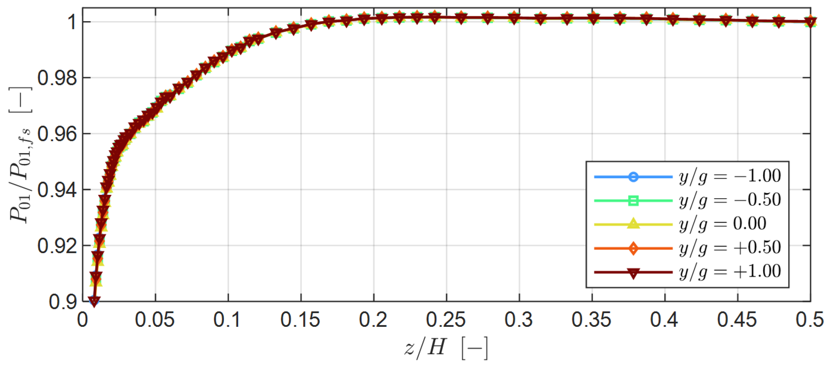
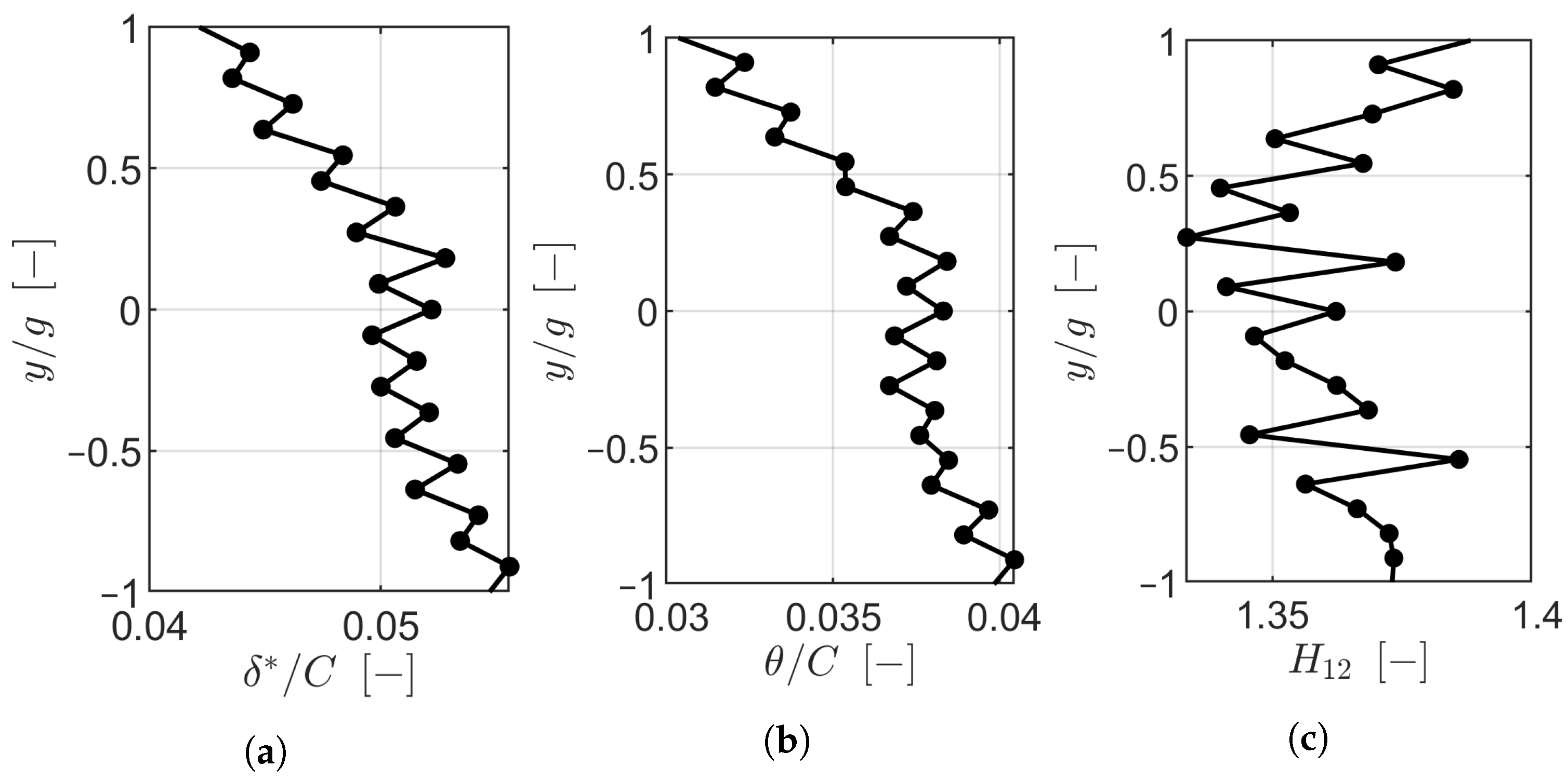
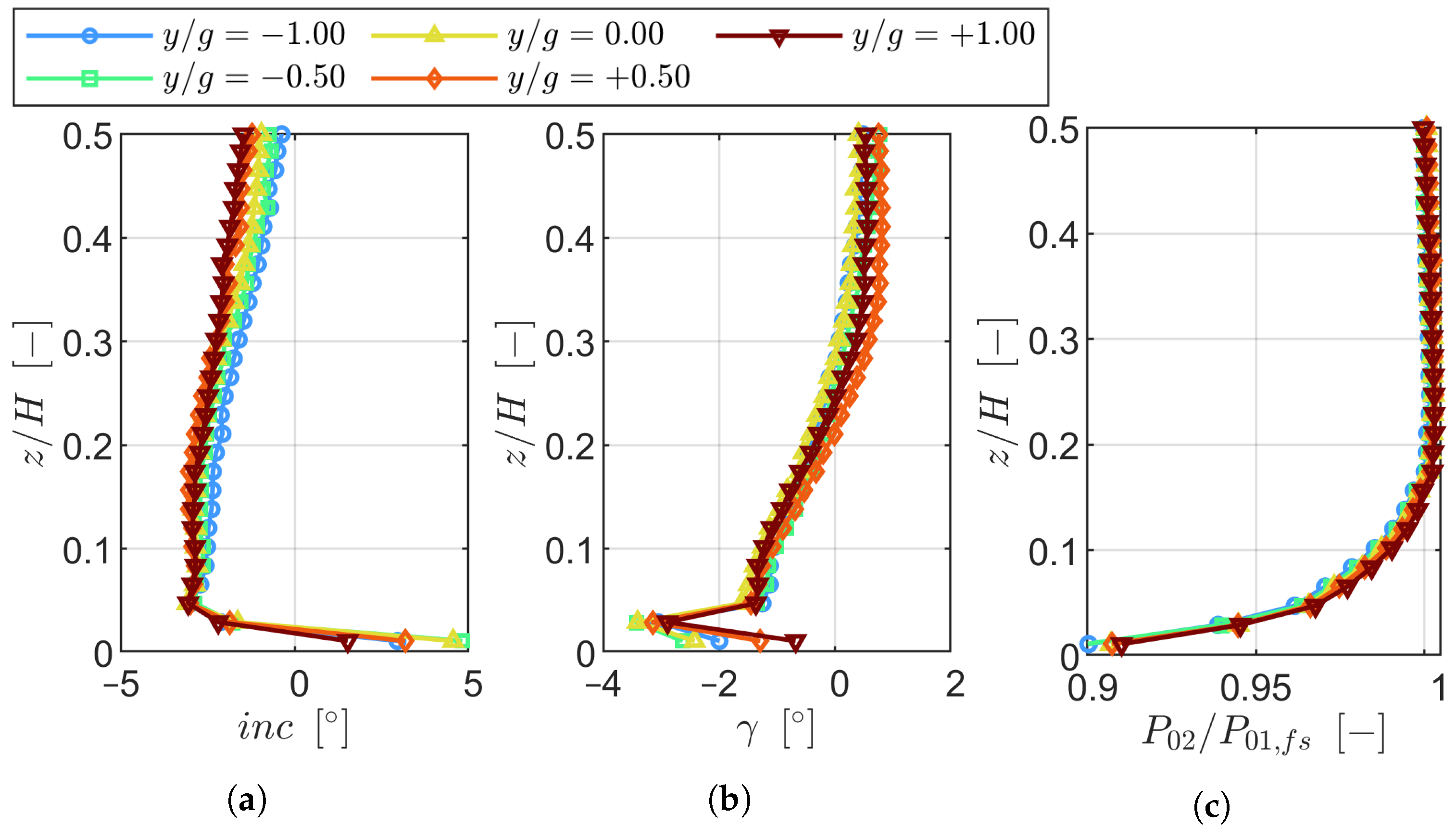
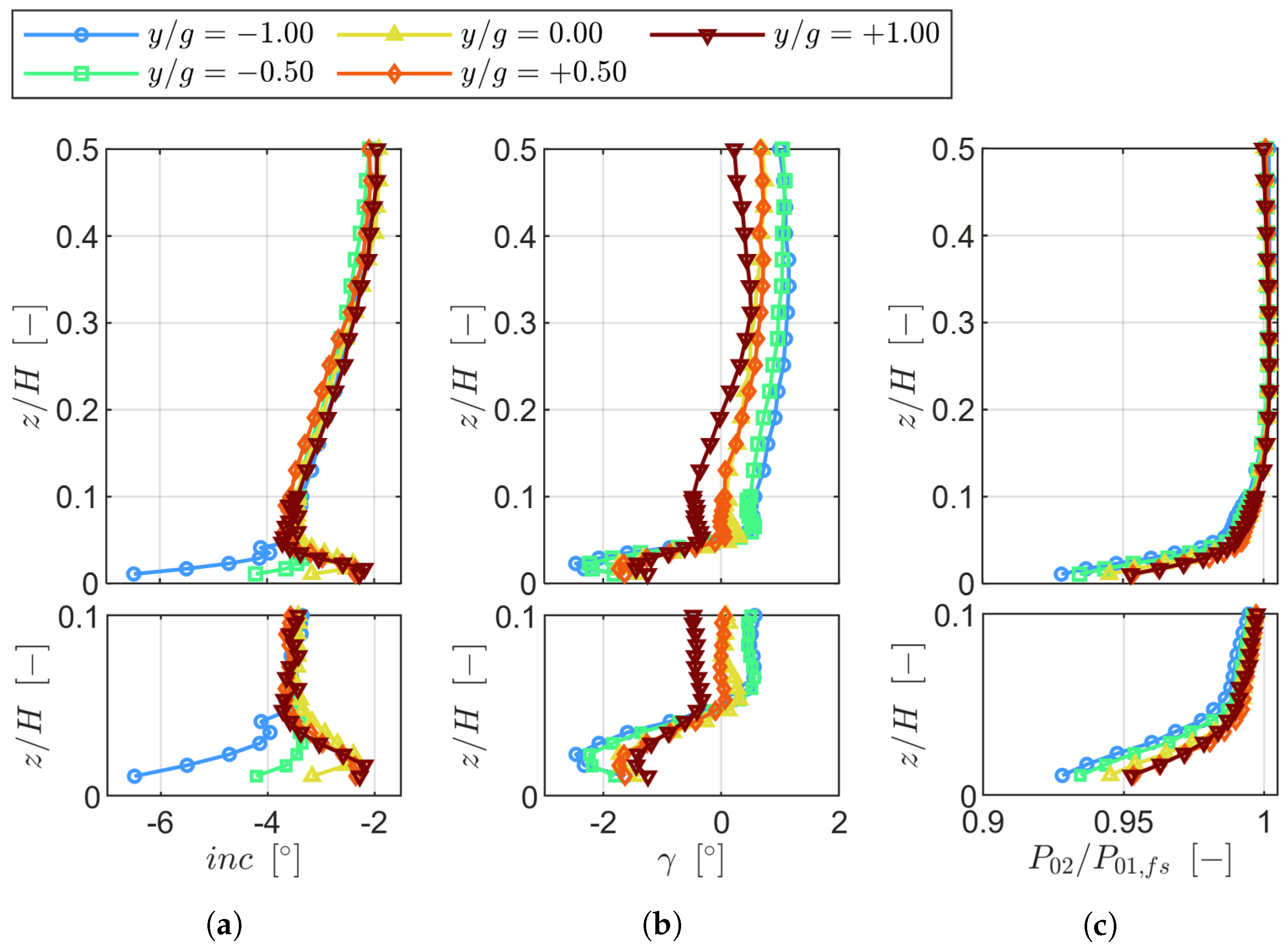
The periodicity of the inlet boundary layer at Plane 01 was characterized by low variability, with displacement thickness variations within ±0.35% of the chord and total pressure deviations below 0.10%. However, nonuniformities emerged downstream at Plane 02 due to the wake generator, in particular near the endwall, where the incidence varied by up to ±2.00$°$ and the total pressure by ±1.25%. These variations were linked to boundary layer thickness growth and skewness, which contributed to localized flow nonperiodicity.

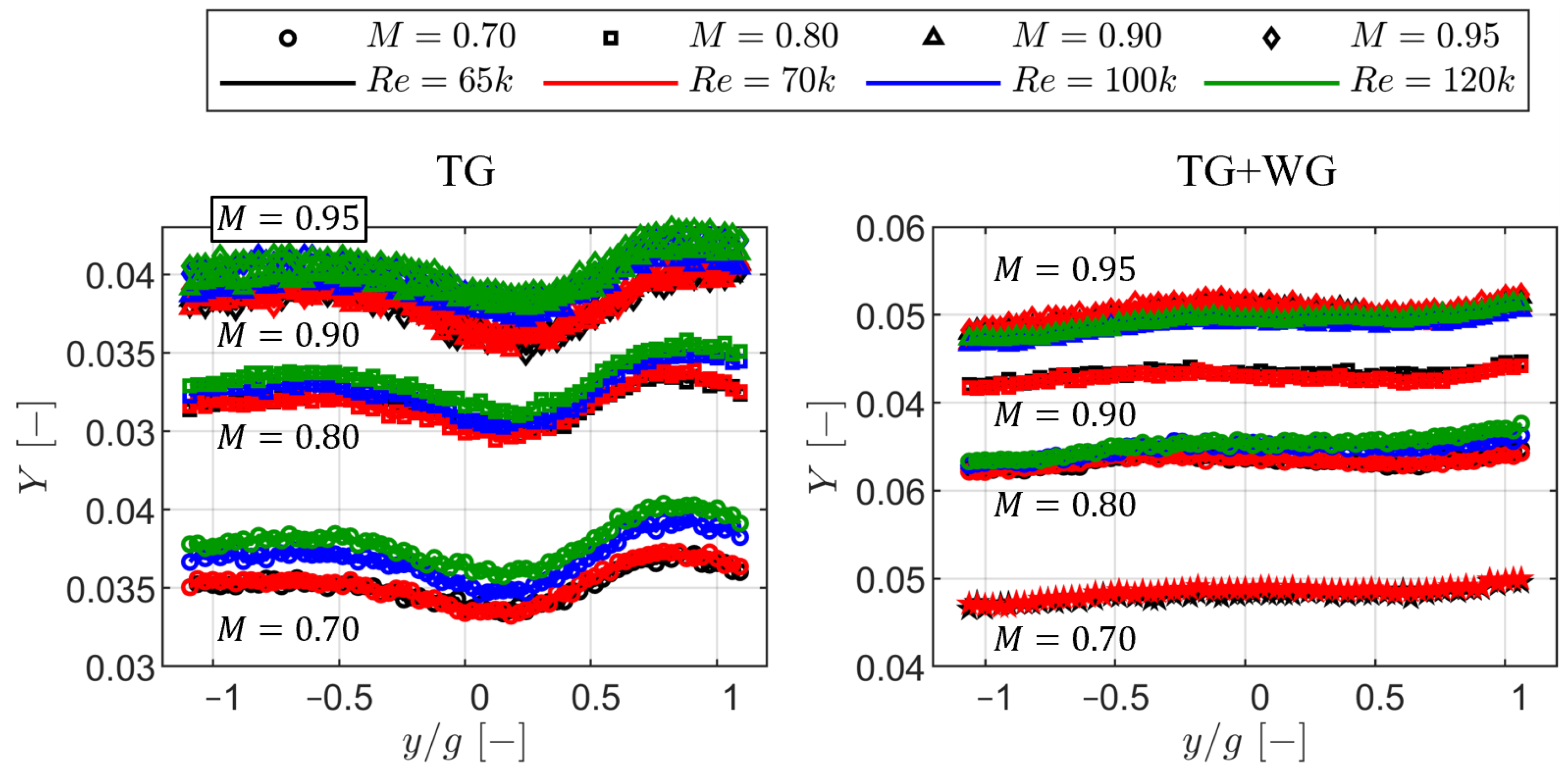
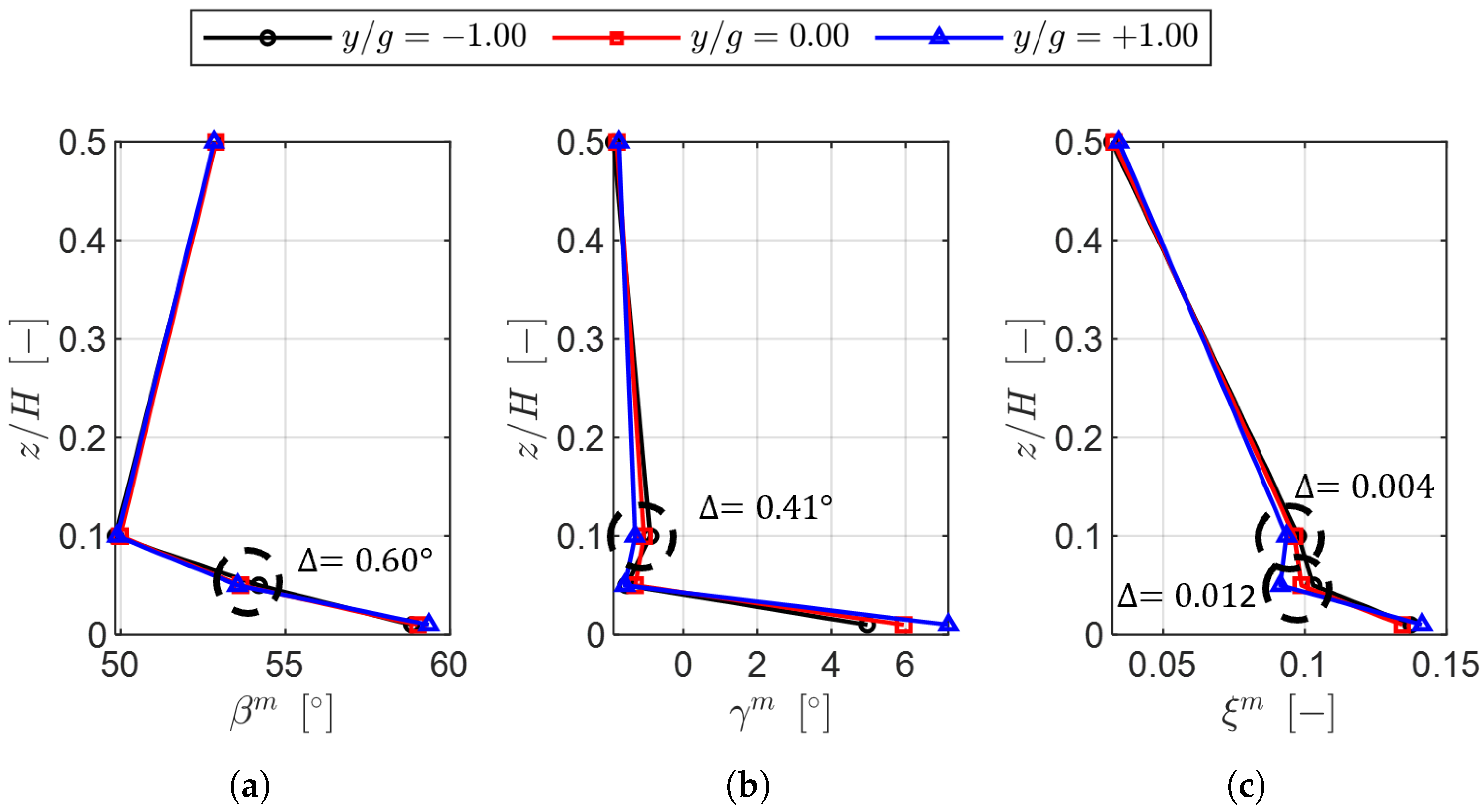
At the cascade outlet, the wake generator amplified pitch-to-pitch variations in the kinetic energy loss coefficient, with maximum deviations reaching ±0.5% in the secondary flow region. The increased inlet boundary layer thickness and negative skewness toward negative pitchwise locations correlated with higher secondary losses, as predicted by the Coull and Clark model [23], resulting in a secondary loss increase of approximately 0.014. The introduction of purge flow significantly mitigated these periodicity variations, particularly near the endwall, which was due to stabilizing of the secondary flow structures and reducing the displacement of the loss cores.

This work constitutes the baseline for a thorough investigation of the impact of unsteady wakes on the combined interaction of secondary flows and purge flows in high-speed low-pressure turbine geometries operating at engine-relevant conditions.

References

1. IEA. CO2 Emissions in 2022; IEA: Paris, France, 2023. [Google Scholar]
2. European Commission, Directorate-General for Research and Innovation. Fly the Green Deal–Europe’s Vision for Sustainable Aviation; Publications Office of the European Union: Luxembourg, 2022. Available online: https://op.europa.eu/en/publication-detail/-/publication/69dfdaf4-07d5-11ed-acce-01aa75ed71a1/language-en (accessed on 5 January 2025).
3. Air Transport Action Group. Waypoint 2050: Balancing Growth in Connectivity with a Comprehensive Global Air Transport Response to the Climate Emergency: A Vision of Net-Zero Aviation by Mid-Century; Air Transport Action Group: Geneva, Switzerland, 2021. [Google Scholar]
4. Kurzke, J. Fundamental Differences Between Conventional and Geared Turbofans. In Proceedings of the ASME Turbo Expo 2009: Power for Land, Sea, and Air, Orlando, FL, USA, 8–12 June 2009; Volume 48821, pp. 145–153. [Google Scholar] [CrossRef]
5. Lu, W.; Huang, G.; Xiang, X.; Wang, J.; Yang, Y. Thermodynamic and Aerodynamic Analysis of an Air-Driven Fan System in Low-Cost High-Bypass-Ratio Turbofan Engine. Energies 2019, 12, 1917. [Google Scholar] [CrossRef]
6. Stankowski, T.; MacManus, D.; Robinson, M.; Sheaf, C. Aerodynamic Effects of Propulsion Integration for High Bypass Ratio Engines. J. Aircr. 2017, 54, 2270–2284. [Google Scholar] [CrossRef]
7. Hughes, C.; Van Zante, D.; Heidmann, J. Aircraft engine technology for green aviation to reduce fuel burn. In Proceedings of the 3rd AIAA Atmospheric Space Environments Conference, Honolulu, HI, USA, 27–30 June 2011; p. 3531. [Google Scholar]
8. Smith, S. A Simple Correlation of Turbine Efficiency. Aeronaut. J. 1965, 69, 467–470. [Google Scholar] [CrossRef]
9. Bernardini, C.; Benton, S.I.; Lee, J.D.; Bons, J.P.; Chen, J.P.; Martelli, F. Steady Vortex-Generator Jet Flow Control on a Highly Loaded Transonic Low-Pressure Turbine Cascade: Effects of Compressibility and Roughness. J. Turbomach. 2014, 136, 111003. [Google Scholar] [CrossRef]
10. Giovannini, M.; Rubechini, F.; Marconcini, M.; Arnone, A.; Bertini, F. Analysis of a LPT Rotor Blade for a Geared Engine: Part I—Aero-Mechanical Design and Validation. In Proceedings of the ASME Turbo Expo 2016: Turbomachinery Technical Conference and Exposition, Seoul, Republic of Korea, 13–17 June 2016; p. V02BT38A053. [Google Scholar] [CrossRef]
11. Malzacher, F.; Gier, J.; Lippl, F. Aerodesign and Testing of an Aeromechanically Highly Loaded LP Turbine. J. Turbomach. 2003, 128, 643–649. [Google Scholar] [CrossRef]
12. Torre, D.; GarcIa-Valdecasas, G.; Puente, A.; HernAndez, D.; Luque, S. Design and Testing of a Multi-Stage Intermediate Pressure Turbine for Future Geared Turbofans. J. Turbomach. 2022, 144, 091008. [Google Scholar] [CrossRef]
13. Howell, R.J.; Ramesh, O.N.; Hodson, H.P.; Harvey, N.W.; Schulte, V. High Lift and Aft-Loaded Profiles for Low-Pressure Turbines. J. Turbomach. 2000, 123, 181–188. [Google Scholar] [CrossRef]
14. Hodson, H.P.; Howell, R.J. The role of transition in high-lift low-pressure turbines for aeroengines. Prog. Aerosp. Sci. 2005, 41, 419–454. [Google Scholar] [CrossRef]
15. Stieger, R.D.; Hodson, H.P. The Unsteady Development of a Turbulent Wake Through a Downstream Low-Pressure Turbine Blade Passage. J. Turbomach. 2005, 127, 388–394. [Google Scholar] [CrossRef]
16. Coton, T.; Arts, T.; Lefebvre, M.; Liamis, N. Unsteady and Calming Effects Investigation on a Very High-Lift LP Turbine Blade—Part I: Experimental Analysis. J. Turbomach. 2003, 125, 281–290. [Google Scholar] [CrossRef]
17. Vázquez, R.; Torre, D. The Effect of Mach Number on the Loss Generation of LP Turbines. In Proceedings of the ASME Turbo Expo 2012: Turbine Technical Conference and Exposition, Copenhagen, Denmark, 11–15 June 2012; pp. 1131–1142. [Google Scholar] [CrossRef]
18. Börner, M.; Niehuis, R. Dynamics of Shock Waves Interacting with Laminar Separated Transonic Turbine Flow Investigated by High-Speed Schlieren and Surface Hot-Film Sensors. J. Turbomach. 2021, 143, 051010. [Google Scholar] [CrossRef]
19. Vera, M.; Hodson, H.P.; Vazquez, R. The Effects of a Trip Wire and Unsteadiness on a High-Speed Highly Loaded Low-Pressure Turbine Blade. J. Turbomach. 2004, 127, 747–754. [Google Scholar] [CrossRef]
20. Vera, M.; Hodson, H.; Vazquez, R. The Effect of Mach Number on LP Turbine Wake-Blade Interaction. In Proceedings of the Unsteady Aerodynamics, Aeroacoustics and Aeroelasticity of Turbomachines; Hall, K.C., Kielb, R.E., Thomas, J.P., Eds.; Springer: Dordrecht, The Netherlands, 2006; pp. 203–216. [Google Scholar]
21. Vázquez, R.; Antoranz, A.; Cadrecha, D.; Armananzas, L. The Influence of Reynolds Number, Mach Number and Incidence Effects on Loss Production in Low Pressure Turbine Airfoils. In Proceedings of the ASME Turbo Expo 2006: Power for Land, Sea, and Air, Barcelona, Spain, 8–11 May 2006; pp. 949–960. [Google Scholar] [CrossRef]
22. Coull, J.D. Endwall Loss in Turbine Cascades. J. Turbomach. 2017, 139, 081004. [Google Scholar] [CrossRef]
23. Coull, J.D.; Clark, C.J. The Effect of Inlet Conditions on Turbine Endwall Loss. J. Turbomach. 2022, 144, 101011. [Google Scholar] [CrossRef]
24. Simoni, D.; Berrino, M.; Ubaldi, M.; Zunino, P.; Bertini, F. Off-Design Performance of a Highly Loaded Low Pressure Turbine Cascade Under Steady and Unsteady Incoming Flow Conditions. J. Turbomach. 2015, 137, 071009. [Google Scholar] [CrossRef]
25. Giovannini, M.; Rubechini, F.; Marconcini, M.; Simoni, D.; Yepmo, V.; Bertini, F. Secondary Flows in LPT Cascades: Numerical and Experimental Investigation of the Impact of the Inner Part of the Boundary Layer. In Proceedings of the ASME Turbo Expo 2018: Turbomachinery Technical Conference and Exposition, Oslo, Norway, 11–15 June 2018; p. V02BT41A027. [Google Scholar] [CrossRef]
26. Schubert, T.; Chemnitz, S.; Niehuis, R. The Effects of Inlet Boundary Layer Condition and Periodically Incoming Wakes on Secondary Flow in a Low Pressure Turbine Cascade. J. Turbomach. 2021, 143, 041001. [Google Scholar] [CrossRef]
27. Simonassi, L.; Lopes, G.; Gendebien, S.; Torre, A.F.M.; Patinios, M.; Lavagnoli, S.; Zeller, N.; Pintat, L. An Experimental Test Case for Transonic Low-Pressure Turbines—Part I: Rig Design, Instrumentation and Experimental Methodology. In Proceedings of the ASME Turbo Expo 2022: Turbomachinery Technical Conference and Exposition, Rotterdam, The Netherlands, 13–17 June 2022; p. V10BT30A012. [Google Scholar] [CrossRef]
28. Arts, T. Aerodynamic performance of two very high lift low pressure turbine airfoils (T106C–T2) at low Reynolds and high Mach numbers. In Proceedings of the 5th European Conference for Aerospace Sciences, Munich, Germany, 1–5 July 2013. [Google Scholar]
29. Clinckemaillie, J.; Fattorini, L.; Fontani, T.; Nuyts, C.; Wain, G.; Arts, T. Aerodynamic performance of a very-high-lift low-pressure turbine airfoil (T106C) at low Reynolds and high Mach number including the effect of incoming periodic wakes. In Proceedings of the 11th European Conference on Turbomachinery Fluid Dynamics and Thermodynamics, ETC 2015, Madrid, Spain, 23–27 March 2015. [Google Scholar]
30. Lopes, G.; Simonassi, L.; Lavagnoli, S. Time-Averaged Aerodynamics of a High-Speed Low-Pressure Turbine Cascade with Cavity Purge and Unsteady Wakes. J. Turbomach. 2023, 146, 021008. [Google Scholar] [CrossRef]
31. Lopes, G.; Simonassi, L.; Lavagnoli, S. Impact of Unsteady Wakes on the Secondary Flows of a High-Speed Low-Pressure Turbine Cascade. Int. J. Turbomach. Propuls. Power 2023, 8, 36. [Google Scholar] [CrossRef]
32. Simonassi, L.; Lopes, G.; Lavagnoli, S. Effects of Periodic Incoming Wakes on the Aerodynamics of a High-Speed Low-Pressure Turbine Cascade. Int. J. Turbomach. Propuls Power 2023, 8, 35. [Google Scholar] [CrossRef]
33. Brear, M.J.; Hodson, H.P.; Gonzalez, P.; Harvey, N.W. Pressure Surface Separations in Low-Pressure Turbines—Part 2: Interactions with the Secondary Flow. J. Turbomach. 2002, 124, 402–409. [Google Scholar] [CrossRef]
34. Melzer, A.P.; Pullan, G. The Role of Vortex Shedding in the Trailing Edge Loss of Transonic Turbine Blades. J. Turbomach. 2019, 141, 041001. [Google Scholar] [CrossRef]
35. Menter, F.R. Two-equation eddy-viscosity turbulence models for engineering applications. AIAA J. 1994, 32, 1598–1605. [Google Scholar] [CrossRef]
36. Lopes, G. Aerodynamics of a High-Speed Low-Pressure Turbine Cascade with Unsteady Wakes and Purge Flow. Ph.D. Thesis, Université de Liège, Liège, Belgium, 2024. [Google Scholar] [CrossRef]
37. Coull, J.D.; Hodson, H.P. Blade Loading and Its Application in the Mean-Line Design of Low Pressure Turbines. J. Turbomach. 2012, 135, 021032. [Google Scholar] [CrossRef]
38. Hourmouziadis, J. Aerodynamic Design of Low Pressure Turbines. In Blading Design for Axial Turbomachines; AGARD Lecture Series No. 167, Paper 8; Advisory Group for Aerospace Research and Development: Neuilly-sur-Seine, France, June 1989. [Google Scholar]
39. Hanson, R.E.; Buckley, H.P.; Lavoie, P. Aerodynamic optimization of the flat-plate leading edge for experimental studies of laminar and transitional boundary layers. Exp. Fluids 2012, 53, 863–871. [Google Scholar] [CrossRef]
40. Roach, P. The generation of nearly isotropic turbulence by means of grids. Int. J. Heat Fluid Flow 1987, 8, 82–92. [Google Scholar] [CrossRef]
41. Pfeil, H.; Herbst, R.; Schröder, T. Investigation of the Laminar-Turbulent Transition of Boundary Layers Disturbed by Wakes. J. Eng. Power 1983, 105, 130–137. [Google Scholar] [CrossRef]
42. Lopes, G.; Simonassi, L.; Torre, A.; Lavagnoli, S. Instrumentation Interference in a Transonic Linear Cascade. J. Phys. Conf. Ser. 2023, 2511, 012018. [Google Scholar] [CrossRef]
43. Torre, A.F.M.; Patinios, M.; Lopes, G.; Simonassi, L.; Lavagnoli, S. Vane–Probe Interactions in Transonic Flows. J. Turbomach. 2023, 145, 061010. [Google Scholar] [CrossRef]
44. Gracey, W.; Letko, W.; Russell, W. Wind-Tunnel Investigation of a Number of Total-Pressure Tubes at High Angles of Attack Subsonic Speeds; Technical Report; National Aeronautics and Space Administration Hampton va Langley Research Center: Hampton, VA, USA, 1951. [Google Scholar]
45. Barker, M. On the use of very small pitot-tubes for measuring wind velocity. In Proceedings of the Royal Society of London. Series A, Containing Papers of a Mathematical and Physical Character; The Royal Society: London, UK, 1922; Volume 101, pp. 435–445. [Google Scholar]
46. MacMillan, F. Experiments on Pitot-Tubes in Shear Flow; Cambridge University Press: Cambridge, UK, 1956. [Google Scholar]
47. Pastorino, G.; Simonassi, L.; Lopes, G.; Boufidi, E.; Fontaneto, F.; Lavagnoli, S. Measurements of Turbulence in Compressible Low-Density Flows at the Inlet of a Transonic Linear Cascade with and without Unsteady Wakes. J. Turbomach. 2024, 146, 071002. [Google Scholar] [CrossRef]
48. Treaster, A.; Yocum, A. The Calibration and Application of Five-Hole Probes; Technical Report; Pennsylvania State Univ University Park Applied Research Lab: State College, PA, USA, 1978. [Google Scholar]
49. Yasa, T.; Paniagua, G. Robust procedure for multi-hole probe data processing. Flow Meas. Instrum. 2012, 26, 46–54. [Google Scholar] [CrossRef]
50. Passmann, M.; der Wiesche, S.a.; Povey, T.; Bergmann, D. Effect of Reynolds Number on Five-Hole Probe Performance: Experimental Study of the Open-Access Oxford Probe. J. Turbomach. 2021, 143, 091003. [Google Scholar] [CrossRef]
51. Bohn, D. Untersuchung Zweier Verschiedener Axialer Überschallverdichterstufen unter Besonderer Berücksichtigung der Wechselwirkungen Zwischen Luft-und Leitrad; Technical Report; Institute for Jet Propulsion and Turbomachinery, RWTH Aachen University: Aachen, Germany, 1977. [Google Scholar]
52. Lenherr, C.; Kalfas, A.; Abhari, R. High temperature fast response aerodynamic probe. J. Eng. Gas Turbines Power 2011, 133, 011603. [Google Scholar] [CrossRef]
53. Bosdas, I.; Mansour, M.; Kalfas, A.I.; Abhari, R.S.; Senoo, S. Unsteady Wet Steam Flow Field Measurements in the Last Stage of Low Pressure Steam Turbine. J. Eng. Gas Turbines Power 2015, 138, 032601. [Google Scholar] [CrossRef]
54. Brouckaert, J. Development of Fast Response Aerodynamic Pressure Probes for Time-Resolved Measurements in Turbomachines: Thesis Presented in Order to Obtain the Degree of Docteur en Sciences Appliquées, Université Libre de Bruxelles, October 2002; Von Karman Institute for Fluid Dynamics: Sint-Genesius-Rode, Belgium, 2004. [Google Scholar]
55. Bergh, H.; Tijdeman, H. Theoretical and Experimental Results for the Dynamic Response of Pressure Measuring Systems; Technical Report; National Aerospace Laboratory (NLR): Amsterdam, The Netherlands, 1965. [Google Scholar]
56. Pfau, A.; Schlienger, J.; Kalfas, A.I.; Abhari, R. Virtual four sensor fast response aerodynamic probe (FRAP®). In E3S Web of Conferences; EDP Sciences: Paris, France, 2022; Volume 345, p. 01014. [Google Scholar]
57. Gaetani, P.; Persico, G. Technology Development of Fast-Response Aerodynamic Pressure Probes. Int. J. Turbomach. Propuls. Power 2020, 5, 6. [Google Scholar] [CrossRef]
58. Hougen, J.; Martin, O.; Walsh, R. Dynamics of pneumatic transmission lines. Control Eng. 1963, 10, 114–117. [Google Scholar]
59. Vera, M.; de la Rosa Blanco, E.; Hodson, H.; Vazquez, R. Endwall Boundary Layer Development in an Engine Representative Four-Stage Low Pressure Turbine Rig. J. Turbomach. 2008, 131, 011017. [Google Scholar] [CrossRef]
60. Abernethy, R.; Benedict, R.; Dowdell, R. ASME Measurement Uncertainty. J. Fluids Eng. 1985, 107, 161–164. [Google Scholar] [CrossRef]
61. Coleman, H.; Steele, W. Experimentation, Validation, and Uncertainty Analysis for Engineers; John Wiley & Sons: Hoboken, NJ, USA, 2018. [Google Scholar]
62. Michálek, J.; Monaldi, M.; Arts, T. Aerodynamic Performance of a Very High Lift Low Pressure Turbine Airfoil (T106C) at Low Reynolds and High Mach Number with Effect of Free Stream Turbulence Intensity. J. Turbomach. 2012, 134, 061009. [Google Scholar] [CrossRef]
63. Schlichting, H.; Gersten, K. Boundary-Layer Theory; Springer: Berlin/Heidelberg, Germany, 2016. [Google Scholar]
64. Walsh, J.A.; Gregory-Smith, D.G. Inlet Skew and the Growth of Secondary Losses and Vorticity in a Turbine Cascade. J. Turbomach. 1990, 112, 633–642. [Google Scholar] [CrossRef]
Figure 1. Schematic view of 1.5 low-pressure turbine stages and linearly extruded region of interest.
Ijtpp 10 00002 g001
Figure 2. The VKI S-1/C wind tunnel.
Ijtpp 10 00002 g002
Figure 3. The SPLEEN C1 geometry (a) and blade loading at design point (b).
Ijtpp 10 00002 g003
Figure 4. Cascade mounted in VKI S-1/C wind tunnel highlighting boundary layer lip and turbulence grid.
Ijtpp 10 00002 g004
Figure 5. The SPLEEN cascade test section setup (a), and test section equipped with WG bars and cavity slot (b).
Ijtpp 10 00002 g005
Figure 6. Blade-to-blade view of the cascade highlighting the measurements planes.
Ijtpp 10 00002 g006
Figure 7. Meridional view of linear cascade test section highlighting the distribution of instrumentation.
Ijtpp 10 00002 g007
Figure 8. Aerodynamic probes used throughout the experimental campaign.
Ijtpp 10 00002 g008
Figure 9. Sketch of the V4HP probe highlighting the accommodation of sensors in the probe head and the resulting line–cavity system.
Ijtpp 10 00002 g009
Figure 10. Location and dimensions of the instrumentation on the blade surface, showing the blade traversing unit and SS instrumented sliding blade.
Ijtpp 10 00002 g010
Figure 11. Endwall inserts: Pneumatic and FR pressure tap Insert 1 (left top) and Insert 2 (left bottom) and location of the taps in the passage by combining the instrumentation of both inserts in one passage (right).
Ijtpp 10 00002 g011
Figure 12. Pitchwise distribution of turbulent quantities in the absence of wake generator: turbulence intensity (a) and integral length scale (b).
Ijtpp 10 00002 g012
Figure 13. Radial profiles of turbulence: turbulence intensity (a) and integral length scale (b).
Ijtpp 10 00002 g013
Figure 14. Pitchwise distribution of total loss coefficient for the different investigated flow conditions.
Ijtpp 10 00002 g014
Figure 15. Turbulence grid loss coefficient correlation as a function of inlet and outlet flow conditions for the case with TG only.
Ijtpp 10 00002 g015
Figure 16. Spanwise distribution of normalized total pressure at Plane 01.
Ijtpp 10 00002 g016
Figure 17. Pitchwise distribution of BL integral parameters measured at Plane 01: displacement thickness (a), momentum thickness (b), and shape factor (c). The true chord normalizes the displacement and momentum thickness.
Ijtpp 10 00002 g017
Figure 18. Spanwise distributions at Plane 02 during the first phase of testing: inlet flow incidence (a), cascade pitch angle (b), and normalized total pressure (c).
Ijtpp 10 00002 g018
Figure 19. Spanwise distributions at Plane 02 during the second phase of testing: inlet flow incidence (a), cascade pitch angle (b), and normalized total pressure (c).
Ijtpp 10 00002 g019
Figure 20. Pitchwise mass-averaged profiles obtained for different wakes downstream of the cascade: primary flow direction (a), cascade pitch angle (b), and kinetic energy loss coefficient (c).
Ijtpp 10 00002 g020
Figure 21. Re-shifted pitchwise distribution of kinetic energy loss coefficient measured during the first phase: z/H = 0.05 (a), z/H = 0.10 (b), and z/H = 0.50 (c).
Ijtpp 10 00002 g021
Figure 22. Periodicity of the cascade outlet flow field for the second testing phase: primary flow direction (a) and kinetic energy loss coefficient (b).
Ijtpp 10 00002 g022
Figure 23. Pitchwise mass-averaged profiles obtained for different wakes downstream of the cascade during the second phase: primary flow direction (a), cascade pitch angle (b), and kinetic energy loss coefficient (c).
Ijtpp 10 00002 g023
Figure 24. Re-shifted pitchwise distribution of the loss coefficient at z/H = 0.50 measured during the second phase.
Ijtpp 10 00002 g024
Figure 25. Periodicity of the cascade outlet flow field with wake generator and purge flow: primary flow direction (a) and kinetic energy loss coefficient (b).
Ijtpp 10 00002 g025
Figure 26. Pitchwise mass-averaged profiles obtained for different wakes downstream of the cascade during the third phase: primary flow direction (a), cascade pitch angle (b), and kinetic energy loss coefficient (c).
Ijtpp 10 00002 g026