Aerial Remote Sensing and Urban Planning Study of Ancient Hippodamian System

Abstract

In ancient Olynthus (Greece), an Unmanned Aircraft System (UAS) was utilized to collect both RGB and multispectral (MS) images of the archaeological site. Ground Control Points (GCPs) were used to solve the blocks of images and the production of Digital Surface Models (DSMs) and orthophotomosaics. Check Points (CPs) were employed to verify the spatial accuracy of the products. The innovative image fusion process carried out in this paper, which combined the RGB and MS orthophotomosaics from UAS sensors, led to the creation of a fused image with the best possible spatial resolution (five times better than that of the MS orthophotomosaic). This improvement facilitates the optimal visual and digital (e.g., classification) analysis of the archaeological site. Utilizing the fused image and reviewing the literature, the paper compiles and briefly presents information on the Hippodamian system of the excavated part of the ancient city of Olynthus (regularity, main and secondary streets, organization of building blocks, public and private buildings, types and sizes of dwellings, and internal organization of buildings) as well as information on its socio-economic organization (different social groups based on the characteristics of the buildings, commercial markets, etc.).

1. Introduction

Mapping an archaeological site today can be accomplished using high spatial resolution and accuracy equipment, such as laser scanners, Unmanned Aircraft Systems (UAS), etc. The products generated (Digital Surface Models and/or orthophotomosaics) contain rich thematic information. To create and/or validate these products, it is essential to use additional high spatial accuracy instruments in the field, such as Global Navigation Satellite System (GNSS) receivers [1,2,3,4].

In the case of UAS, the thematic information (completeness, resolution, and overall quality of the objects) of the images varies depending on the sensor used. An RGB sensor will capture objects in the visible spectrum with a spatial resolution of a few millimeters from a low flight altitude, whereas a multispectral (MS) sensor, operating from the same altitude, captures objects in spectral bands beyond the visible with a spatial resolution of a few centimeters. For example, the UAS Phantom 4 collects RGB images (using its 1/2.3” CMOS 12.4 Mp RGB sensor) at an approximate spatial resolution of 1.5 cm from a flight height of 40 m, while it gathers MS images (using the Sequoia+ MS sensor by Parrot 1.2 Mp (Parrot SA, Paris, France), covering green, red, Red Edge, and near infrared (NIR) bands) at about 4 cm resolution from the same height [5]. The UAS Wingtra GEN II (Wingtra AG, Zurich, Switzerland) collects RGB images (using the Sony RX1R II 42.4 Mp RGB sensor, Sony Group Corporation, Tokyo, Japan) with a spatial resolution of 1.5 cm from a flight height of 100 m, and from that same height, it acquires MS images (using the MicaSense RedEdge-MX 1.2 Mp MS sensor, covering blue, green, red, Red Edge, and NIR, MicaSense Inc., Seattle, United States) at a resolution of approximately 7 cm [6]. Thus, while the spatial resolution of the thematic information in RGB images is excellent, the corresponding resolution of MS images is not acceptable for archaeologists when they require orthophotomosaics at scales of 1:50 or 1:100.

This is why the first author since 2020 conducted original research on image fusion [5,6,7], utilizing the RGB and MS images from the UAS sensors. The ultimate goal is to produce a fused image that retains the spectral information of the original MS image while achieving the spatial solution of the RGB image, thereby enhancing the spatial resolution of the thematic data contained in the MS image.

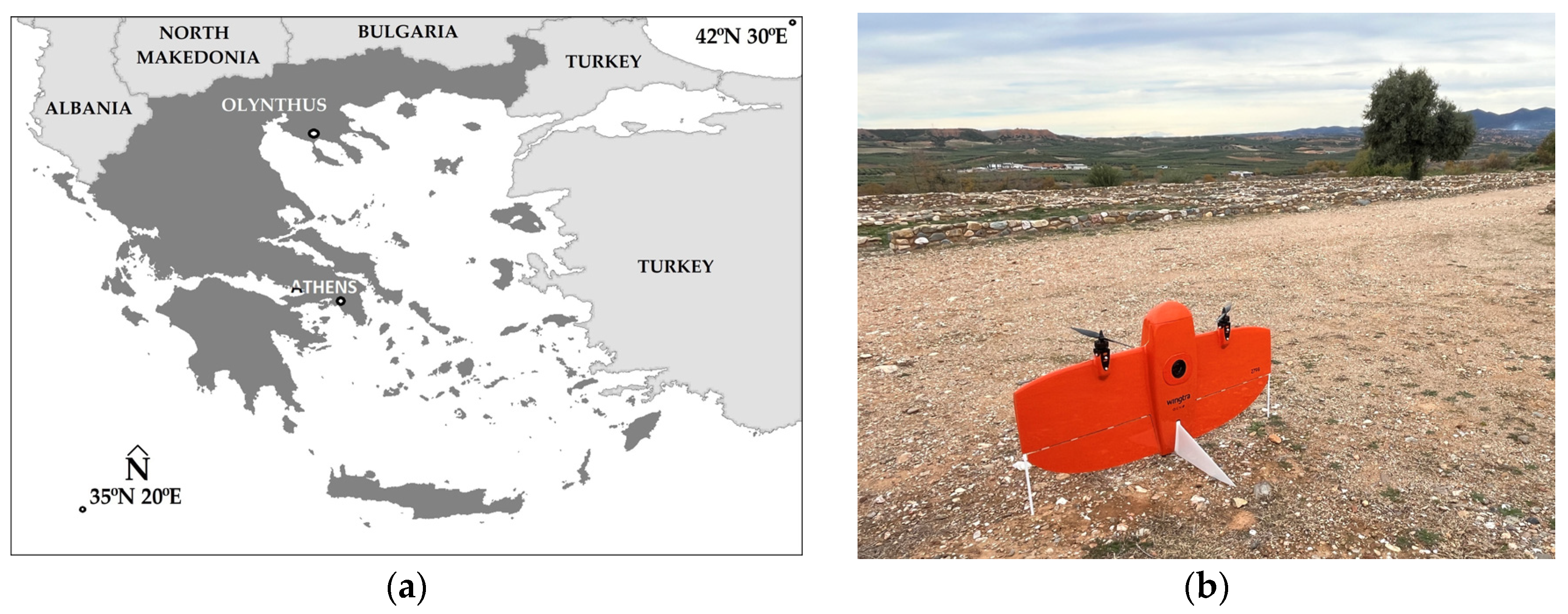
In this study, the UAS Wingtra GEN II (Wingtra AG, Zurich, Switzerland) was used to collect RGB and MS images of the Hippodamian system of ancient Olynthus (Central Macedonia, Greece, Figure 1). Ground Control Points (GCPs) were measured in the field using GNSS to solve the blocks of images and produce Digital Surface Models (DSMs) and orthophotomosaics. Corresponding products were also generated using the UAS’s Post-processed Kinematic (PPK) system (without the use of GCPs). Check Points (CPs) were measured in the field for quantitative control of products, which is the first objective of the study (to assess the horizontal and vertical accuracy of the products). The primary methods for evaluating a product include calculating the mean, standard deviation, and Root Mean Square Error (RMSE) [8,9,10,11]. Additionally, when the data follow a normal distribution, analysis of variance (ANOVA) is used for hypothesis testing. This process helps identify differences in mean values and standard deviations across various datasets, such as the measurements on the products versus those taken in the field [6].

The second objective of the study is to perform image fusion using the RGB and MS images and to validate the resulting fused image. The proposed process is innovative and was initiated by the first author as early as 2020. It is expected that the findings of this study will, once again, confirm the effectiveness of the proposed image fusion process, utilizing the RGB and MS images from the UAS sensors. Finally, by studying the products (and the new fused image with the multispectral information of the original MS, but with much better spatial resolution than the original MS, thus increasing the capacity for the visual observation and interpretation of objects) and reviewing the literature, the third objective is to investigate and present information about the Hippodamian system of ancient Olynthus. This includes details on urban planning and architectural structures (regularity, main and secondary streets, organization of building blocks, hydraulic works, public and private buildings, types and sizes of dwellings, and the internal organization of buildings) as well as information on its socio-economic organization (different social groups based on the characteristics of the buildings, commercial markets, etc.).

2. Study Area

Ancient Olynthus (Central Macedonia, Greece, 40°17′47.52″ N 23°21′15.37″ E) was one of the most important cities of antiquity. According to Herodotus, it was founded (around the mid-7th century BC) by the Bottiaeans (ancient Greeks originally inhabiting Western and after Central Macedonia), who, after being expelled by the Macedonians, resettled in Chalkidiki. The city was destroyed in 479 BC by the Persians as they returned to Asia following their defeat at Plataea. Its period of prosperity dates back to the Classical era. From 440 BC to 420 BC, it became the most populous and wealthy city in the region, built according to the Hippodamian system. Due to its growing power, it endured successive attacks for an extended period, until Philip II ultimately destroyed it in 348 BC [12].

Systematic archaeological excavations began during the interwar period by the American School of Classical Studies. To date, part of the city has been studied, revealing one of the best-preserved examples of urban planning, the Hippodamian system, and the exceptional residential architecture of the Classical era. The city is renowned for the well-preserved mosaic floors of its private buildings, which depict mythological scenes and geometric patterns. Additionally, there were public buildings, temples, and marketplaces. Finally, underground water tanks and drainage systems have been discovered, indicative of the advanced engineering of the period. Ancient Olynthus provides one of the best surviving images of ancient Greek urban planning [12].

3. Equipment

To capture aerial imagery at the ancient Olynthus, the UAS WingtraOne GEN II (Wingtra AG, Zurich, Switzerland) (Figure 1), a vertical takeoff and landing (VTOL) fixed-wing UAS (weight 3.7 kg and dimensions 125 × 68 × 12 cm³), was used. It has a maximum flight duration of 59 min. To determine the coordinates of the captured image centers, it employs an integrated multi-frequency PPK GNSS antenna, compatible with GPS (L1 and, L2), GLONASS (L1 and L2), Galileo (L1), and BeiDou (L1). The flight plan and parameters are configured using the WingtraPilot© v2.17.0 software. Additionally, the system is equipped with an RGB and MS sensor. Sony RX1R II (Sony Group Corporation, Tokyo, Japan) is a full-frame RGB sensor with a 35 mm focal length and a resolution of 42.4 Mp. It also provides images with a spatial resolution of 1.6 cm/pixel at a flight height of 120 m. The MicaSense RedEdge-MX (MicaSense Inc., Seattle, United States) is a MS sensor with a 5.5 mm focal length and 1.2 Mp resolution, including having five spectral bands, blue, green, red, Red Edge and NIR, and a spatial resolution of 8.2 cm/pixel at a flight height of 120 m [13,14].

The Topcon HiPer SR GNSS receiver (Topcon Positioning Systems, Tokyo, Japan) was used for two reasons. The first was to measure the GCPs and CPs with real-time kinematic (RTK) positioning before the flights, and the second was to collect the necessary measurements using the static method during the flights, which will allow for the calculation of the coordinates of the image centers. This system supports multiple satellite signals, including GPS (L1, L2, and L2C), GLONASS (L1, L2, and 2C), and SBAS-QZAA (L1 and L2C).

4. Methodology

The methodology of the study includes six main stages (Figure 2). The first stage is the acquisition of RGB and MS images using UAS over the archaeological site of Olynthus. The second stage is the collection of ground measurements of GCPs and CPs with a GNSS receiver. Field measurements with the same receiver also include measuring the reference point for PPK calibration. The third stage involves processing the images to generate DSMs and orthophotomosaics. The fourth stage is the evaluation of the resulting DSMs and orthophotomosaics (calculating the mean, standard deviation, RMSE, and performing an analysis of variance or ANOVA) by comparing the field-measured coordinates of the CPs with those derived from the products. The fifth stage is the creation of a pseudo-panchromatic (PPAN) image from the RGB images and an image fusion using the PPAN and MS imagery. This is accompanied by an assessment of the fused image’s spectral quality through calculation and evaluation of the correlation table of bands and the ERGAS index. The sixth and final stage is the use of the fused image and the relevant bibliography to present the Hippodamian system of ancient Olynthus.

5. Data Collection, Processing, Product Production, and Controls

5.1. Collection of Images

Flights were conducted on 21 November 2024 at 10:50 a.m. Flights were designed with 80% side and 70% front overlap between images. A total of seven flight strips were created for both the RGB and MS sensors. The flight height was set at 100 m for the RGB sensor and 90 m for the MS sensor. The anticipated spatial resolution was 1.3 cm for the RGB images and 6.1 cm for the MS images. The total flight duration was 5 min for the RGB sensor and 5 min for the MS sensor. In total, 80 RGB and 102 MS images were captured.

5.2. Ground Measurements

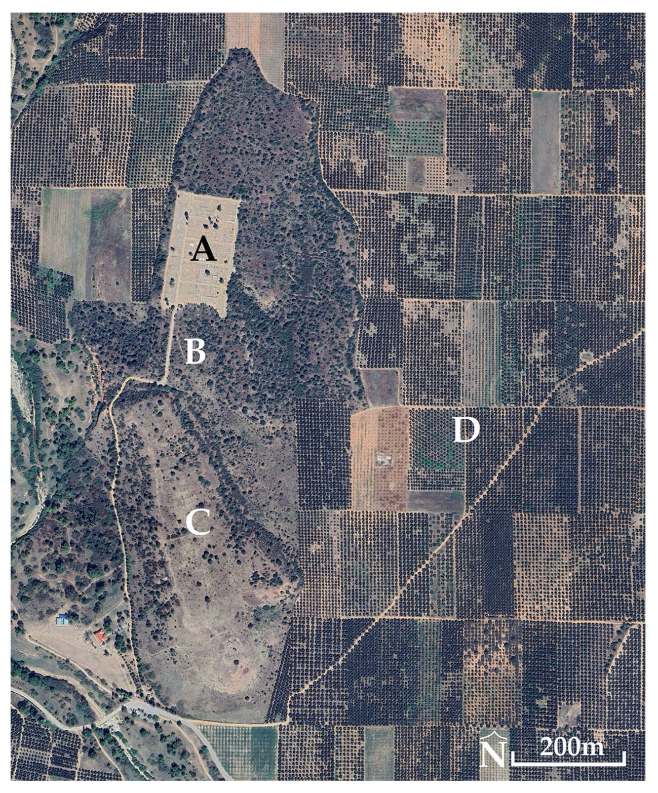
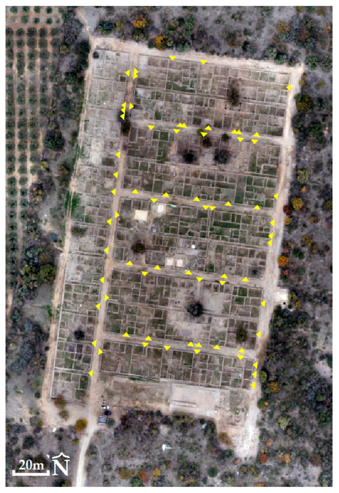
A total of 20 GCPs and 20 CPs were surveyed (Figure 3). The collection process of the X, Y, and Z coordinates within the Greek Geodetic Reference System 1987 (GGRS87) involved the use of 24 × 24 cm paper targets (Figure 3) and the Topcon HiPer SR GNSS receiver (Topcon Positioning Systems, Tokyo, Japan), which provided real-time kinematic (RTK) positioning and a network of permanent stations provided by Topcon, with an accuracy of 1.5 cm horizontally and 2 cm vertical.

In relation to the GNSS measurements (using the Topcon HiPer SR GNSS receiver, Topcon Positioning Systems, Tokyo, Japan) associated with the UAS’s PPK system, the x, y, and z coordinates of a randomly selected point, designated as the reference for subsequent measurements, were initially determined with 1.5 cm horizontal and 2.0 cm vertical accuracy in the GGRS87 system. This measurement was conducted near the UAS home position using the RTK method. Following this, the same GNSS device was employed at the same location to continuously record position data using the static method 30 min before the flight, throughout the flight, and for an additional 30 min post-flight. By integrating the high-precision coordinates of this reference point, its static measurements, and in-flight data from the UAS’s built-in multi-frequency PPK GNSS antenna, the reception center coordinates (X, Y, and Z) for each captured image were adjusted and computed during post-processing. This was carried out using the WintraHub© v2.17.0 software from the UAS manufacturer, ultimately achieving a 3D positional accuracy within GGRS87 of 2 cm horizontally and 3 cm vertically for each image.

5.3. Production of DSMs and Orthophotomosaics

The UAS images were processed in the software Agisoft Metashape Professional© version 2.0.3. In the software, initially images are imported, and the GGRS87 coordinate system is established. In cases where the MS images are used, it is essential to calibrate the spectral data right after importing the images. To do this, calibration targets are imaged both before and after the flight. The software then automatically detects these targets and calculates the reflectance values for all spectral bands [15,16,17,18,19].

Next, whether you are using an RGB or MS sensor, the images are aligned with high precision. This alignment process also generates a sparse point cloud by matching groups of pixels across the images. If Ground Control Points (GCPs) are incorporated, the next step involves identifying and marking them on each image. Once that is complete, the software calculates the Root Mean Square Error (RMSE) for the x coordinate (RMSE_x) as well as for y and z coordinates (RMSE_y and RMSE_z), along with combined RMSE values for the x and y coordinates (RMSE_xy) and for all coordinates (RMSE_xyz), and for all GCP Locations [20].

If GCPs are not used, the process relies on the pre-calculated coordinates of the image centers. After aligning the images and generating a sparse point cloud, the software computes RMSE values for the sensor locations, that is RMSE_X for the X, RMSE_Y for Y, RMSE_Z for Z coordinate, and the combined values RMSE_XY and RMSE_XYZ.

These RMSE figures provide a rough indication of the overall accuracy of the resulting DSMs and orthophotomosaics (though they rarely match the true accuracy of the final products).

Following this, with either sensor type, the next step is to build a dense point cloud using high-quality settings and aggressive depth filtering (121,415,757 points for the RGB and 6,668,369 points for the MS). This dense point cloud is then converted into a 3D mesh (triangular mesh). After the mesh is generated (source data: point cloud; surface type: Arbitrary 3D; face count for the RGB: high 32,000,000; face count for the MS: high 1,800,000; and production of 81,006,681 faces for the RGB and 4,022,716 faces for the MS), a texture is applied (RGB or MS texture type: diffuse map; source data: images; mapping mode: generic; blending mode: mosaic; and texture size: 16,284), effectively overlaying the colored details onto the 3D surface. The final step involves producing a DSM and an orthophotomosaic.

In the case of the ancient Olynthus using RGB images, the RMSE_xyz was 1.6 cm when GCPs were employed, while the RMSE_XYZ was 3.2 cm when GCPs were not employed. Regardless, the resulting products achieved a spatial resolution of 2.6 cm for the DSM (

Table 1. Results in Agisoft Metashape Professional© and the spatial resolutions (all in cm) of the products.

Sensor	Use of	RMSE										DSM	Ortho
		x	X	y	Y	xy	XY	z	Z	xyz	XYZ
RGB	GCPs	1.1		0.9		1.4		0.9		1.6		2.6	1.3
RGB	PPK		1.1		2.9		3.1		0.9		3.2
MS	GCPs	0.8		0.6		1.0		0.3		1.0		12.2	6.1
MS	PPK		0.3		0.4		0.5		0.9		1.0

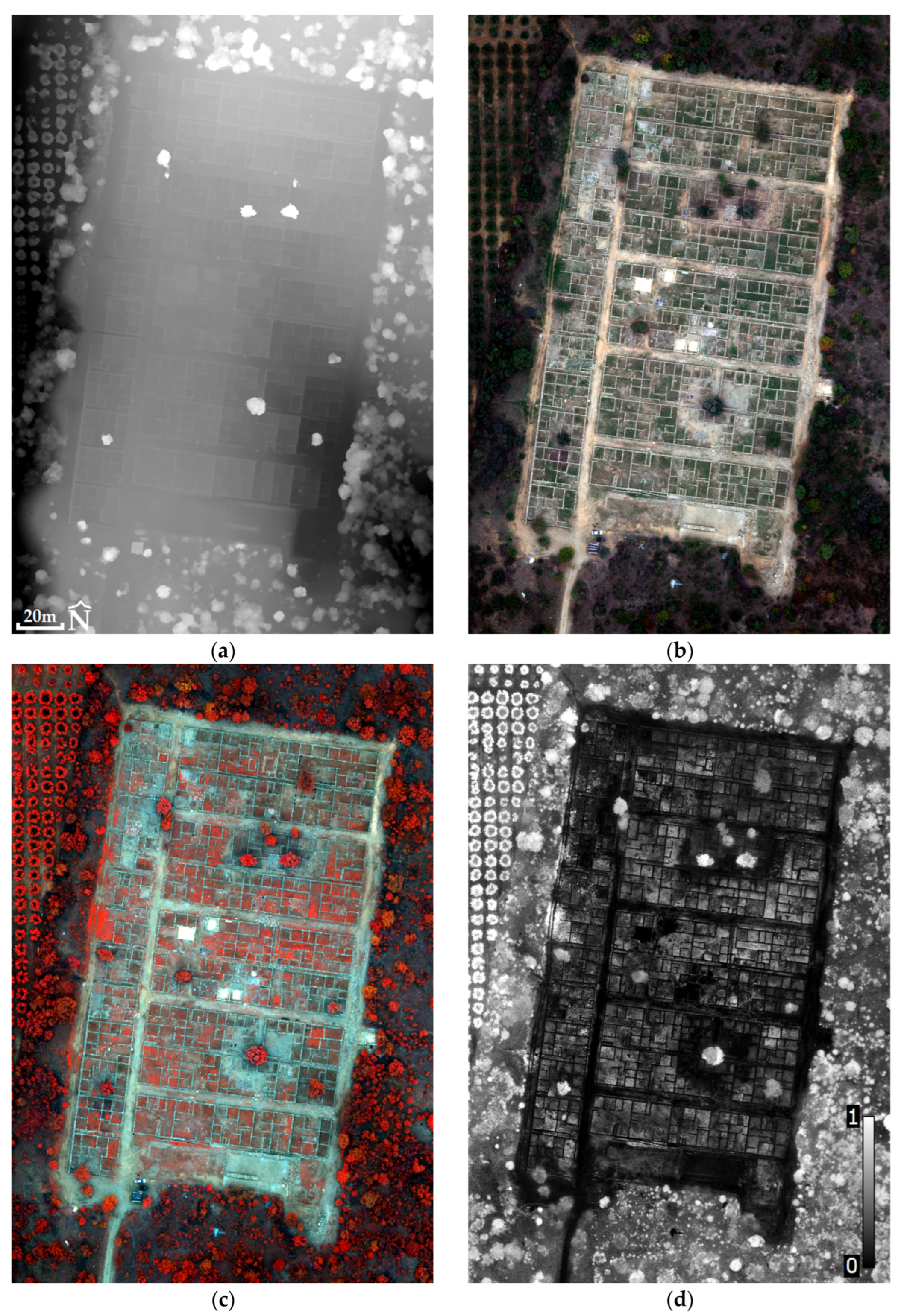
) and 1.3 cm for the orthophotomosaic in both scenarios. For the MS images, the RMSE_{xyz or XYZ} was 1 cm when GCPs were or were not employed. The final products have a spatial resolution of 12.2 cm for the DSM (Figure 4) and 6.1 cm for the orthophotomosaic in both scenarios.

In Figure 4, the Normalized Difference Vegetation Index (NDVI) is presented [15,21]. The grayscale of the images ranges from zero (black) to one (white), with zero representing the least favorable and one representing the most favorable outcome of the index. That is, a value of 0 corresponds to pixels without crop, a value of 0.5 corresponds to pixels with poor growth or poor crop health, and a value of 1 corresponds to pixels with good growth or healthy crop.

5.4. Control of DSMs and Orthophotomosaics

The RGB images were processed twice, once with the use of GCPs and once without the use of GCPs. The same was performed for the MS images. For each of the four processing cases, the final products produced were DSM and an orthophotomosaic. By extracting the coordinates (x’, y’, and z’) of the CPs from the products for the four processing cases, it was possible to compare them with the coordinates (x, y, and z) of the CPs in the field to evaluate the quality of the products.

The mean value is determined by summing the differences between the coordinates of the CPs obtained from the products and those recorded in the field and then dividing this total by the number of CPs. However, because relying solely on the mean is not enough to draw conclusions, the standard deviations were also calculated. This measure quantifies how much Δx, Δy, and Δz vary from their respective mean values. Naturally, we expect these standard deviations to be as low as possible and definitely smaller than the corresponding mean values.

In addition to using a standard histogram to visualize the data distribution, we performed several diagnostic tests, including assessments of Variance Equality, Skewness, and Kurtosis. All of these tests confirmed that our data were normally distributed, which allows the utilization of analysis of variance (ANOVA).

ANOVA is used to conduct hypothesis tests that compare the mean values across different datasets. Specifically, the null hypothesis (H₀) assumes that the samples, whether they come from product measurements (x, y, and z) or field measurements (x’, y’, and z’), have the same mean. In contrast, the alternative hypothesis (H_A) suggests that at least one of the means is different. If the p-value exceeds 0.05 at a 95% confidence level, it indicates that there is no systematic difference between the product-derived means (x, y, or z) and the corresponding field measurements (x’, y’, or z’). In such cases, any observed differences are considered negligible and attributed to random errors. Also, if the calculated F statistic is lower than the critical value (F crit), it implies that the standard deviations for the product and field measurements do not differ significantly, reinforcing the conclusion that the variations are simply due to random error [6].

The tables below present the mean values and standard deviations (

Table 2. Mean values and standard deviations (all in cm) of CPs for the two processing cases.

Sensors	Processing Cases	CPs (x′, y′, z′ Values in Products; x, y, z Field Measurements)
		Δx = |x′ − x|		Δy = |y′ − y|		Δz = |z′ − z|
		Average Value	Standard Deviation	Average Value	Standard Deviation	Average Value	Standard Deviation
RGB	GCPs	1.0	0.9	0.7	0.6	1.7	1.5
	PPK	1.8	0.9	0.7	0.6	10.6	2.4
MS	GCPs	1.1	0.9	1.0	0.9	2.6	1.7
	PPK	1.3	1.2	1.2	1.1	7.0	2.7

) along with the ANOVA results (

Table 3. ANOVA. Comparison of x and x′, y and y′, and z and z′ of CPs (using GCPs).

Sensors	Source of Variation (Between, Within Groups = BG, WG)		Sum of Squares	Degrees of Freedom	Mean Square	F	p-Value	F Crit
RGB	x and x′	BG	0.00021	1	0.00021	1.1 × 10−7	0.99974	4.09817
		WG	71,529.74626	38	1882.36174
		Total	71,529.74647	39
	y and y′	BG	5.0625 × 10−5	1	5.0625 × 10−5	1.01 × 10−8	0.99992	4.09817
		WG	191,000.9797	38	5026.34157
		Total	191,000.9797	39
	z and z′	BG	0.00058	1	0.00058	12 × 10−5	0.99148	4.09817
		WG	189.80601	38	4.99490
		Total	189.80659	39
MS	x and x′	BG	0.00022	1	0.00022	1.2 × 10−7	0.99973	4.09817
		WG	71,545.36495	38	1882.77276
		Total	71,545.36517	39
	y and y′	BG	4 × 10−5	1	4 × 105	8 × 10−9	0.99993	4.09817
		WG	191,001.5658	38	5026.35699
		Total	191,001.5658	39
	z and z′	BG	9 × 10−9	1	9 × 10−6	1.8 × 10−6	0.99894	4.09817
		WG	190.74630	38	5.01964
		Total	190.74631	39

and

Table 4. ANOVA. Comparison of x and x’, y and y’, and z and z’ of CPs (using PPK).

Sensors	Source of Variation (Between, Within Groups = BG, WG)		Sum of Squares	Degrees of Freedom	Mean Square	F	p-Value	F Crit
RGB	x and x′	BG	0.0024	1	0.00243	1.3 × 10−6	0.9991	4.09817
		WG	71,535.57947	38	1882.51525
		Total	71,535.5819	39
	y and y′	BG	3.24 × 10−5	1	3.24 × 10−5	6.4 × 10−9	0.99994	4.09817
		WG	191,009.1297	38	5026.55605
		Total	191,009.1298	39
	z and z′	BG	0.11230	1	0.11300	2.26 × 10−2	0.88131	4.09817
		WG	190.03895	38	5.00103
		Total	190.15195	39
MS	x and x′	BG	0.00010	1	0.00010	5.4 × 10−8	0.99982	4.09817
		WG	71,532.1653	38	1882.42540
		Total	71,532.1654	39
	y and y′	BG	8 × 10−5	1	8 × 10−5	1.6 × 10−8	0.99990	4.09817
		WG	190,987.5981	38	5025.98942
		Total	190,987.5981	39
	z and z′	BG	0.049	1	0.049	98 × 10−4	0.92166	4.09817
		WG	190.00717	38	5.00019
		Total	190.05617	39

).

5.5. Production and Control of the Fused Image

The UAS is not equipped with a Panchromatic (PAN) sensor that is integrated into satellite platforms to capture high-resolution grayscale images. At first glance (Table 2), the best spatial accuracy is achieved when using GCPs (analysis will be completed in the Discussion). Following the satellite image processing workflow for image fusion [22,23,24,25,26,27,28], the available high-resolution RGB orthophotomosaics (from UAS, use GCPs) are transformed into pseudo-panchromatic (PPAN) orthophotomosaics (Figure 5). The process involves utilizing image processing software Adobe Photoshop© CS6 version 13.0 to transform the full-color RGB image into a black and white (B/W) image. The intensity (or brightness) of each pixel is calculated by preserving predetermined ratios among the three primary color channels (red, green, and blue). The precise algorithm employed by software to achieve this conversion remains undisclosed due to copyright restrictions. Consequently, while the PPAN image bears a visual resemblance to those produced by an authentic PAN sensor, they do not exhibit the identical spectral characteristics that PAN sensor, which are sensitive to the entire visible spectrum, are designed to capture.

Following the conversion to a PPAN image, further processing steps are implemented to refine the fusion process. Specifically, the histogram of the PPAN orthophotomosaic is adjusted so that they align with the corresponding MS orthophotomosaic. This histogram matching process plays a critical role in ensuring that the tonal distribution in the PPAN image mirrors that of the MS image, thereby reducing discrepancies and facilitating a more seamless integration of the spectral data.

Numerous methods have been proposed for fusing MS and PAN images. These techniques generally fall into three categories: component substitution (CS), multiresolution analysis (MRA), and degradation model (DM)-based methods. CS approaches use transforms, such [28,29,30] as intensity-hue–saturation (IHS), principal component analysis (PCA), and Gram–Schmidt, to project interpolated MS images into a new domain. In this space, one or more components are partially or completely replaced by a histogram-matched PAN image before applying an inverse transform to reconstruct a MS image (in other words, a fused image). MRA techniques [24,28,30,31,32,33] operate on the assumption that the spatial details missing in MS images can be recovered from the high-frequency components of the PAN image, a concept inspired by ARSIS (Amélioration de la Résolution Spatiale par Injection de Structures) [34]. Tools such as the discrete wavelet transform, support value transform, and contourlet transform are employed to extract spatial details, which are then injected into the MS images. Some methods also incorporate spatial orientation feature matching to improve correspondence. DM methods [24,25,26,27,28] model the relationships among MS, PAN, and fused images by assuming that MS and PAN images are generated by down sampling and filtering an underlying fused image in the spatial and spectral domains, respectively. These approaches integrate priors such as similarity, sparsity, and non-negativity constraints to regularize the fusion process.

In this research, with use of the software Erdas Imagine© version 16.7.0, the principal component analysis (PCA) method was used to generate the fused image (Figure 6). PCA is a robust statistical technique that extracts and combines the most significant components from the datasets, merging the detailed spatial information provided by the PPAN image with the rich spectral information inherent in the MS image. To evaluate the success of the fusion process, the correlation table was constructed to compare the MS orthophotomosaic with the fused image (

Table 5. Correlation table.

		MS Orthophotomosaic					Fused Image (FI)
		Bands
		1	2	3	4	5	1	2	3	4	5
MS	1	1	0.978	0.959	0.890	0.447	0.786	0.782	0.738	0.748	0.286
	2	0.978	1	0.972	0.941	0.530	0.735	0.770	0.721	0.774	0.363
	3	0.959	0.972	1	0.914	0.426	0.753	0.782	0.784	0.782	0.264
	4	0.890	0.941	0.914	1	0.691	0.573	0.636	0.591	0.766	0.51
	5	0.447	0.530	0.426	0.691	1	0.098	0.185	0.077	0.411	0.904
FI	1	0.786	0.735	0.753	0.573	0.098	1	0.979	0.956	0.861	0.176
	2	0.782	0.770	0.782	0.636	0.185	0.979	1	0.972	0.922	0.27
	3	0.738	0.721	0.784	0.591	0.077	0.956	0.972	1	0.895	0.157
	4	0.748	0.774	0.782	0.766	0.411	0.861	0.922	0.895	1	0.493
	5	0.286	0.363	0.264	0.510	0.904	0.176	0.270	0.157	0.493	1

). These tables indicate the retention rate of the original spectral information, which should exceed 90% (i.e., correlation values greater than 0.9) [35,36,37].

The ERGAS (Erreur Relative Globale Adimensionnelle de Synthese) index (Equation (1)) is a well-established metric for quantitatively assessing the quality of a fused image in relation to the (original) MS orthophotomosaic [38].

In Equation (1), the variable “h” represents the spatial resolution of the fused images,

$$\mathrm{E}\mathrm{R}\mathrm{G}\mathrm{A}\mathrm{S}=100{\displaystyle \frac{\mathrm{h}}{\mathrm{l}}}\sqrt{{\displaystyle \frac{1}{\mathrm{N}}}\sum _{\mathrm{k}=1}^{\mathrm{N}}\left[{\displaystyle \frac{\mathrm{R}\mathrm{M}\mathrm{S}\mathrm{E}({\mathrm{B}}_{\mathrm{k}}{)}^2}{({\mathrm{M}}_{\mathrm{k}}{)}^2}}\right]}$$

(1)

while “I” denotes the spatial resolution of the MS images. “N” indicates the total number of spectral bands under consideration, and “k” serves as the index for each band. For every band in the RMSE(B_k) (Equation (2)) between the fused image and the MS image, “M_k” represents the mean value of the “k” spectral band.

$$\mathrm{R}\mathrm{M}\mathrm{S}\mathrm{E}\left(\mathrm{B}\right)=\sqrt{{\displaystyle \frac{{\sum }_{\mathrm{i}=1}^{\mathrm{n}}{({\mathrm{P}}_{\mathrm{i}}-{\mathrm{O}}_{\mathrm{i}})}^2}{\mathrm{n}}}}$$

(2)

In Equation (2), for each spectral band, the values labeled “P_i” for the MS image and “O_i” for the fused image, are obtained by randomly selecting a number (“n”) of pixels at the same coordinates from both images. This pixel-by-pixel comparison is essential to ensure an unbiased overall assessment of spectral fidelity.

The acceptable limits for ERGAS index values, which determine the quality of the fused image, are not fixed and can vary depending on the specific requirements of the application. For instance, when high spectral resolution is crucial, very low index values may be necessary. In other scenarios, moderate index values might be acceptable, especially if external factors (such as heavy cloud cover or high atmospheric humidity) affect the quality of the fused image. Additionally, these limits depend on the number and spatial distribution of the pixels tested, as well as on the researcher’s criteria for acceptable error on a case-by-case basis. Lower ERGAS index values, especially those close to zero, indicate a minimal relative error between the fused image and the MS orthophotomosaic, suggesting a high-quality fusion. Moderate values, typically between 0.1 and 1, imply that although there might be slight spectral differences, the fused image remains acceptable. High index values, generally ranging from one to three, denote significant relative error and considerable spectral deviation, classifying the fused image as low quality. Despite these general guidelines, the thresholds can be adjusted; however, the index is usually maintained below three for a fused image to be reliably used for further classification or detailed analysis [38,39,40,41,42,43,44,45,46,47,48].

At the ancient Olynthus, 68 million pixels out of a total of 290 million from the fused image were analyzed using the Model Maker tool in Erdas Imagine© version 16.7.0 to compute the ERGAS index. The resulting value was 0.8, and this moderate error suggests that, while minor spectral differences exist, the overall quality of the fused image is good.

6. The Hippodamian System of Ancient Olynthus

Using orthophotomosaics and with review of the literature, the following paragraphs offer a concise overview of the Hippodamian system of the excavated part of ancient Olynthus.

6.1. The City Blocks

The ancient city of Olynthus extended from the southern hill (position C, Figure 7) which was the initial site of the settlement, to the northern hill (position A, Figure 7), where the settlement expanded, and to the area of the villas (position D, Figure 7) which later became the eastern suburb of the settlement [49].

The governance of ancient Olynthus was based on the principles of freedom, isopolitics, democracy, and mutual respect [50]. This is evident in the design of the North Hill extension, which was based on the principles of the Hippodamian system. The city (position A, Figure 7) is split into city blocks using a system of parallel and vertical road axes, which are equal in size, with isometric residences, while the spot reserved for public buildings is entirely separate. The residences of the North Hill were built gradually, starting from the south towards the north. The city blocks between the avenues A and B (Figure 8) measured 86 × 36 m. Every city block consists of ten houses, organized in two rows, five north and five south, with a public cobbled sewer pathway between [51]. A differentiation in design can be observed along the western border of the city and Avenue A, where a line of residences can be seen, in contrast with the south city block, which consists of only one line of residences. Each residence has a floor plan area of about 300 m² [49].

6.2. Road Arteries

The arteries which were directed north to south were named “Avenues” (Avenues A and B, Figure 8). The arteries which were directed west to east where named “Streets” and have roman numerals V to VIII. The name of each city block is derived from a combination of the avenue and road name at the southwest corner of the city block. Within the city blocks, the buildings are numbered from left to right. The buildings located in the north line were named utilizing odd numbers, while the buildings of the south line using even numbers. Avenue A has a width of about 5 m, while Avenue B has a width of about 7 m. The roads had parts made of cobblestone, in order to smooth natural slopes, to deal with static problems of the adjacent buildings and ensure the comfortable passage of carriages. There also existed raised side belts, with a goal to aid in the passage of pedestrians [49,50,51,52].

6.3. Typology of Buildings

The part of Olynthus, which is being discussed, consists of private residences. Inside these residences, apart from the main rooms of the house, there were also spaces that operated as workshops and shops. The workshops served the purpose of providing a space to construct objects for in-house use or objects that were meant to be sold. The economic activities of the household also affected its size. A typical Olynthian building was divided by two main axes, parallel in the east–west direction. One of the axes was near the middle of the building, resulting in its division into two almost equal parts, while the second annex was located in the northern half of the building, resulting in its subdivision into two smaller parts (Figure 9) [50].

The buildings had entrances which faced the side of the street, with an entrance for pedestrians and, sometimes, a second bigger entrance meant for carriages. The entrances of the houses located in the northern line were usually located in the north side of the buildings, facing the street. The buildings located in the south line had entrances in the south side facing the corresponding street, with an exception for the houses present in the corner of the city blocks, which faced the vertical streets (Figure 10). The residences that included shops had extra entrances on the side of the road, making the entrance of customers easy [51].

While the houses are not preserved to any height, bibliography proves that the houses had one or two floors and were mixed within the city blocks without a specific division. The evidence of the existence of a second story in the house becomes perceptible mainly by the stone staircase that survive in many houses and, less directly, by the pillared partitions in kitchen complexes, which must have supported a wall above the room. All houses in a row or a block tended to have the same number of stories in order to carry a common roof line, but this was not the norm. For example, four of the five houses in the southern row of block Avii retain staircases. This row appears to have had a second story, whereas the row to the north did not. In block Av, however, only houses Av6, Av9, and Av10 have staircases. Most of the houses with a second story use the rooms of that floor as guest rooms, the couple’s bedroom, and rooms for the slaves. The wealthier families usually owned bigger and more complex houses, featuring multiple rooms. In contrast, the families bellowing in the lower economic class owned smaller, simpler homes, which covered their basic living needs [50]. According to Hoepfner [53], there exist some variations in the typology that occur less frequently and differ in the interior design of the residences (Figure 11).

6.4. Morphology of Buildings

Olynthian homes share a lot of common design points; however, each of the buildings is unique and different. The typical Olynthian household was usually of square plan with a side of about 17 m and belonged to the type including “pastas”, which refers to a covered arcade in the inside of the home, which was supported by wooden columns and used for the everyday household chores [49]. On the ground floor, eight to thirteen rooms were present, which were organized around an outdoor cobblestone courtyard (Figure 9). The courtyard was the most prevalent light source of the home, it had a well or small tanks which stored water, and in the middle the omen of Zeus Erkios was present. Pastas was in the northern end of the courtyard. The pastas was connected to the north with three or four rooms, the “diatitiria”, which were used to host strangers. The central entrance of the home led to the courtyard through a lobby. Many of the homes had a second floor, which was connected to the courtyard through a wooden staircase. This design allowed for the light to diffuse, the temperature of the home to be conserved, and for the best possible flow inside the home [51,52].

In detail, to divide the indoor parts of the home and their use, every house, regardless of its size, was composed of some common types of rooms, which were crucial to ensure the proper functioning of the family. Firstly, there existed a big room named “oikos” and two smaller ones in the immediate vicinity, the “kapnodoki” (smokestack) and the “valanio” (bath) (Figure 9). The house measured about 4.5 m × 5.5 m, and inside there existed a stone hearth for heating in the winter. The bath included a curated sewerage system with clay baths and basins [52]. The “kapnodoki” was a small rectangular room with a roof designed as a chimney, which reached above the roof and was used to divert the smoke to the outside and to air the home. These three rooms were divided between them using a series of columns [49].

Next in line is the “Andron” (Figure 9) which was used for the symposiums of men. It was a square space with dimensions close to about 4.8 × 4.8 m². It was the most formal room in the home, decorated with painted walls and mosaic floors. The entrance to the “Andron” was possible through an antechamber, and it was usually located next to an interior wall in the corner of the home, so it could be illuminated through the larger windows in the house [51].

Between the rest of the areas of the home, the “pitheons” stood out. They were places used to store olive oil, wine, wheat, and other raw materials, workshops with wine presses, sanders, and looms, as well as spaces meant to keep animals [52].

The courtyard was the center of the home. It was usually the biggest space in the house, which aided in connecting the rooms and promoting a sunny interior. The courtyard provided light into the closed spaces of the home through windows. The size of the room differed from a small 10–15 m² space to 100 m². This means that the courtyard took up to 3% to 34% of the total square area of the home. The floor was either cobblestone, rock, or mosaic. Often, they were equipped with sewage systems to drive dirty water into the road. Some houses had vases meant to collect rainwater from the gutters, which was then used to wash clothes and other household chores [50].

Some houses had rooms with a door on the side of the road, and their use was attributed to the existence of shops or workshops. Many shops had openings towards the inside of the home. The incorporation of the workshops into the homes was efficient and supported the local economy, keeping businesses within residential neighborhoods [51].

6.5. Particular Typological and Morphological Features

The home (οίκος) and the pastas (στοά), appeared to be the places that took up the majority of a typical Olynthian household, considering these elements were supporting the whole household, since a lot of work took place in these spaces. On the other hand, the houses A11, A10, A9, A8, A7, Aiv9, Av9, Av10, Avi9, Avii10, Avii9, Aviii9, and Aviii10 (Figure 8 and Figure 12) had stores in their interior or workshops that covered an average of a quarter of the house’s total square footage. Almost all the homes mentioned were located along Avenue B, with their shop’s entrance facing the street, creating a separate group (shop zone). The rest of the houses that featured stores (the ones in line A) are located along Avenue A (Figure 8 and Figure 12). The placement of these shops with their entrance towards the avenue was not random, since Avenue B was operating as a central shopping artery of markets and trade. In addition, on Avenue A, more workshops can be observed [50].

The home Av6 (Figure 8) is an interesting example to study, since it is bigger in size than the rest. It had a square footage of about 430 m², and it took the area of the next-door property (Av8) [49].

According to relevant bibliography, the houses of city block Avi (Figure 8) are the most luxurious, when compared to the rest. Most of the homes featured colored walls, the flooring, particularly inside the Androns, were mosaic, and some of these homes featured a second floor. In the series of homes A2 to A13 (Figure 8), their dimensions are about 16.5 × 21.0 m², and their orientation is east–west. Houses A6 and A7 (Figure 8) were an exception to the rule, since the first does not follow the classic dimensions, and it takes up part of the property belonging to home A7, leaving it a smaller area. Their entrances faced Avenue A and had a cobblestone path in their south part, which was meant to drive stormwater away from the courtyards [49].

6.6. The Economy

The majority of the residents of Olynthus were engaged in agriculture. However, trade and craftsmanship were also a big part of the economy, as shown by the existence of workshops inside the homes and the shops and the equipment present inside the workshops [50].

Among the economic strategies followed by the inhabitants of the city, the one that stood out the most was household economy and self-sufficiency, according to which, the families produced a big part of their food, fabrics, and ceramics. There existed also the strategy of specialization and production for sale, according to which, some houses focused on specific craft activities [50]. Usually, houses with shops in Avenue B had also workshops. These workshops either channeled their products to their own shops cause this avenue was the most commercial street or kept them for private use.

The wealthiest families appeared to be focused on storing and managing resources, while the weakest ones held workshops in their houses, a fact that proves that they relied on immediate production for their survival [50].

The homes that included workshops created vessels for everyday use and for trading, tools, weapons, and decorative objects made of copper and iron. There were olive oil mills and wineries that were used for agricultural production, showing the importance of agriculture and the processing of agricultural products. Some textile workshops existed too, producing fabrics for domestic and commercial use [51].

What is most fascinating regarding Olynthus is not the existence of different economic activities, but their complementary, almost mutually exclusive distribution in space. For example, the houses Aiv9 andAv9 (Figure 8) produced lots of fabrics, while the houses A6, Av10, Avi10, and Avii9 (Figure 8) processed agricultural items [50].

Houses around the agora were sold more often, and they were significantly more expensive than the others. The most expensive were the house Av10 and Aiv3 (Figure 8) [51].

For example, the houses Aiv9 and Av9 (Figure 8) produced a large number of fabrics while houses A6, Av10, Avi10, and Avii9 contained spaces meant to process agricultural products. In houses Avi8 and Avi10, processing facilities of agricultural materials and grape processing were found [50].

7. Discussion

According to the above results of both RGB and MS sensor image processing (Table 3 and Table 4), with and without the use of GCPs, the p-values consistently exceeded 0.05. This indicates that, at a 95% confidence level, there appears to be no systematic error between the mean x (or y or z) values of the CPs of the products and the (actual) mean x (or y or z) values of the CPs measured in the field. Thus, any differences between them are considered negligible and are attributed to random errors.

In addition, the F test was found to be lower than its critical value (F crit) in all cases. The standard deviations of x′ (or y′ or z′) and x (or y or z) do not differ significantly, so that the measurements (field and product) are accompanied only by random errors. All the above justifies a deeper analysis of the mean differences and standard deviations between the 3D coordinates of the two data sources.

Table 2 reveals that, in both processing scenarios for both sensors, the standard deviations of the differences in CP measurements are consistently lower than the corresponding mean differences (on the three axes). This finding demonstrates that the dispersion of Δx, Δy, and Δz around their mean values is limited.

Focusing on horizontal accuracy, the average difference between the CP measurements is approximately 1 cm in both cases (whether GCPs are employed or not, for both sensors). This result aligns with the manufacturer’s specification, which anticipates a horizontal accuracy of around 1 cm for RGB sensor imagery processed without GCPs [13].

Turning to vertical accuracy, the results are varied. When GCPs are used, the average vertical differences are 1.7 cm for the RGB sensor and 2.6 cm for the MS sensor, results that are even better than theoretically expected (theoretically about three times worse than the horizontal accuracy).

On the contrary, processing that relies solely on PPK produces less favorable results. In the case of the MS sensor, the average value of the CP differences is 7 cm, which is two times worse than the theoretically expected. In the case of the RGB sensor, the average value of the CP differences is 10.6 cm, which is over three times worse than the theoretically expected.

Generally, when using PPK for the georeferencing of UAS imagery, the image-center positions exhibit very high relative planimetric accuracy, but the images remain sensitive to small vertical errors. This sensitivity arises primarily because the acquisitions are nadir and the intersecting optical rays form very shallow angles with the vertical plane. As a result, there is little perspective on ground objects, so small errors in elevations of the image-centers translate into larger elevation errors on terrain features. Furthermore, in PPK solutions, factors such as the number of tracked satellites, the satellite geometry (i.e., how well the satellites are distributed across the sky) and atmospheric delays (ionospheric signal dispersion and tropospheric water vapor and pressure) disproportionately affect the vertical component. However, when GCPs are employed, these issues are overcome, since GCPs provide fixed ground points at known accurate elevations. Thus, even if the optical rays intersect at shallow angles, the GCPs anchor the DSM to the true ground level, substantially limiting the elevation errors of surface features.

The question of interest when improving the spatial resolution is whether the spectral information of the MS orthophotomosaic is preserved in the fused image. According to the correlation table (Table 5), the spectral information of the MS orthophotomosaic is transferred to the fused image at an average percentage of 78% for blue—green—red—Red Edge bands. The percentage of the spectral information of the NIR band transferred is 90%. In general, when a percentage below 90% is observed in any correlation of corresponding bands, then the fused image is not acceptable for classification. On the other hand, the above percentages are objectively not low, and therefore the ERGAS index should be used so that, in combination, reliable conclusions can be drawn.

In summary, there were challenges that had to be addressed to ensure the quality of the fused image, and the main ones are presented below. First, the RGB and MS images had to have spatial alignment (the images should perfectly match spatially when one covers the other) in GGRS87, otherwise the spectral information transferred from the MS to the fused image would have been greatly corrupted. This was successfully overcome, since the processing of the images (RGB and MS), whether using GCPs or not, led to orthophotomosaics with high planimetric accuracy (approximately 1 cm). Also, another important challenge was the radiometric deviation of the produced PPAN orthophotomosaic from the MS orthophotomosaic. This was addressed by performing histogram matching of the PAN image to the MS orthophotomosaic. Finally, a further challenge was preserving the spectral information of the original MS orthophotomosaic in the fused image. This was managed by creating and evaluating the correlation table and by calculating and assessing the ERGAS index.

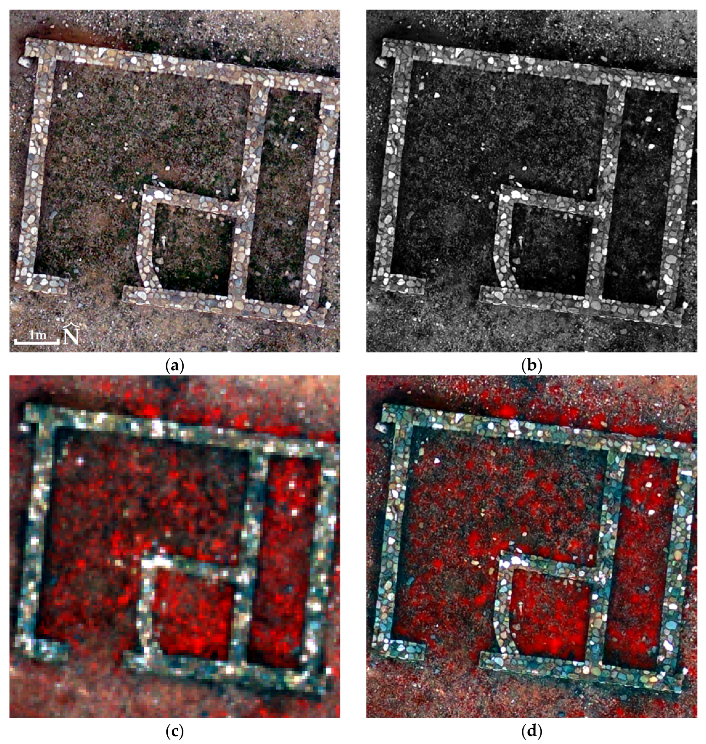
If the RGB and fused images are compared (see Figure 6a,d,e,h), it becomes apparent that, although the spatial resolutions of the images are identical, the spectral information is superior in the fused images, thereby enabling automatic detection of different objects when classification techniques are applied. For example, in Figure 6a it is difficult to detect and distinguish vegetation, whereas in Figure 6d the areas occupied by vegetation are clearly delineated (pixels shown in red). Furthermore, if the MS and fused images are compared (see Figure 6c,d,g,h), it emerges that, while their spectral information is similar, the spatial resolution is superior in the fused images, thus permitting both improved and more comprehensive visual observation of objects and greater accuracy in identifying different objects when applying classification techniques. For example, in Figure 6.g it is difficult to discern the mosaic motifs, such as the rays of the Vergina Sun, whereas in Figure 6d all mosaic motifs are clearly visible.

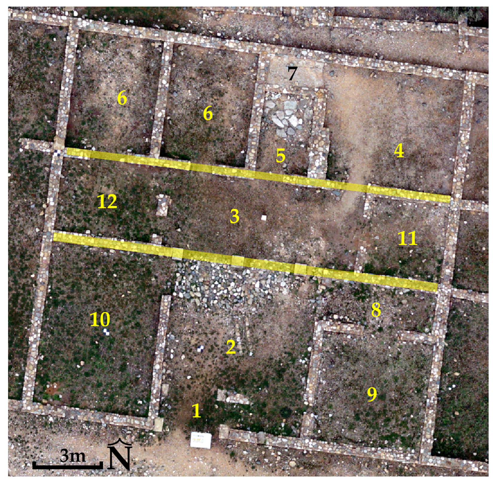
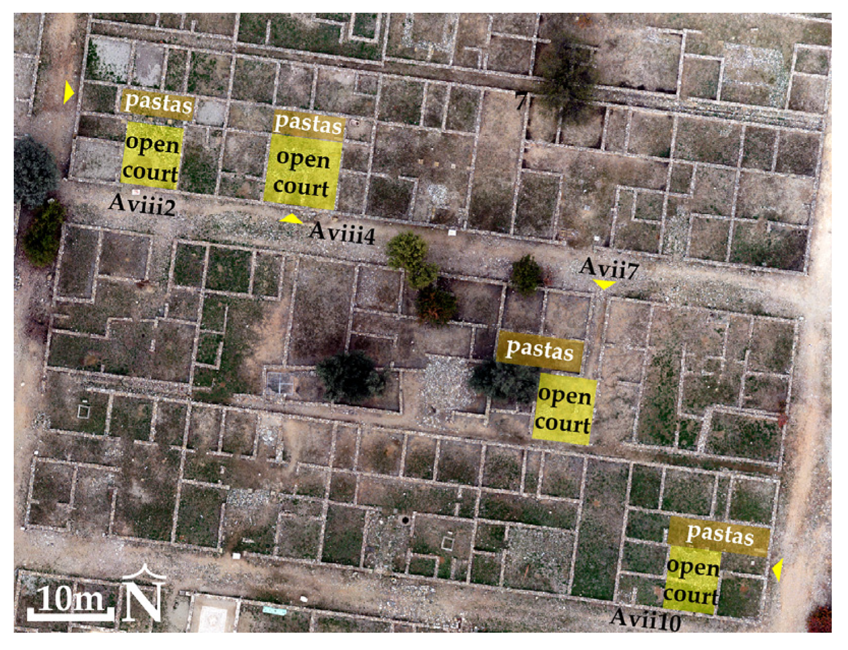
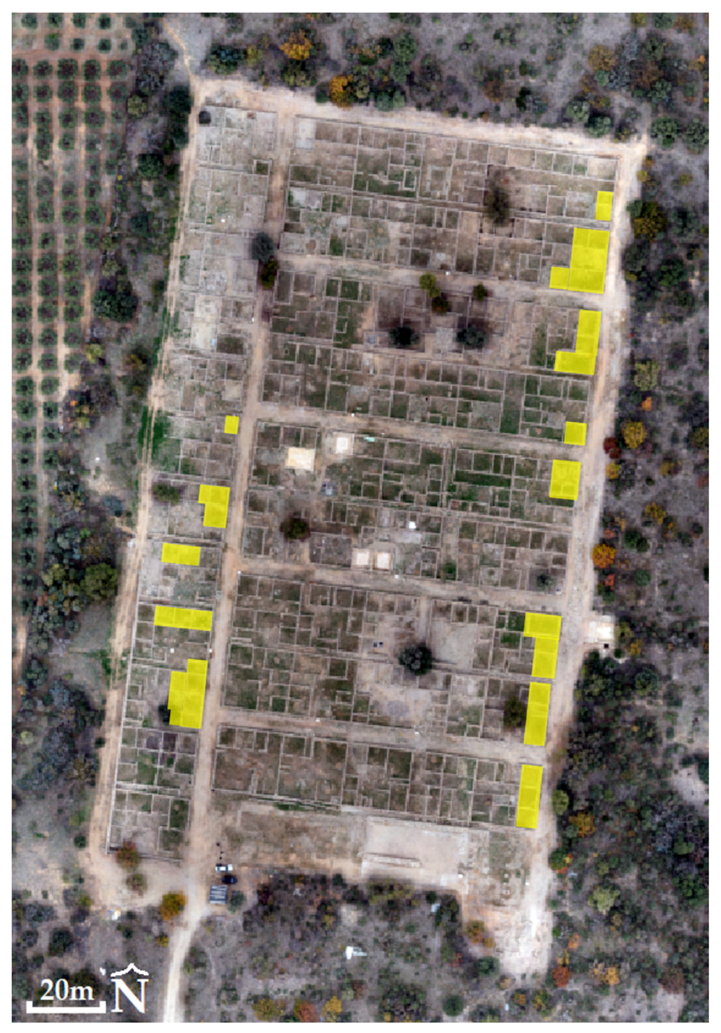
From the study of the Hippodamian system of ancient Olynthus, it follows that the carefully designed urban grid was not merely an aesthetic endeavor but also played a crucial role in the community’s functioning. The organized layout of the city provides valuable insights into its urban structure as well as the prevailing socio-economic relationships. However, despite the advantages the Hippodamian system provides, there are some limitations that govern it. First, there is the adaptation of the design to the natural landscape, such as the slopes of the settlement. Bibliography reports that there were equal building blocks on the flat part of the hill and slightly smaller ones on the eastern slopes, following the morphography of the terrain [49]. Also, another limitation is the size of the buildings. In particular, the Hippodamian system, despite the organization it offers to the settlement, also promotes the principles of egalitarianism. This means that the inhabitants of ancient Olynthus, regardless of their economic status, were all required to have the same building area. Finally, there were defense disadvantages as the horizontal and vertical streets of the city made it easily accessible to enemies in case of invasion, unlike a more labyrinthine city, whose defense would have been more reinforced. Data reveal a well-structured network of road axes and building blocks, and the examination of building dimensions and internal configurations shows how architectural design mirrored the social structures of the era. Additionally, the placement of workshops and shops confirms the interaction between private production and collective economic activities in the city. The presence of a shop in a house did not reflect the economic status of a household. The wealthier households were mixed within the blocks, and their economic status was revealed by the existence of a second story, more elaborate interiors, or larger storerooms inside the house.

The urban planning and the architecture of ancient Olynthus are an excellent example of sustainability and resilience. The Hippodamian system that the city followed made traffic flow and organization of the city blocks more efficient, while it also aided in good water drainage. The roads were slightly slanted to help move rainwater away from the city, preventing corrosion and flooding [52].

The construction of the homes found on Olynthus was based on making use of local and resilient materials whose characteristics and properties were known to residents and were strategically selected to serve their purpose. The foundation was made of stone from a neighboring trench while the walls were made of raw bricks, which provided natural insulation from the heat and cold thanks to multilayer coatings with different densities on the inside to manage moisture and temperature inside the buildings [54]. The roofs were covered by tiles to become resistant to extreme weather conditions. To create the floors, coatings and mortars made of asbestos and pozzolanic materials were used, a technique that helped in preventing humidity [54]. The richest homes featured mosaic floors, which, additionally to their aesthetic value, were resistant to time wear [50].

Regarding energy efficiency and climate adaptation, Olynthus is considered one of the first bioclimatic cities. The orientation of the buildings towards the south allowed for the optimal use of light through the courtyards, which was also placed on the south end of the homes and took up one fifth to one tenth of the total property. Houses were designed this way because the windows were small and high enough so as not to be visible to the outside. Also, most Olythian houses had at least one stoa opening into the courtyard, providing a space protected from the sun and rain. Thus, energy efficiency was achieved, with natural heating in the winter and chilly conditions in the summer [55]. At the same time, the need for artificial lighting was minimized. In addition, the positioning of the homes was mindful of the direction of the winds, allowing for a natural airflow in the home, while the walls featured small openings to provide better insulation. Simultaneously, the city had developed public infrastructure, like public wells and water supply pipelines, making sure natural resources were used fairly [50].

8. Conclusions

The orthophotomosaics generated from the RGB and MS sensor images without using GCPs exhibit excellent horizontal accuracy, comparable to that achieved with traditional GCP-based image processing. However, when it comes to vertical accuracy, processing with GCPs not only meets but surpasses the theoretical expectations, whereas processing without GCPs results in vertical errors that are two to three times greater than expected. In other words, the conventional GCP-based processing yields superior vertical accuracy. Clearly, these conclusions regarding Z-axis accuracy pertain only to this specific application. In other archaeological or non-archaeological applications where the same UAS was used, vertical accuracy was achieved that far exceeds theoretical expectations. In conclusion, for similar future archaeological applications, reliance on PPK alone is viable.

Additionally, the fusion of the RGB and MS orthophotomosaics produced a fused image with significantly enhanced spatial resolution, facilitating a more detailed visual and digital analysis of the archaeological site. Although the correlation table (Table 5) indicates that the spectral information transferred from the MS orthophotomosaic to the fused image is slightly below the 90% threshold (with an average correlation of 80% across corresponding bands), the overall quality remains high, as confirmed by the value (0.8) of ERGAS index. This suggests that the spectral deviations between the fused image and the MS orthophotomosaic are moderate, making the fused image suitable for classification purposes. The proposed image fusion procedure can be applied to any archaeological site and is also suitable for other studies, such as urban planning, spatial planning, environmental, geological, etc.

The study of the Hippodamian system of ancient Olynthus demonstrates that the meticulously planned urban grid was far more than an aesthetic exercise, as it played a pivotal role in the functioning of the community. The organized layout of streets and building blocks not only facilitated efficient circulation and effective drainage but also promoted a coherent separation between public (roads) and private (buildings) spaces.

Moreover, it is revealed that the architectural design and building typology of Olynthus reflect deeper social structures. On the other hand, the uniformity of the typology of the houses, which they were forced to follow, did not allow architecture complexity, creating standardized houses and limiting the local identity of the ancient city. The integration of workshops and market areas within residential quarters highlights the symbiotic relationship between private production and collective economic activities.

Additionally, the use of local, durable materials and smart design choices, such as strategic building orientations for optimal natural lighting and ventilation, underscores the city’s emphasis on sustainability and resilience. This approach enhanced energy efficiency and provided natural climatic adaptation, but it indirectly influenced social interactions negatively. The orientation, the design of the courtyard in the center, the fact that houses were structured in a way in which all processes took place within, the vestibule before the courtyard, and the total separation of the houses made the households inward-looking without direct interactions with the other houses of the block.

The case of ancient Olynthus offers valuable insights into how advanced urban planning and architectural strategies can intertwine aesthetics, functionality, and socio-economic organization. The findings contribute to our broader understanding of sustainable urban development and may inspire contemporary practices in city planning and resource management.

References

1. Calisi, D.; Botta, S.; Cannata, A. Integrated Surveying, from Laser Scanning to UAV Systems, for Detailed Documentation of Architectural and Archeological Heritage. Drones 2023, 7, 568. [Google Scholar] [CrossRef]
2. Ulvi, A. Using UAV Photogrammetric Technique for Monitoring, Change Detection, and Analysis of Archeological Excavation Sites. J. Comput. Cult. Herit. 2022, 15, 1–19. [Google Scholar] [CrossRef]
3. Beni, T.; Borselli, D.; Bonechi, L.; Lombardi, L.; Gonzi, S.; Melelli, L.; Turchetti, A.M.; Fanò, L.; D’Alessandro, R.; Gigli, G.; et al. Laser scanner and UAV digital photogrammetry as support tools for cosmic-ray muon radiography applications: An archaeological case study from Italy. Sci. Rep. 2023, 13, 19983. [Google Scholar] [CrossRef] [PubMed]
4. Kafataris, G.; Skarlatos, D.; Vlachos, M. Fusion of direct georeferenced aerial drone with terrestrial laser scanner data the case of the roman baths of Amathus, Cyprus. In Proceedings of the ISPRS Annals of the Photogrammetry, Remote Sensing and Spatial Information Sciences, Egypt, Cairo, 2–7 September 2023. [Google Scholar]
5. Kaimaris, D. Image Fusion Capability from Different Cameras for UAV in Cultural Heritage Applications. Drones Auton. Veh. 2022, 1, 10002. [Google Scholar] [CrossRef]
6. Kaimaris, D. Measurement Accuracy and Improvement of Thematic Information from Unmanned Aerial System Sensor Products in Cultural Heritage Applications. J. Imaging 2024, 10, 34. [Google Scholar] [CrossRef]
7. Kaimaris, D.; Kandylas, A. Small Multispectral UAV Sensor and Its Image Fusion Capability in Cultural Heritage Applications. Heritage 2020, 3, 1046–1062. [Google Scholar] [CrossRef]
8. Žabota, B.; Kobal, M. Accuracy Assessment of UAV-Photogrammetric-Derived Products Using PPK and GCPs in Challenging Terrains: In Search of Optimized Rockfall Mapping. Remote Sens. 2021, 13, 3812. [Google Scholar] [CrossRef]
9. Martínez-Carricondo, P.; Aguera-Vega, F.; Carvajal-Ramírez, F. Accuracy assessment of RTK/PPK UAV-photogrammetry projects using differential corrections from multiple GNSS fixed base stations. Geocarto Int. 2023, 38, 2197507. [Google Scholar] [CrossRef]
10. Goncalves, J.A.; Henriques, R. UAV photogrammetry for topographic monitoring of coastal areas. ISPRS J. Photogramm. Remote Sens. 2015, 104, 101–111. [Google Scholar] [CrossRef]
11. Kosmatin Fras, M.; Kerin, A.; Mesaric, M.; Peterman, V.; Grigillo, D. Assessment of the quality of digital terrain model produced from unmanned aerial system imagery. In Proceedings of the International Archives of the Photogrammetry, Remote Sensing and Spatial Information Sciences, Prague, Czech Republic, 12–19 July 2016; Volume XLI-B1, pp. 893–899. [Google Scholar]
12. History—Ancient Olynthus. Available online: http://odysseus.culture.gr/h/3/gh351.jsp?obj_id=2481 (accessed on 5 April 2025).
13. WingtraOne GEN II Drone, Technical Specifications. Available online: https://wingtra.com/wp-content/uploads/Wingtra-Technical-Specifications.pdf (accessed on 5 April 2025).
14. RedEdge-MX Integration Guide. Available online: https://support.micasense.com/hc/en-us/articles/360011389334-RedEdge-MX-Integration-Guide (accessed on 5 April 2025).
15. Franzini, M.; Ronchetti, G.; Sona, G.; Casella, V. Geometric and radiometric consistency of parrot sequoia multispectral imagery for precision agriculture applications. Appl. Sci. 2019, 9, 5314. [Google Scholar] [CrossRef]
16. Guo, Y.; Senthilnath, J.; Wu, W.; Zhang, X.; Zeng, Z.; Huang, H. Radiometric calibration for multispectral camera of different imaging conditions mounted on a UAS platform. Sustainability 2019, 11, 978. [Google Scholar] [CrossRef]
17. Assmann, J.J.; Kerby, T.J.; Cunliffe, M.A.; Myers-Smith, H.I. Vegetation monitoring using multispectral sensors best practices and lessons learned from high latitudes. J. Unmanned Veh. Syst. 2019, 7, 54–75. [Google Scholar] [CrossRef]
18. Windle, A.E.; Silsbe, G.M. Evaluation of Unoccupied Aircraft System (UAS) Remote Sensing Reflectance Retrievals for Water Quality Monitoring in Coastal Waters. Front. Environ. Sci. 2021, 9, 674247. [Google Scholar] [CrossRef]
19. Daniels, L.; Eeckhout, E.; Wieme, J.; Dejaegher, Y.; Audenaert, K.; Maes, W.H. Identifying the Optimal Radiometric Calibration Method for UAV-Based Multispectral Imaging. Remote Sens. 2023, 15, 2909. [Google Scholar] [CrossRef]
20. Agisoft Metashape User Manual, Professional Edition, Version 2.0. Available online: https://www.agisoft.com/pdf/metashape-pro_2_2_en.pdf (accessed on 5 April 2025).
21. Rouse, J.W.; Haas, R.H.; Schell, J.A.; Deering, D.W. Monitoring Vegetation System in the Great Plains with ERTS. In Proceedings of the Third Earth Resources Technology Satellite-1 Symposium, Greenbelt, MD, USA, 10–14 December 1974. [Google Scholar]
22. González-Audícana, M.; Saleta, J.L.; Catalán, G.R.; García, R. Fusion of multispectral and panchromatic images using improved IHS and PCA mergers based on wavelet decomposition. IEEE Trans. Geosci. Remote Sens. 2004, 42, 1291–1299. [Google Scholar] [CrossRef]
23. Choi, J.; Yu, K.; Kim, Y. A new adaptive component-substitution-based satellite image fusion by using partial replacement. IEEE Trans. Geosci. Remote Sens. 2011, 49, 295–309. [Google Scholar] [CrossRef]
24. Garzelli, A.; Aiazzi, B.; Alparone, L.; Lolli, S.; Vivone, G. Multispectral pansharpening with radiative transfer-based detail-injection modeling for preserving changes in vegetation cover. Remote Sens. 2018, 10, 1308. [Google Scholar] [CrossRef]
25. Yin, H. A joint sparse and low-rank decomposition for pansharpening of multispectral images. IEEE Trans. Geosci. Remote Sens. 2017, 55, 4779–4789. [Google Scholar] [CrossRef]
26. Yang, S.; Zhang, K.; Wang, M. Learning low-rank decomposition for pan-sharpening with spatial-spectral offsets. IEEE Trans. Neural Netw. Learn. Syst. 2018, 29, 3647–3657. [Google Scholar] [CrossRef]
27. Xue, J.; Zhao, Y.; Liao, W.; Chan, J.-W. Nonlocal tensor sparse representation and low-rank regularization for hyperspectral image compressive sensing reconstruction. Remote Sens. 2019, 11, 193. [Google Scholar] [CrossRef]
28. Zhang, K.; Zhang, F.; Yang, S. Fusion of Multispectral and Panchromatic Images via Spatial Weighted Neighbor Embedding. Remote Sens. 2019, 11, 557. [Google Scholar] [CrossRef]
29. Chavez, P.S.; Sides, S.C.; Anderson, J.A. Comparison of three different methods to merge multiresolution and multispectral data: Landsat TM and SPOT Panchromatic. Photogramm. Eng. Remote Sens. 1991, 57, 265–303. [Google Scholar]
30. Tu, T.M.; Su, S.C.; Shyu, H.C.; Huang, P.S. A new look at IHS-like image fusion methods. Inf. Fusion 2012, 3, 177–186. [Google Scholar] [CrossRef]
31. Zheng, S.; Shi, W.Z.; Liu, J.; Tian, J. Remote sensing image fusion using multiscale mapped LS-SVM. IEEE Trans. Geosci. Remote Sens. 2008, 46, 1313–1322. [Google Scholar] [CrossRef]
32. Shah, V.P.; Younan, N.H.; King, R.L. An efficient pan-sharpening method via a combined adaptive PCA approach and contourlets. IEEE Trans. Geosci. Remote Sens. 2008, 46, 1323–1335. [Google Scholar] [CrossRef]
33. Kahaki, S.M.M.; Jan, N.M.; Ashtari, A.H.; Zahra, J.S. Deformation invariant image matching based on dissimilarity of spatial features. Neurocomputing 2016, 175, 1009–1018. [Google Scholar] [CrossRef]
34. Ranchin, T.; Aiazzi, B.; Alparone, L.; Baronti, S.; Wald, L. Image fusion—The ARSIS concept and some successful implementation schemes. ISPRS J. Photogramm. Remote Sens. 2003, 58, 4–18. [Google Scholar] [CrossRef]
35. Wald, L.; Ranchin, T.M.; Mangolini, M. Fusion of satellite images of different spatial resolutions-Assessing the quality of resulting images. Photogramm. Eng. Remote Sens. 1997, 63, 691–699. [Google Scholar]
36. Otazu, X.; González-Audícana, M.; Fors, O.; Núñez, J. Introduction of sensor spectral response into image fusion methods-application to wavelet-based methods. IEEE Trans. Geosci. Remote Sens. 2005, 43, 2376–2385. [Google Scholar] [CrossRef]
37. Wang, Z.; Ziou, D.; Armenakis, C. A comparative analysis of image fusion methods. IEEE Trans. Geosci. Remote Sens. 2005, 43, 1391–1402. [Google Scholar] [CrossRef]
38. Wald, L. Data Fusion. Definitions and Architectures—Fusion of Images of Different Spatial Resolutions; Presses de l’Ecole, Ecole des Mines de Paris: Paris, France, 2002; p. 200. ISBN 2-911762-38-X. [Google Scholar]
39. Gao, F.; Li, B.; Xu, Q.; Zhong, C. Moving vehicle information extraction from single-pass worldview-2 imagery based on ERGAS-SNS analysis. Remote Sens. 2014, 6, 6500–6523. [Google Scholar] [CrossRef]
40. Renza, D.; Martinez, E.; Arquero, A. A New Approach to Change Detection in Multispectral Images by Means of ERGAS Index. IEEE Geosci. Remote Sens. Lett. 2013, 10, 76–80. [Google Scholar] [CrossRef]
41. Palubinskas, G. Joint Quality Measure for Evaluation of Pansharpening Accuracy. Remote Sens. 2015, 7, 9292–9310. [Google Scholar] [CrossRef]
42. Panchal, S.; Thakker, R. Implementation and comparative quantitative assessment of different multispectral image pansharpening approaches. Signal Image Process. Int. J. 2015, 6, 35–48. [Google Scholar] [CrossRef]
43. Dou, W. Image Degradation for Quality Assessment of Pan-Sharpening Methods. Remote Sens. 2018, 10, 154. [Google Scholar] [CrossRef]
44. Chen, Y.; Zhang, G. A Pan-Sharpening Method Based on Evolutionary Optimization and IHS Transformation. Math. Probl. Eng. 2017, 2017, 269078. [Google Scholar] [CrossRef]
45. Liu, H.; Deng, L.; Dou, Y.; Zhong, X.; Qian, Y. Pansharpening Model of Transferable Remote Sensing Images Based on Feature Fusion and Attention Modules. Sensors 2023, 23, 3275. [Google Scholar] [CrossRef]
46. Li, X.; Chen, H.; Zhou, J.; Wang, Y. Improving Component Substitution Pan-Sharpening Through Refinement of the Injection Detail. Photogramm. Eng. Remote Sens. 2020, 86, 317–325. [Google Scholar] [CrossRef]
47. Lin, H.; Zhang, A. Fusion of hyperspectral and panchromatic images using improved HySure method. In Proceedings of the 2nd International Conference on Image, Vision and Computing (ICIVC), Chengdu, China, 2–4 June 2017. [Google Scholar]
48. Fletcher, R. Comparing Pan-Sharpening Algorithms to Access an Agriculture Area: A Mississippi Case Study. Agric. Sci. 2023, 14, 1206–1221. [Google Scholar] [CrossRef]
49. Athanasiou, F.; Tsigarida, E.B. Ancient Olynthus; Organization for the Management and Development of Cultural Resources–Ministry of Culture and Sports: Athens, Greece, 2021; pp. 16–68. [Google Scholar]
50. Cahill, N. Household and City Organization at Olynthus, 1st ed.; Yale University Press: New Haven, CT, USA, 2002; pp. 23–300. [Google Scholar]
51. Robinson, D.M.; Graham, J.W. Excavations at Olynthus. Part VIII: The Hellenic House. A Study of the Houses Found at Olynthus with a Detailed Account of Those Excavated in 1931 and 1934, 1st ed.; Johns Hopkins Press: Baltimore, MD, USA, 1938; pp. 65–219. [Google Scholar]
52. Athanasiou, F.; Protopsalti, S. Ancient Olynthus: The archaeological research and the restoration and enhancement works at the site. Archaeology 1997, 63, 73–78. [Google Scholar]
53. Hoepfner, W. The Era of the Greeks—Classical Period. In History of Housing 5000 B.C.–500 AD; Prehistory, Early History, Antiquity, 1st ed.; Hoepfner, W., Ed.; University Studio Press: Thessaloniki, Greece, 2005; pp. 275–289. [Google Scholar]
54. Papayianni, I.; Stefanidou, M. Durability Aspects of Ancient Mortars of the Archeological Site of Olynthus. J. Cult. Herit. 2007, 8, 193–196. [Google Scholar] [CrossRef]
55. Perlin, J. Let It Shine: The 6000-Year Story of Solar Energy, Revised and Expanded ed.; New World Library: Novato, CA, USA, 2002; pp. 13–23. [Google Scholar]
Figure 1. (a) The locations of the archaeological site of the Olynthus in Greece and (b) the UAS WingtraOne GEN II in the archaeological site of the Olynthus.
Urbansci 09 00183 g001
Figure 2. Stages of the implementation of the methodology.
Urbansci 09 00183 g002
Figure 3. (a) The positions of the 20 GCPs (displayed as blue triangles) and the 20 CPs (displayed as green squares) in ancient Olynthus (center of figure: 40°17′47.52″ N 23°21′15.37″ E); (b) the paper’s targets (24 × 24 cm): one target at the GCP location on a building wall approximately 30 cm in height and one target at the CP location on the ground. The background is the produced RGB orthophotomosaic.
Urbansci 09 00183 g003
Figure 4. The excavated area of ancient Olynthus with the Hippodamian system (center of images: 40°17′47.52″ N 23°21′15.37″ E); without (for example) the use of GCPs in the processing of MS images: (a) DSM (altitudes: from black color, 38 m, to white color 70 m); (b) MS orthophotomosaic (bands: blue, green, and red); (c) MS orthophotomosaic (bands: blue, green, and NIR); (d) NDVI index (value of 0 corresponds to pixels without crop, and value of 1 corresponds to pixels with good growth or healthy crop).
Urbansci 09 00183 g004
Figure 5. Orthophotomosaic (a) RGB and (b) PPAN. Center of images: 40°17′47.52″ N 23°21′15.37″ E.
Urbansci 09 00183 g005
Figure 6. Excerpts from the orthophotomosaics (center of images ad: 40°17′46.65″ N 23°21′14.79″ E; (eh): 40°17′46.99″ N 23°21′15.24″ E); (a,e) RGB; (b,f) PPAN; (c,g) MS (bands: blue, green, and NIR); and (d,h) fused images. The study of the above figures reveals the need for the spatial enhancement of MS images.
Urbansci 09 00183 g006aUrbansci 09 00183 g006b
Figure 7. The wider area of ancient Olynthus: Position A. The study area, Position B. The area of the ancient agora, Position C. The area of the first building structures, Position D. The eastern extension of the settlement with villas [49]. Map data: Google Earth, image Landsat/Copernicus, image©2025, Airbus. Center of figure: 40°17′38.72″ N 23°21′27.66″ E.
Urbansci 09 00183 g007
Figure 8. (a) Orthophotomosaic RGB and (b) the road arteries and the coding of buildings and building blocks according to the bibliography [49,51,52]. Center of images: 40°17′47.52″ N 23°21′15.37″ E.
Urbansci 09 00183 g008
Figure 9. The two annexes of a typical Olynthian house with a yellow color [50]; the organization of the house Avii4 (Figure 8): 1. Entry, 2. Courtyard, 3. Pastas, 4. Oikos, 5. Kapnodoki (smokestack), 6. Diatitiria, 7. Valanio (bath), 8. Antechamber of the Andron, 9. Andron, 10. Shop, 11. Storage space, 12. Unknown use [51,52].
Urbansci 09 00183 g009
Figure 10. With arrows showing the entrances of houses [51]. Center of figure: 40°17′47.52″ N 23°21′15.37″ E.
Urbansci 09 00183 g010
Figure 11. Variations in typology [53]. With arrows showing the entrances of houses [51]. Center of figure: 40°17′49.11″ N 23°21′15.96″ E.
Urbansci 09 00183 g011
Figure 12. The locations of the shops with yellow color [50]. Center of figure: 40°17′47.52″ N 23°21′15.37″ E.
Urbansci 09 00183 g012