Article

The Impact of Urban Design on Utilitarian and Leisure Walking—The Relative Influence of Street Network Connectivity and Streetscape Features

1
CIAUD, Research Centre for Architecture, Urbanism and Design, Lisbon School of Architecture, Universidade de Lisboa, 1349-063 Lisboa, Portugal
2
Centre of Studies in Geography and Spatial Planning, Department of Geography and Tourism, University of Coimbra, 3004-531 Coimbra, Portugal
*
Author to whom correspondence should be addressed.
Urban Sci. 2024, 8(2), 24; https://doi.org/10.3390/urbansci8020024
Submission received: 27 January 2024 / Revised: 13 March 2024 / Accepted: 19 March 2024 / Published: 22 March 2024

Abstract

:
Road network connectivity determines the accessibility of urban activities for pedestrians, while streetscape characteristics have an impact on route attractiveness. Methods used to measure the influence of connectivity and streetscape characteristics on walking behavior differ substantially, while trip purpose is a key factor. This paper explores the respective contributions of network connectivity and streetscape features to explain leisure walking and utilitarian trips on 740 street segments in Santarém (Portugal). The indicators cover the most commonly used factors in walkability indexes, such as density, diversity, design, and accessibility. The streetscape features measure imageability, enclosure, human scale, transparency, and complexity. The walking trip information was collected via survey. The results show that connectivity measures have a greater overall explanatory power for both trip motives. However, the findings highlight the need to consider a variety of design indicators to explain walking behavior due to the higher explanation power of the model with two types of indicators.

1. Introduction

Urban design and the form of the city shape various aspects of individual routines and behavior [1]. Mobility patterns, influenced by urban characteristics [2,3], impact air quality, car accidents, physical activity levels, and are linked to non-communicable diseases [4,5,6]. Recognizing the significance of these issues for city sustainability and health, international documents emphasize the need to develop and design cities supporting sustainable transportation modes [7,8]. Active travel, encompassing walking, cycling, and public transport, is crucial to mitigate negative impacts on individual health resulting from mobility patterns.
The evaluation of built environment supports for pedestrian movement are assessed through the concept of walkability [9,10]. For example, the walkability index proposed by Frank et al. [10]. combines density, diversity, and design. Density indicates proximity, diversity enhances opportunities, and design, complex to measure, incorporates connectivity indicators. While connectivity measures dominate the literature, streetscape features, such as the imageability, enclosure, human scale, transparency, and complexity [11], impact individual perceptions.
In fact, the design dimension is the most complex and is related to street design characteristics and influences walking behavior, shaping individual perceptions of urban qualities [12,13]. These perceptions impact street attractiveness, crucial for walking trips across diverse motives [14,15,16].
The trip motive influences the mode selection and utilitarian and leisure trips differ significantly in their responses to built environment aspects [17]. Understanding these differences is crucial for effectively transforming the built environment to enhance walkability.
The influence of the built environment on mobility is explored by the Behavioral Model of the Environment (BME), as presented by Lee and Moudon [18] and Moudon and Lee [19]. The BME offers a theoretical and conceptual framework for understanding the interconnectedness of the built environment with mobility and the shaping of accessibility. This model is structured around three key environmental components: the origins and destinations of trips, the route characteristics of trips, and the attributes of the area surrounding the origins and destinations. Notable examples encompass topological measures, which concentrate on the attributes of the network surrounding the origins and destinations, implicitly revealing the features of an area around the measurement point. The literature on walkability lacks an exploration of these three key environmental components, focusing mostly on residence surroundings. Additionally, most of the literature proposes walkability indexes based on objective data and treats the design component as a network topological measure. The recent concept of the 15-minute neighborhood follows a similar approach, considering accessibility to key daily activities but ignoring the attractiveness dimension related to streetscape features.
This paper explores the relative contribution of design, measured by connectivity indicators and streetscape features, in explaining walking trips for utilitarian and leisure purposes. The connectivity measures describe the topological characteristics of street networks and are used in most of the walkability indexes to describe the design dimension. The evaluation is made at street segments considering the trip origins and destinations. Streetscape features are measured by indicators operationalized by Ewing and Purciel to describe street design characteristics that influence an individual’s perception, utilizing the existing literature and new methodologies with 3D models. Linear regression models compare the explanatory power of connectivity measures and streetscape characteristics for leisure and utilitarian walking trips.

2. Background

Travel behavior has been extensively studied in recent years. Concerns about sustainable development and the impact of mobility options on climate change and air quality, which exacerbate public health risks, lead to an increased interest in active travel. Changes in the built environment that support walking have been measured by concepts like walkability [12,20]. However, the indicators and methods to measure the walkability conditions that shape walking behavior are not consensual.
In the research of travel behavior, several aspects of the built environment were identified as important in influencing modal choices. Rynning [21] categorized three elements that determine the conditions of modal choice and mobility behaviors for urban travel: urban structure, land use, and mobility systems at the city scale. The neighborhood scale introduces a fourth category: urban features [21]. The first three dimensions, urban structure, land use, and mobility systems, are highly interrelated and interdependent. Changing one will influence the remaining two, which can induce a shift in mobility patterns. The extent to which the travel pattern changes will depend on the context and the significance of the change [21].
The urban structure is the most immutable dimension of the city and remains more or less the same throughout time. One way to evaluate the influence of urban structure on travel behavior is based on D dimensions. According to Ewing and Cervero [3], travel behavior is influenced by the density, diversity, and design of the city. For Rynning [21], the first three Ds result from urban structure, land use, and the organization of the mobility infrastructure. The urban structure defined by Rynning [21] matches the design dimension in Cervero’s [3] D dimensions. This dimension is frequently determined by connectivity measures. In fact, in a literature review, one out of the four types of methodologies identified to evaluate active accessibility [22] is entirely focused on the topological aspects of the built environment, utilizing methodologies like Space Syntax and different connectivity measures. Moreover, in the remaining three groups of methodologies, the design dimension is frequently described using connectivity indicators.
The walkability literature reports two main approaches to measuring the design dimension. One seeks to measure the connectivity of the pedestrian [22,23], and this approach is commonly used in most walkability indexes that use objective data. A highly connected network minimizes distances between different points in the overall network, and increases the number of alternative routes for a pedestrian. On the other hand, a poorly connected network has a tree-like structure, with many cul-de-sacs; here, the difference between the actual walking distance and the as-the-crow-flies distance is high [24,25,26,27]. Studies that have developed aggregate walkability indexes often report that connectivity is twice as influential as the other dimensions, illustrated by the walkability index developed by Frank et al. [28]. Nevertheless, this is not always the case. For instance, the evaluation of walkability reported in Grasser et al. [29] gives the same weight to all dimensions. In either case, it should be noted that connectivity is insufficient to account for the complexity of walking conditions perceived at the street level, as it ignores features that make a route attractive and interesting for pedestrians [26].
In fact, the walking movement has a biological dimension, and it is intimately related to the biological and individual sense of the place. For pedestrians, human scale is crucial, since, at this distance, the pedestrian can see details, touch signs, and use their sense of smell [13]. Different authors define the human-scale conditions as the atmosphere of public spaces, and this has an important role in encouraging active transport, social contact, or other health-promoting behaviors [13]. The five qualities identified as important to this atmosphere and as determinants of walkability, which are imageability, enclosure, human scale, transparency, and complexity [11], were later expanded to include legibility, linkage, and coherence [30]. The evaluation of urban street features using these qualities requires onsite data collection, usually obtained through street audits [31,32,33]. Trained auditors visit street segments and evaluate predefined features that influence the eight urban design qualities. Several protocols define the methods and characteristics to be collected by trained auditors. Of these, the protocol defined by Ewing and Clemente [30] is used most often. The method identifies 51 streetscape characteristics deemed relevant for walking, and operationalizes them as measures of the five initial determinants of walkability (imageability, enclosure, human scale, transparency, and complexity).
The five determinants of walkability act mostly on the individual perception of the built environment. In fact, these perceptions have a higher influence on walking as a modal choice than other types of travel modes. The influence of the built environment also depends on the individual’s personal context [13]. Moreover, the built environment characteristics also influence the individual’s perception of itself, socio-economic conditions, and notion of happiness and wellbeing [34,35,36]. This influence re-enforces the importance of urban design qualities beyond a well-connected road network to the promotion of individual wellbeing. Empirical studies like that developed by Jan Gehl show the complexity of collecting these street elements that create attractive streets and public spaces [37].
The main problem with measuring urban design qualities is that data collection is resource-intensive, which not only increases costs, but also limits the ability to compare regions. In order to overcome this limitation, Purciel et al. [38] developed a set of GIS measures to evaluate the five urban design qualities proposed by Ewing and Handy [11]. Significant correlations were found between results obtained using these GIS indicators, and those obtained from a conventional urban audit. More recently, Yin [39] introduced a set of tridimensional indicators to evaluate the same five qualities. The author developed walkability indicators using a variety of data sources, including audits, Google Street View images, and GIS measures. The study found a significant correlation between the new indicators and the number of pedestrians.
Still, the relative contribution of the connectivity characteristics and streetscape features for walking trips is not clear. This is an important point, as it is more or less feasible to improve the built environment at different scales. Changes in urban features are easier and cheaper to implement, while it is difficult to change the urban form of a neighborhood [15,16,40].
Regardless of the use of connectivity measures or streetscapes features, it is well-known that the impact of urban characteristics on travel is a function of the trip’s purpose [41], which can be classified into two main groups: utilitarian and leisure. As these two types of trips differ substantially in terms of duration, frequency, and distance [16,42], it is interesting to investigate the different influence that the built environment has on them. For example, the literature suggests that leisure trips are highly influenced by the availability of private recreational facilities and their characteristics [12,16,43]. In contrast, utilitarian trips are mostly influenced by the proximity of the destination, and the public transport supply [17]. Research has concluded that over 90% of public transport journeys include at least two walking trips [13]. Additionally, research shows that the network layout (connectivity) influences access to transit stops by shaping the catchment area. The type of urban structure determines which sections of the catchment area are actually accessible by foot [30].
The walkability literature embraces two types of approaches: a more quantitative one using the three Ds approach, and a more qualitative approach involving the evaluation of streetscape features by auditors on the streets, mostly using the protocol defined by Ewing and Clemente [30]. The walkability literature has seen more research employing the three Ds approach. Several walkability indexes use this approach to measure the design dimensions through connectivity indicators. The literature shows the importance of considering streetscape features to explain walking behavior; however, this evaluation is relatively scarce, mostly due to the cost involved. The work of Purciel and Yin introduces an interesting approach to evaluate qualitative streetscape features in an objective manner using a digital representation of the city and objective data. This paper builds upon the extensive work of walkability indexes and the innovative work of Purciel and Yin to explore this application in the Portuguese context. This research considers the three dimensions of the BME, evaluating the characteristics of street segments at the origin, destination, and along the estimated route.

3. Materials and Methods
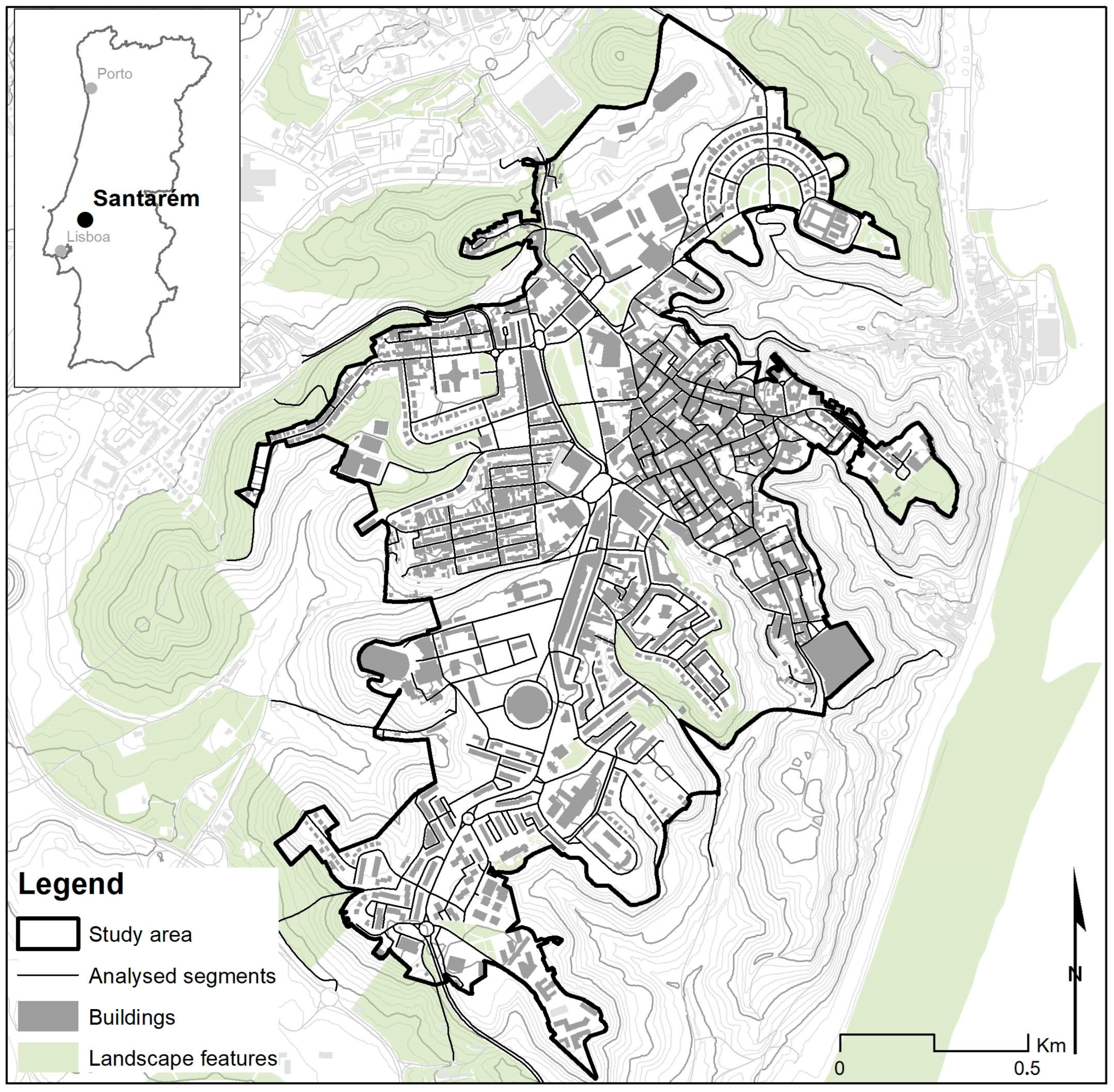
The methods applied aim to explore the relative contributions of connectivity measures and streetscape features in explaining walking trips. Section 1 describes the characteristics of the case study. Section 2 outlines the approach applied to evaluate the built environment characteristics at the street segment level. Section 3.3 explains the selection of the built environment indicators used in most of the walkability indexes developed in the literature, following the three Ds approach, but expanded with the evaluation of accessibility measures [44]. Section 4 describes the application of Purciel and Yin’s indicators to evaluate the streetscape features suggested by Ewing and Handy [11]. This chapter also includes the development of other indicators to measure these streetscape features. The last section describes the statistical methodology applied to explain walking trips for leisure and utilitarian purposes, considering the two types of approaches described previously.

3.1. Case Study

The context of this study is Santarém. This low-density, medium-sized Portuguese city (106.05 habitants/km2) [45] has been shaped by a particular topography (Figure 1). The historical center is located on a plateau that is at a higher altitude than the more recent urban development. Because of this key characteristic, the analysis was restricted to the city center in order to control for the impact of the topography on walking behavior. The medium-sized city context has complex challenges for active travel, related to the lack of public transport and uncomplicated car use (low traffic and parking availability). This is particularly important, because, in Portugal, small and medium-sized cities constitute a total of 121 cities, where 1.8 million inhabitants reside (17% of total population) [46]. The novelty of this context requires the testing of several indicators suggested in the literature. This justifies the testing of different density, diversity, design, and accessibility measures on the statistical modeling.

3.2. Data Collection

The scale of analysis is the 740 street segments defined by the topological rules used to create a network. The segments are located in the historical center of Santarém. These segments are a selection from a wider sample and were chosen because they are on a similar elevation plane, eliminating the influence of slope on walking trips. Moreover, they are the most central locations in Santarém. This study only uses quantitative and objective data, collected from different sources, including field collection.
Walking trip data were collected through a survey that was run in the context of the Integration of Land Use and Transportation in medium-sized cities (InLUT) project with the goal to evaluate the impact of the built environment on travel behavior [46]. The survey collects individuals’ socio-economic information, travel options (car ownership, public transport tickets, etc.), and daily trip diary.
Following the most relevant literature, data were aggregated per street segment rather than taking whole streets as units of evaluation [47]. Indicators were measured for each building, then averaged for each street segment. Setback distances were measured from the entrance of the building that was closest to the street segment. If there were no buildings on a segment, the endpoints and midpoints of the segments were used as base-points to evaluate 3D characteristics of street segments, rather than points closest to the buildings on each street.

3.3. Urban Structure the Three Ds Approach

Table 1 describes variables utilized in the evaluation of each dimension for the 740 street segments. Most data were calculated using ArcGIS toolboxes previously developed for the InLUT project, evaluated for a 500 m buffer from each building, then aggregated as described above. A distance of 500 m is typically used to define the bespoke neighborhood, which has the highest influence on daily activity, including walking [48]. Each dimension was captured by several indicators that were analyzed to evaluate their contribution to walking behavior in the specific context of Santarém, a medium-sized city. The indicators are described in detail below. This approach is the most common in the development of walkability indexes.

3.3.1. Density

Density, especially population density, influences the availability of transport infrastructures and the number of services and facilities [21,49]. The design of the city influences density values, not only in terms of population density, but also in terms of the number of buildings and activities. In that way, five types of density were evaluated, ranging from housing density (Dens1) to overall building density (Dens2) and the density of activities (Dens5).

3.3.2. Diversity

The density of population and activities can lead to a greater diversity of activities and services [21,49]. However, this may not be true for the medium-sized city context. To test this assumption, four diversity indicators are calculated based on detailed maps of building footprints and types of activity. The percentage of single-family buildings (Div1) describes the area occupied by detached houses. The percentage of residential buildings (Div2) captures all housing. Div3 captures the non-residential percentage of the area. Finally, the mixed-use indicator (Div4) evaluates the mixture of uses dedicated to different activities.

3.3.3. Design—Connectivity Measures

The structure design of the city defines the space distribution for the public and private space, and it has been measured by several connectivity measures [22]. Connectivity measures evaluate the road centerline network and include four indicators. The first is node density (Con1), which represents the density of nodes with more than three links within the 500 m network buffer. The second is the pedestrian shed ratio (Con2). This calculates the difference between the area defined by the 500 m circular buffer and the pedestrian catchment area (calculated with ArcGIS Network Analyst 10.6). Straightness (Con3) considers the distance that can be covered, as the crow flies, within the 500 m buffer. Mean link length (Con4) evaluates the length of street segments in the road network for all segments in the buffer.

3.3.4. Accessibility

Accessibility to activities is important for the individual’s daily routine. Moreover, public transport is an important destination as part of a trip sequence. All the trips start with a walking trip, and this is especially important for public transport trips. Following this assumption, accessibility to activities and public transport infrastructure were measured. The distance to the closest transit stop (Acc1) captures the distance in meters to the closest bus stop. Acc2 evaluates the daily public transport supply at the closest transit stop. Acc3 evaluates total public transport supply in the 500 m buffer. Acc4 captures the distance to the closest activity. Acc5 is the mean distance to the three closest activities. Acc6 is the number of activities within the 500 m meter buffer. Finally, Acc7 evaluates commercial continuity. This was assessed as the number of activities in the network, divided by the network distance.

3.3.5. Walking Trips

The dependent variable was the number of walking trips passing through streets in the study area. Walking trips were obtained through a travel survey of 1100 individuals (over 16 years old) living in Santarém. This survey captured walking trips, lasting over five minutes, made the previous working day (Monday and Friday were excluded, as trip patterns differ on these days, due to, for example, students returning home from studying outside the city). Interviews were taken door-to-door, and the survey was run in May 2013, thereby capturing mobility during a normal working/school week in mild weather. Interviewees reported a travel diary collecting the origin and destination of their trips and their motives; if a trip was combined with different purposes, like picking up groceries when returning home, this was recorded as two trips if it was more than five minutes long. Routes were estimated using ArcGIS Network Analyst 10.6, selecting the shortest option. Motives were subdivided into eight general groups, which were then classified as utilitarian or leisurely. Utilitarian trips included traveling to work or school and back, chauffeuring other family members, and traveling for meals because many individuals go home to have lunch. Outings for personal reasons were also considered as utilitarian trips. Leisure travel included shopping or recreation, along with outings for exercise, including running and walking. A total of 1788 trips were recorded. Most, 1344 (75%), were utilitarian, and only 444 (25%) were for leisure.

3.4. Urban Design Qualities

As described previously, urban street features are very important for walking because they influence the individual’s perception of the built environment’s attractiveness [15]. This paper does not evaluate individual perception, instead, it evaluates the streetscape feature that can shape this perception. The streetscape feature, important for individuals’ perceptions, was systematized in five dimensions by Ewing and Handy [11] and it includes imageability, enclosure, human scale, transparency, and complexity. The five dimensions proposed organize different streetscape features and several authors have developed methods and tools to evaluate it, including onsite collections, surveys, and, more recently, automated image classification.
The streetscape feature evaluation was built on the audit protocol assessment defined in the Ewing and Handy [11] study. The evaluation of the streetscape features was performed using the five dimensions of this protocol, and extends the work of Purciel et al. [38] and Yin [39], with some modifications that are described in the following sections. Table 2 systematizes the proposed indicators in Ewing and Handy’ work [11].

3.4.1. Number of Courtyards, Parks, and Plazas on the Block Face

Ewing and Handy [11] measured this indicator by counting the number of courtyards, plazas, or parks with a side that faced each unit block. In this paper, GIS data were used to calculate the total area covered by parks and green spaces (in m2) within the 500 m catchment area of each building and took the mean per street segment.

3.4.2. Proportion of Historic Building Frontages

Ewing and Handy [11] measured this indicator by dividing the total length of the historic building frontages (pre-World War II buildings) by the total length of each block face. The 2011 Census recorded the total number of pre-1945 buildings on a per-block basis; consequently, the mean number of buildings in neighboring blocks per building point was used, and then the mean for each street segment was calculated.

3.4.3. Number of Buildings with Identifiers

Ewing and Handy [11] define this measure as the number of buildings per block face with a sign indicating their use. In the present research, point-of-interest information provided by the city council (recorded in the InLUT project’s database) was used and uses that commonly require signage (e.g., stores, cafes, and bars) were identified, but other activities such as schools, vacant stores, and administrative functions were excluded. This method gave the number of buildings with identifiers for each street segment.

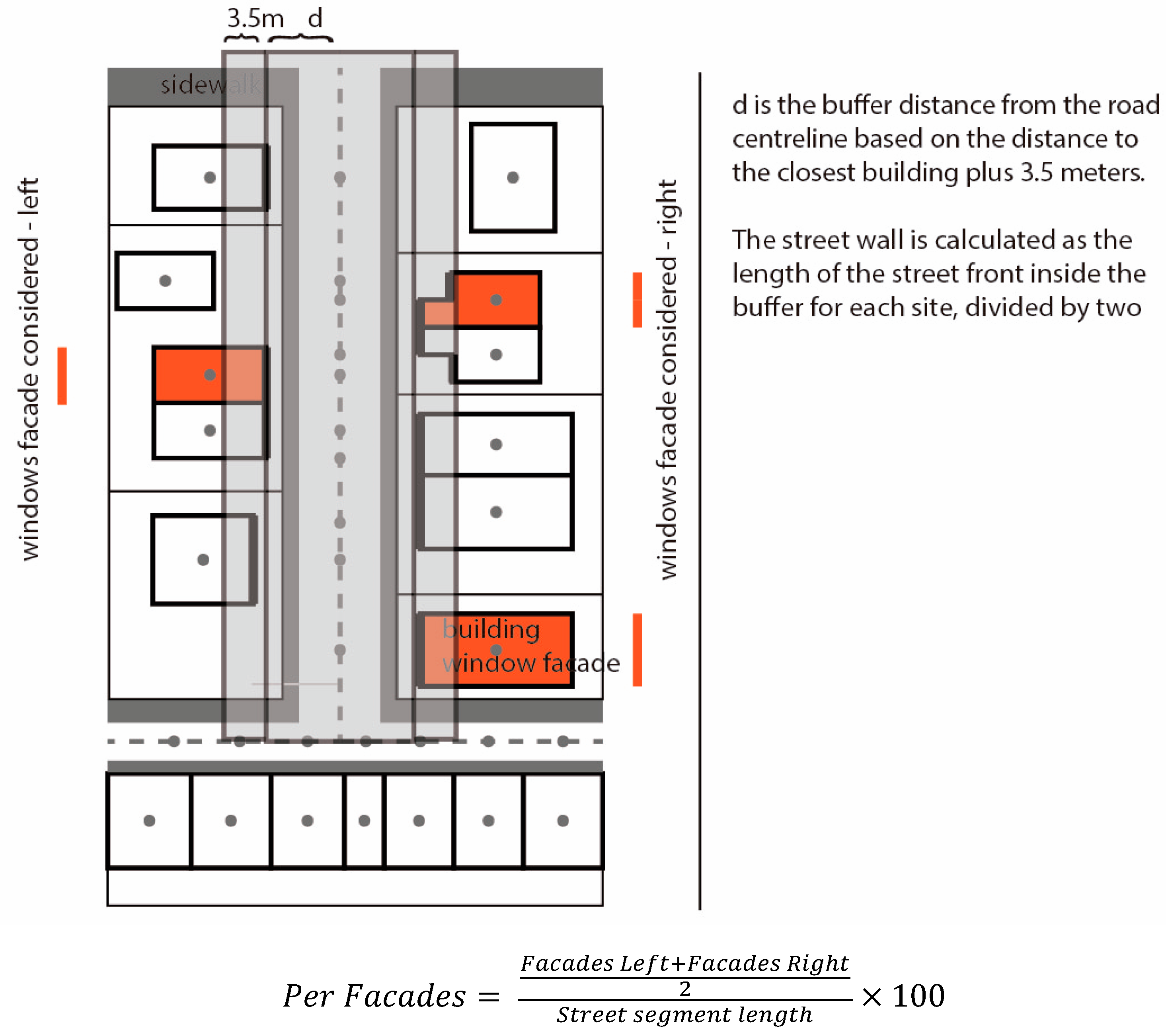
3.4.4. Proportion of Street Walls

Ewing and Handy [11] measured the proportion of street walls as the total length of block face taken up by buildings or other boundary elements, divided by the length of the block. The present paper used the length of building edges that touched the sidewalk and remained within a changing buffer for each street segment. An additional 3.5 m was added to the buffer (the distance from the closest building edge to the street segment), as this distance is considered to be the maximum within which visual and social interaction between the building’s inhabitants and people in the street is possible [37,50]. The result is the percentage of each segment adjacent to boundary elements (see Figure 2).

3.4.5. Mean Building Height

Ewing and Handy [11] defined this measure as the approximate height of each building, calculated by multiplying the number of floors per building by the mean height of each block face. For the present paper, building height was calculated by multiplying the number of floors by 3.5, but did not weigh each building’s height value based on its facade length. The value for the street segment was calculated as the mean height of all buildings in the segment.

3.4.6. Facades with Windows to Total Facades Proportion

Ewing and Handy [11] made a visual estimate of the percentage of facades with windows compared to the total facade area on the ground floor of buildings per block face. Like buildings with an identifier, buildings that were likely to have facades were determined. Their total length was divided by the total of all building facade lengths per street segment. The result is the percentage of the street segment occupied by windows (see Figure 3).

3.4.7. Total Number of Buildings per Block Face

The number of buildings with direct access to each street segment was computed.

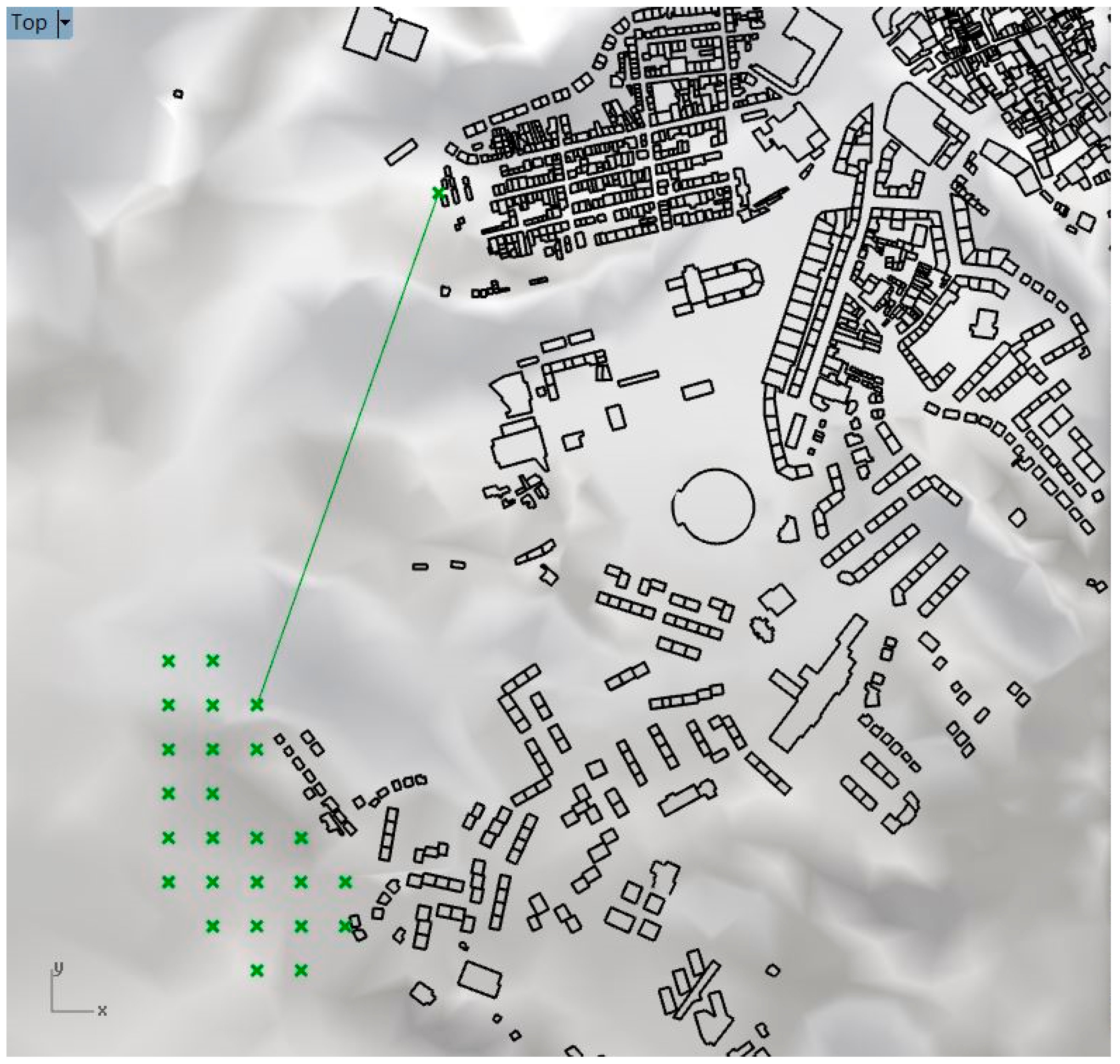
3.4.8. Visibility of Major Landscape Features

This measure requires counting all landscape features when walking along the street; examples include mountains, water bodies, or greenery. For this measure, a 3D digital model of the city was used. Starting from building access points from each street segment, eye-level points were created by elevating them to 1.5 m above ground. Then, a ray-casting method was used to send rays to grids of points on landscape elements such as green areas and the Tagus river. Based on the unobstructed rays reaching each landscape element, the number of landscape elements visible from each point were computed. Finally, the mean values for all points was calculated per street segment (Figure 4).

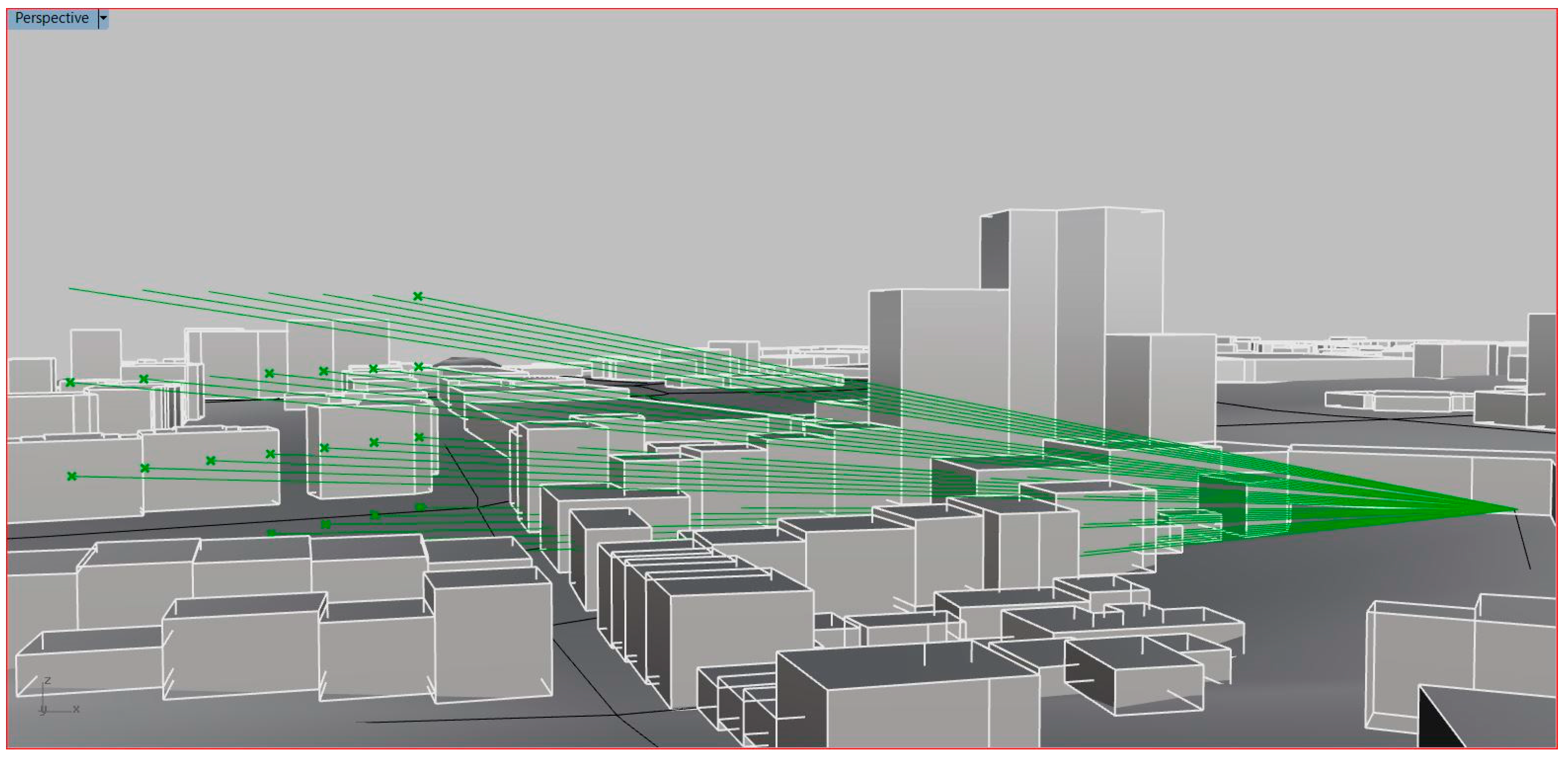
3.4.9. Proportion of Visible Sky

Ewing and Handy’s [11] method requires the auditor to estimate the percentage of visible sky in three directions from several points along a block face in their frame of view. Again, utilizing the 3D city model, a view frame in four directions was created that was 168 m from points of view that were 1.5 m above ground to simulate eye level for each building point, following the criteria of Purciel et al. [38]. The next step was casting rays to a grid of points in the view frame and calculating the percentage of rays that were not interrupted by buildings or topography (see Figure 5).

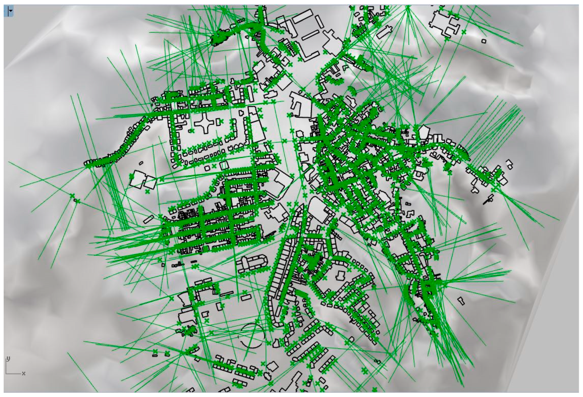
3.4.10. Number of Long Sightlines

In Ewing and Handy’s method [11], the auditor is directed to look in three directions from several points along a block face, and count the instances where the sightline is uninterrupted. Using a 3D model, 300 m rays were sent out in four directions from the building base points at 1.5 m above ground level and instances were counted where they were not interrupted by buildings or topography (see Figure 6).

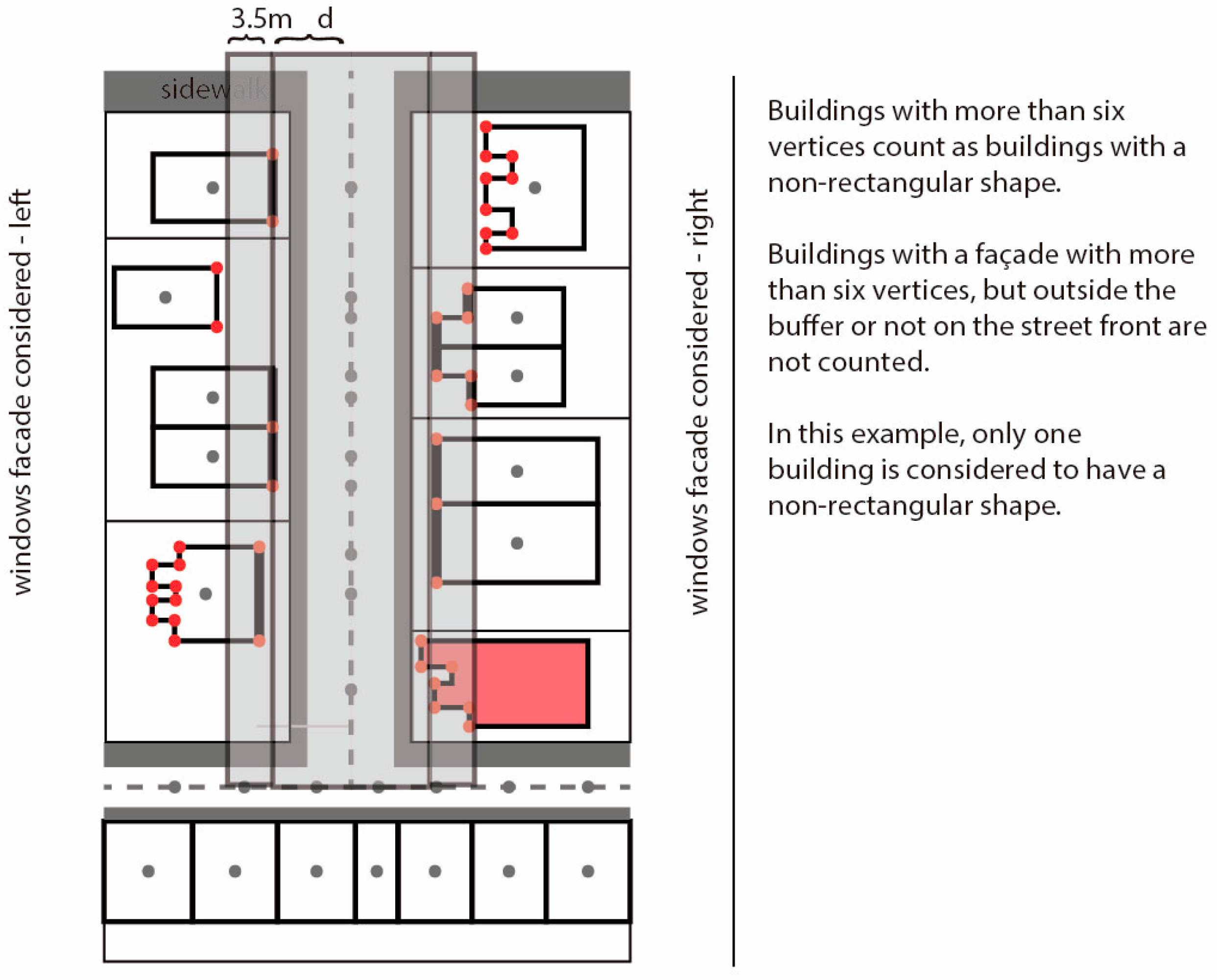
3.4.11. Number of Buildings with Non-Rectangular Shapes

The building footprints were used to capture non-rectangular buildings. Furthermore, it was assumed that buildings with more than six vertices on the facade had a non-rectangular shape. The present paper approach takes into account the fact that facades of one building can be different on different streets (see Figure 7).

3.5. Statistical Analyses

Descriptive statistics for all considered indicators and dimensions are presented in Table 1. Motives for walking were tested using a multiple regression analysis based on models of utilitarian and leisure trips. The regression models to explain the walking trips were tested with three models: one using connectivity measures, another for using streetscape feature measures by GIS and 3D indicators, and a third model that combined all indicators. Multicollinearity was evaluated with the variance influence factor (VIF), adopting the assumption that values above 10 are impossible to use [51], most variables have a VIF value lower than 5.

4. Results

4.1. All Trips

Table 3 presents the results for the three multiple linear regressions for all walking trips (1788) considering the three models.
The first model, using connectivity measures, explains 55% of the variance (adjusted R2 = 0.549). The density, diversity, and connectivity dimensions have variables that are significant at p < 0.001. These results confirm the importance of the thee Ds’ dimensions (density, diversity, and design) and accessibility to explain walking behavior, with statistically significant results for each dimension.
The second model, which was based on streetscape features, explained 48% of the variance (adjusted R2 = 0.483), which is 7% less than the first model. The streetscape features diversity and accessibility to public transport are found to be important indicators to explain walking trips.
The third model evaluated both connectivity and streetscape features. This model explained 60% of the variance (adjusted R2 = 0.599), which is 5% higher than model one (the connectivity model) and 12% higher than model two (streetscape features). The joint model shows that all the considered dimensions have indicators significant enough to explain walking trips.

4.2. Utilitarian Trips

The results for the three models of utilitarian trips (1344), which make up 75% of the trips, are presented in Table 4. The adjusted R2 values are similar to the results for all the trips. However, they are lower in the third model. Similarly, these values are lower in model two compared to the same model for all the trips. These changes suggest that streetscape features are less relevant in explaining utilitarian trips.
In model one, using connectivity measures, the coefficient values increase for the density indicators. In the diversity dimension, the indicator remains statistically significant, but values decrease compared to all the trips. As for connectivity measures, the behavior is very similar to all the trips. In the accessibility dimension, the statistically significant variables are the same as for the overall sample.
In model two, using streetscape features, the housing density is statistically significant (Div 1, β = 0.137, p < 0.001). The same is true for diversity, concerning the percentage of single-family buildings (Div 1, β = 0.191, p < 0.001) in the diversity dimension. The results for the accessibility dimension are similar to the results for the overall sample.
In model three, for the connectivity and streetscape features, the density and diversity variables display a similar behavior. For the connectivity measures, the results are similar to those for the overall sample. As for the streetscape features, the pattern of results is similar to the overall sample. The major difference is the statistical significance of the mean building height (Dsg8, β = 0.115, p < 0.001). Finally, in the accessibility dimension, the values are very similar to the results for all the trips.

4.3. Leisure Trips

The results of the models for the leisure trips (444, 25%) are illustrated in Table 5. The explanatory powers of the three models are quite different. The adjusted R2 is lower than for all the trips and utilitarian trips.
In model one, using connectivity measures, the diversity and the connectivity values have a similar pattern with all the trips. In the density dimension, the services and retail gross floor area ratio lose statistical significance when comparing with the utilitarian trips. The accessibility dimension varies the most—in both the overall sample and utilitarian trips—with the reduction in coefficient values.
In the case of model two’s streetscape features, unlike the overall sample, the different density indicators are statistically significant. In the diversity dimension, the urban complexity (Div1) remains statistically significant. Although the values for the accessibility dimension are similar to those for model one, they are clearly different from the same model for all the trips and utilitarian trips. Here, the coefficients are lower, and only the distance to the closest transit stop is statistically significant (β = −0.424, p < 0.001).
In model three, using connectivity and streetscape features, the results for the density, diversity, and connectivity dimensions are similar to the entire sample. Within the accessibility dimension, the distance to the closest transit stop remains the only statistically significant variable (Acc1) (β = −0.339, p < 0.001).

5. Discussion

The results show that the models using the connectivity indicators have a slightly higher adjusted R2 than the models that use the streetscape indicators to explain the utilitarian walking trips and the walking trips in general. On other hand, the models combining the connectivity and streetscape indicators have a higher adjusted R2 for the different trip purposes. Nevertheless, the different indicators have different importances considering the trip purposes.
Looking in detail at the differences between the impact of the indicators in relation to the trip motives, even though the overall pattern is similar, a slight difference can be identified with respect to the leisure trips. Here, the coefficient values of the density indicator decline, and the density of the services loses statistical significance. Moreover, the accessibility measures become less important. The results for the leisure trips highlight the reduced importance of the service and retail density. Access to public transport is important for utilitarian trips, but less important for leisure trips.
Analyzing the three models and the two trip motives, the connectivity measures were found to be the most stable. The accessibility shows the greatest variance and is less significant with respect to leisure trips. The streetscape model has the lowest explanation power of the models when comparing with the connectivity measures and the combined indicators.
The results reinforce the significance of the connectivity measures in explaining walking [52]. Better connectivity increases walking route options, and expands the building frontages that can provide street-level activities [25,53]. Nevertheless, the streetscape features are crucial for defining the attractiveness of the street-level activities. Changing the streetscape is more feasible than altering the urban form, and it can have an impact on street appeal, thus increasing the number of people who walk [15,16,54]. The evaluation of streetscape features and their impact on urban design qualities helps us to better understand the built environment, and can explain a significant amount of the variance in walking behavior. Moreover, streetscape features are significantly different from connectivity measures, which raises the question of the validity of connectivity measures as a proxy for design qualities when evaluating walkability conditions. Finally, the streetscape can improve the quality of the urban environment and the walking experience, but appears to have a lesser influence on walking in general [40].
The results suggest that streetscape features have a lesser influence on walking in general; however, their contribution to the quality of the urban environment has an impact on individuals’ walking experiences [13,14,15,16]. This positive or negative experience defines individual travel satisfaction, which contributes to the creation of captive users in different travel modes [55,56]. The satisfaction of the walking experience contributes to the maintenance of travel habits, especially for walking. Streetscape features play an important role in an individual’s perception of built environments. The improvement of this streetscape’s features can contribute to a better perception of the built environment by creating higher street attractiveness. Nevertheless, these perceptions will depend on the individual’s personal context, which is defined by their past and personal conditions [13].
The higher importance of the connectivity measures to explain walking trips supports the importance of use connectivity measures for walkability indicators. This also reinforces the importance of placing more importance on connectivity measures to create these walkability indexes [28]. However, the necessity of evaluating these streetscapes to explain walking behavior is reinforced by the higher explanation power of the model with the two types of indicators. This paper fulfils the gap in the research on walking behavior, evaluating the three dimensions described by the Behavioral Model of the Environment [18,19], considering the estimated origin, destination, and the route characteristics.
The results make an important contribution to the research by providing tools and methods to evaluate the streetscape features that influence individuals’ perceptions. The application of the suggested tools can be made at different scales of analysis, identifying environments that are more human- and walking-friendly and that support more sustainable, and generally healthier, modes of transportation. The tools and indicators can be used and tested in the development of new walkability indicators, including not only the network topological aspect but also the street design characteristics that have been shown to be important in influencing walking behavior. This evaluation can be used to define a strategic approach to promote the use of sustainable modes of transportation and individuals’ wellbeing where there are worse built environment conditions, which present a higher risk of deprivation [57].
The proposed indicators and methods have a few limitations. First, these indicators do not capture data on individuals’ perceptions for walking trips or travel satisfaction. Secondly, the indicators used do not evaluate aspects such as safety and security used in most of the audit measures found in the literature and that are important for specific groups and contexts [14,58]. Thirdly, the walking route data utilized are estimates based on the shortest routes between origin and destination points on the street network, rather than actual routes. This limitation can lead to a bias overestimating the importance of the connectivity measures. Nevertheless, the models evaluate the contribution of the real street segment characteristics of the origins and destinations of trips. Further research on the dataset could involve an exploration of the relative contribution of street segments of origins and destinations as suggested by the Behavioral Model of the Environment [18,19]. The approach employed to assess walking trips simplifies the complexity of daily routines by treating each origin and destination as a separate trip. However, the choice of transportation mode is determined by all the trips taken throughout the day. Thus, a single trip can significantly impact the decision for all subsequent trips within the day, such as dropping children off at school.
Nevertheless, this study offers some insights for further research. For example, future work could evaluate streetscape characteristics’ capacity to predict perceptions, which can be tested with new virtual reality tools [59]. The results point to the importance of the accessibility of public transport in increasing the number of people walking; however, the quality of the trip experience was not evaluated. This paper also provides insight into the means to improve the walkability indices that are used extensively in the literature. Particularly, it suggests the introduction of new indicators that can be used at different-scale evaluations.

6. Conclusions

In conclusion, this paper presents a new approach for the improvement of methods and indicators used in the evaluation of the built environment conditions that influence walking behavior. Firstly, it challenges the applicability of the theoretical model of Ewing and Handy [11] in a low-density and urban Portuguese context. Secondly, through a case study, it is proposed that connectivity measures have a greater explanatory power than models based on evaluating streetscape features. However, the joint evaluation of the connectivity and streetscape performs best.
In this paper, the importance of accessibility for walking is highlighted, especially for utilitarian trips. The results confirm the significance of the urban form assessed by connectivity measures, which are used in most of the walkability literature to explain trips with different motives. Nevertheless, the introduction of streetscape features into an evaluation can help in further explaining walking. The results emphasize the importance of the streetscape characteristics’ influence on a range of walking activities; a finding particularly valuable given that it is easier to improve smaller-scale built environment features than changing the urban form.
The new measures enable the evaluation of indicators at different levels of analysis and without the requirement of onsite audits. Such approaches become more relevant as more data regarding streetscape features relevant for measuring the walkability of built environments become available for an expanding range of geographies every day. Moreover, the increasing adoption of automated and AI-supported methods to measure and evaluate built environment characteristics provides new tools and data to understand the impact of built environment characteristics on individuals’ routines. This new information can be used to evaluate the results of urban interventions and planning policies. Future work could investigate the contribution of streetscape features to different walkability indices, using the newly proposed indicators. There is research yet to be performed for validating walkability measures based on perceptual indicators such as safety, comfort, and attraction, looking at walking as both a mode of travel and a recreational activity. The proposed indicators can be used in the development and calibration of new walkability indexes developed for European contexts, suggesting the great potential of the indicators combined in these indexes.

Author Contributions

Conceptualization, M.F.P. and D.S.V.; methodology, M.F.P. and D.S.V.; writing—original draft preparation, M.F.P.; writing—M.F.P.; visualization, M.F.P.; supervision, D.S.V. and P.S.; funding acquisition, D.S.V. All authors have read and agreed to the published version of the manuscript.

Funding

This research was funded by Fundação para a Ciência e a Tecnologia, I.P. (FCT), under the Strategic Project with the references grant UIDB/04008/2020 and UIDP/04008/2020. This research is part of PhD project funding with the code SFRH/BD/110568/2015. Paula Santana is a member of the CEGOT-UC, funded by national funds, through the FCT, under the reference UIDB/04084/2020.

Data Availability Statement

The raw data supporting the conclusions of this article will be made available by the authors on request.

Acknowledgments

The authors would like to acknowledge all the research support from the Research Centre for Architecture, Urbanism and Design (CIAUD). The authors would like to thank Elif Ensari Sucuoglu (ORCID—0000-0003-0451-2217) for the help in calculating 3D model indicators.

Conflicts of Interest

The authors declare no conflicts of interest.

References

  1. Blitz, A.; Lanzendorf, M. Mobility Design as a Means of Promoting Non-Motorised Travel Behaviour? A Literature Review of Concepts and Findings on Design Functions. J. Transp. Geogr. 2020, 87, 102778. [Google Scholar] [CrossRef]
  2. Næss, P. Urban Form and Travel Behavior: Experience from a Nordic Context. J. Transp. Land Use 2012, 5, 21–45. [Google Scholar] [CrossRef]
  3. Ewing, R.; Cervero, R. Travel and the Built Environment: A Synthesis. J. Am. Plan. Assoc. 2010, 76, 265–294. [Google Scholar] [CrossRef]
  4. Frumkin, H.; Frank, L.D.; Jackson, R. Urban Sprawl and Public Health: Designing, Planning, and Building for Healthy Communities; Island Press: London, UK, 2004; ISBN 9781597266314. [Google Scholar]
  5. Barton, H. City of Well-Being; Routledge: New York, NY, USA, 2017; ISBN 978-0-415-63932-3. [Google Scholar]
  6. Pereira, M.F.; Almendra, R.; Vale, D.S.; Santana, P. The Relationship between Built Environment and Health in the Lisbon Metropolitan Area—Can Walkability Explain Diabetes’ Hospital Admissions? J. Transp. Health 2020, 18, 100893. [Google Scholar] [CrossRef]
  7. UN—Habitat. Habitat III New Urban Agenda: Quito Declaration on Sustainable Cities and Human Settlements for All. In Proceedings of the United Nations Conference on Houssing and Sustainable Urban Development, Quito, Ecuador, 17–20 October 2016; p. 24. [Google Scholar]
  8. Patel, V.; Saxena, S.; Lund, C.; Thornicroft, G.; Baingana, F.; Bolton, P.; Chisholm, D.; Collins, P.Y.; Cooper, J.L.; Eaton, J.; et al. The Lancet Commission on Global Mental Health and Sustainable Development. Lancet 2018, 392, 1553–1598. [Google Scholar] [CrossRef]
  9. Wang, H.; Yang, Y. Neighbourhood Walkability: A Review and Bibliometric Analysis. Cities 2019, 93, 43–61. [Google Scholar] [CrossRef]
  10. Frank, L.D.; Sallis, J.F.; Conway, T.L.; Chapman, J.E.; Saelens, B.E.; Bachman, W. Many Pathways from Land Use to Health: Associations between Neighborhood Walkability and Active Transportation, Body Mass Index, and Air Quality. J. Am. Plan. Assoc. 2006, 72, 75–87. [Google Scholar] [CrossRef]
  11. Ewing, R.; Handy, S. Measuring the Unmeasurable: Urban Design Qualities Related to Walkability. J. Urban Des. 2009, 14, 65–84. [Google Scholar] [CrossRef]
  12. Saelens, B.E.; Handy, S.L. Built Environment Correlates of Walking: A Review. Med. Sci. Sport. Exerc. 2008, 40, 550–566. [Google Scholar] [CrossRef]
  13. Hillnhütter, H. Stimulating Urban Walking Environments—Can We Measure the Effect? Environ. Plan. B Urban Anal. City Sci. 2022, 49, 275–289. [Google Scholar] [CrossRef]
  14. Arellana, J.; Saltarín, M.; Larrañaga, A.M.; Alvarez, V.; Henao, C.A. Urban Walkability Considering Pedestrians’ Perceptions of the Built Environment: A 10-Year Review and a Case Study in a Medium-Sized City in Latin America. Transp. Rev. 2019, 40, 183–203. [Google Scholar] [CrossRef]
  15. Kim, S.; Park, S.; Lee, J.S. Meso- or Micro-Scale? Environmental Factors Influencing Pedestrian Satisfaction. Transp. Res. Part D Transp. Environ. 2014, 30, 10–20. [Google Scholar] [CrossRef]
  16. Steinmetz-Wood, M.; El-Geneidy, A.; Ross, N.A. Moving to Policy-Amenable Options for Built Environment Research: The Role of Micro-Scale Neighborhood Environment in Promoting Walking. Health Place 2020, 66, 102462. [Google Scholar] [CrossRef] [PubMed]
  17. Kang, B.; Moudon, A.V.; Hurvitz, P.M.; Saelens, B.E. Differences in Behavior, Time, Location, and Built Environment between Objectively Measured Utilitarian and Recreational Walking. Transp. Res. Part D Transp. Environ. 2017, 57, 185–194. [Google Scholar] [CrossRef] [PubMed]
  18. Lee, C.; Moudon, A.V. Physical Activity and Environment Research in the Health Field: Implications for Urban and Transportation Planning Practice and Research. J. Plan. Lit. 2004, 19, 147–181. [Google Scholar] [CrossRef]
  19. Moudon, A.V.; Lee, C. Walking and Bicycling: An Evaluation of Environmental Audit Instruments. Am. J. Health Promot. 2003, 18, 21–37. [Google Scholar] [CrossRef] [PubMed]
  20. Frank, L.D.; Schmid, T.L.; Sallis, J.F.; Chapman, J.; Saelens, B.E. Linking Objectively Measured Physical Activity with Objectively Measured Urban Form: Findings from SMARTRAQ. Am. J. Prev. Med. 2005, 28, 117–125. [Google Scholar] [CrossRef]
  21. Rynning, M.K. Towards a Zero-Emission Urban Mobility Urban Design as a Mitigation Strategy, Harmonizing Insights from Research and Practice (researchgate.net). Ph.D. Thesis, National Institute of Applied Sciences of Toulouse, Toulouse, France, 2018. [Google Scholar]
  22. Vale, D.S.; Saraiva, M.; Pereira, M. Active Accessibility: A Review of Operational Measures of Walking and Cycling Accessibility. J. Transp. Land Use 2016, 9, 209–235. [Google Scholar] [CrossRef]
  23. Fonseca, F.; Ribeiro, P.J.G.; Conticelli, E.; Jabbari, M.; Tondelli, S.; Ramos, R.A.R.; Fonseca, F.; Ribeiro, P.J.G.; Conticelli, E.; Jabbari, M.; et al. Built Environment Attributes and Their Influence on Walkability. Int. J. Sustain. Transp. 2021, 16, 660–679. [Google Scholar] [CrossRef]
  24. Boeing, G. Measuring the Complexity of Urban Form and Design. Urban Des. Int. 2018, 23, 281–292. [Google Scholar] [CrossRef]
  25. Pafka, E.; Dovey, K. Permeability and Interface Catchment: Measuring and Mapping Walkable Access. J. Urban. 2017, 10, 150–162. [Google Scholar] [CrossRef]
  26. Ellis, G.; Hunter, R.; Tully, M.A.; Donnelly, M.; Kelleher, L.; Kee, F. Connectivity and Physical Activity: Using Footpath Networks to Measure the Walkability of Built Environments. Environ. Plan. B Plan. Des. 2016, 43, 130–151. [Google Scholar] [CrossRef]
  27. Ozbil, A.; Gurleyen, T.; Yesiltepe, D.; Zunbuloglu, E. Comparative Associations of Street Network Design, Streetscape Attributes and Land-Use Characteristics on Pedestrian Flows in Peripheral Neighbourhoods. Int. J. Environ. Res. Public Health 2019, 16, 1846. [Google Scholar] [CrossRef]
  28. Frank, L.D.; Sallis, J.F.; Saelens, B.E.; Leary, L.; Cain, K.; Conway, T.L.; Hess, P.M.; Cain, L.; Conway, T.L.; Hess, P.M. The Development of a Walkability Index: Application to the Neighborhood Quality of Life Study. Br. J. Sports Med. 2010, 44, 924–933. [Google Scholar] [CrossRef] [PubMed]
  29. Grasser, G.; van Dyck, D.; Titze, S.; Stronegger, W.J. A European Perspective on GIS-Based Walkability and Active Modes of Transport. Eur. J. Public Health 2017, 27, 145–151. [Google Scholar] [CrossRef] [PubMed]
  30. Ewing, R.; Clemente, O. Measuring Urban Design: Metrics for Liveable Places; Island Press: Washington, DC, USA, 2013; ISBN 9781610911931. [Google Scholar]
  31. Millstein, R.A.; Cain, K.L.; Sallis, J.F.; Conway, T.L.; Geremia, C.M.; Frank, L.D.; Chapman, J.; Van Dyck, D.; Dipzinski, L.R.; Kerr, J.; et al. Development, Scoring, and Reliability of the Microscale Audit of Pedestrian Streetscapes (MAPS). BMC Public Health 2013, 13, 403. [Google Scholar] [CrossRef] [PubMed]
  32. Su, S.; Zhou, H.; Xu, M.; Ru, H.; Wang, W.; Weng, M. Auditing Street Walkability and Associated Social Inequalities for Planning Implications. J. Transp. Geogr. 2019, 74, 62–76. [Google Scholar] [CrossRef]
  33. Cain, K.L.; Gavand, K.A.; Conway, T.L.; Geremia, C.M.; Millstein, R.A.; Frank, L.D.; Saelens, B.E.; Adams, M.A.; Glanz, K.; King, A.C.; et al. Developing and Validating an Abbreviated Version of the Microscale Audit for Pedestrian Streetscapes (MAPS-Abbreviated). J. Transp. Health 2017, 5, 84–96. [Google Scholar] [CrossRef] [PubMed]
  34. Kyttä, M.; Broberg, A.; Haybatollahi, M.; Schmidt-Thomé, K. Urban Happiness: Context-Sensitive Study of the Social Sustainability of Urban Settings. Environ. Plan. B Plan. Des. 2016, 43, 34–57. [Google Scholar] [CrossRef]
  35. Stefansdottir, H. The Role of Urban Atmosphere for Non-Work Activity Locations. J. Urban Des. 2018, 23, 319–335. [Google Scholar] [CrossRef]
  36. Jiao, J.; Drewnowski, A.; Moudon, A.V.; Aggarwal, A.; Oppert, J.-M.; Charreire, H.; Chaix, B. The Impact of Area Residential Property Values on Self-Rated Health: A Cross-Sectional Comparative Study of Seattle and Paris. Prev. Med. Rep. 2016, 4, 68–74. [Google Scholar] [CrossRef] [PubMed]
  37. Gehl, J. Life between Buildings—Using Public Space, 6th ed.; Island Press: London, UK, 2011; ISBN 9781597268271. [Google Scholar]
  38. Purciel, M.; Neckerman, K.M.; Lovasi, G.S.; Quinn, J.W.; Weiss, C.; Bader, M.D.M.; Ewing, R.; Rundle, A. Creating and Validating GIS Measures of Urban Design for Health Research. J. Environ. Psychol. 2009, 29, 457–466. [Google Scholar] [CrossRef] [PubMed]
  39. Yin, L. Street Level Urban Design Qualities for Walkability: Combining 2D and 3D GIS Measures. Comput. Environ. Urban Syst. 2017, 64, 288–296. [Google Scholar] [CrossRef]
  40. Cambra, P.; Moura, F. How Does Walkability Change Relate to Walking Behavior Change? Effects of a Street Improvement in Pedestrian Volumes and Walking Experience. J. Transp. Health 2020, 16, 100797. [Google Scholar] [CrossRef]
  41. Van Dyck, D.; Cerin, E.; Conway, T.L.; De Bourdeaudhuij, I.; Owen, N.; Kerr, J.; Cardon, G.; Frank, L.D.; Saelens, B.E.; Sallis, J.F. Perceived Neighborhood Environmental Attributes Associated with Adults’ Leisure-Time Physical Activity: Findings from Belgium, Australia and the USA. Health Place 2013, 19, 59–68. [Google Scholar] [CrossRef] [PubMed]
  42. Yang, Y.; Diez-Roux, A.V. Walking Distance by Trip Purpose and Population Subgroups. Am. J. Prev. Med. 2012, 43, 11–19. [Google Scholar] [CrossRef] [PubMed]
  43. Giles-Corti, B.; Timperio, A.; Bull, F.; Pikora, T. Understanding Physical Activity Environmental Correlates: Increased Specificity for Ecological Models. Exerc. Sport Sci. Rev. 2005, 33, 175–181. [Google Scholar] [CrossRef] [PubMed]
  44. Vale, D.S.; Pereira, M. Influence on Pedestrian Commuting Behavior of the Built Environment Surrounding Destinations: A Structural Equations Modeling Approach. Int. J. Sustain. Transp. 2016, 10, 730–741. [Google Scholar] [CrossRef]
  45. PORDATA. PORData Estatisticas Sobre Portugal e a Europa. Available online: https://www.pordata.pt/Municipios/Densidade+populacional-452 (accessed on 7 September 2022).
  46. Vale, D.S.; Rosa, M.; Pereira, M.F.; Saraiva, M.; Bento, R.; Alves, R.; Marshall, S. Integração de Usos Do Solo e Transportes Em Cidades de Média Dimensão; Alves, R.A., Vale, D.S., Eds.; Bibliografia National Portuguesa: Lisboa, Portugal, 2018; ISBN 978-972-24-1863-8. [Google Scholar]
  47. Taleai, M.; Taheri Amiri, E. Spatial Multi-Criteria and Multi-Scale Evaluation of Walkability Potential at Street Segment Level: A Case Study of Tehran. Sustain. Cities Soc. 2017, 31, 37–50. [Google Scholar] [CrossRef]
  48. Learnihan, V.; Van Niel, K.P.; Giles-Corti, B.; Knuiman, M. Effect of Scale on the Links between Walking and Urban Design. Geogr. Res. 2011, 49, 183–191. [Google Scholar] [CrossRef]
  49. Forsyth, A.; Oakes, J.M.; Schmitz, K.H.; Hearst, M. Does Residential Density Increase Walking and Other Physical Activity? Urban Stud. 2007, 44, 679–697. [Google Scholar] [CrossRef]
  50. Gehl, J.; Svarre, B. How to Study Public Life; Island Press: London, UK, 2013. [Google Scholar]
  51. Marôco, J. Análise Estatística Com o PASW Statistics (Ex-SPSS); Report Number; Lda: Pêro Pinheiro, Portugal, 2010; ISBN 978-989-96763-0-5. [Google Scholar]
  52. Frank, L.D.; Engelke, P.O. The Built Environment and Human Activity Patterns: Exploring the Impacts of Urban Form on Public Health. J. Plan. Lit. 2001, 16, 202–218. [Google Scholar] [CrossRef]
  53. Sevtsuk, A.; Kalvo, R.; Ekmekci, O. Pedestrian Accessibility in Grid Layouts: The Role of Block, Plot and Street Dimensions. Urban Morphol. 2016, 20, 89–106. [Google Scholar] [CrossRef]
  54. Erturan, A.; van der Spek, S.C. Walkability Analyses of Delft City Centre by Go-Along Walks and Testing of Different Design Scenarios for a More Walkable Environment. J. Urban Des. 2022, 27, 287–309. [Google Scholar] [CrossRef]
  55. De Vos, J.; Schwanen, T.; Van Acker, V.; Witlox, F. How Satisfying Is the Scale for Travel Satisfaction? Transp. Res. Part F Traffic Psychol. Behav. 2015, 29, 121–130. [Google Scholar] [CrossRef]
  56. Mouratidis, K.; Ettema, D.; Næss, P. Urban Form, Travel Behavior, and Travel Satisfaction. Transp. Res. Part A Policy Pract. 2019, 129, 306–320. [Google Scholar] [CrossRef]
  57. Pereira, M.F.; Vale, D.S.; Santana, P. Is Walkability Equitably Distributed across Socio-Economic Groups? —A Spatial Analysis for Lisbon Metropolitan Area. J. Transp. Geogr. 2023, 106, 103491. [Google Scholar] [CrossRef]
  58. Appleyard, B. Livable Streets for Schoolchildren: A Human-Centred Understanding of the Cognitive Benefits of Safe Routes to School. J. Urban Des. 2022, 27, 692–716. [Google Scholar] [CrossRef]
  59. Nakamura, K. Experimental Analysis of Walkability Evaluation Using Virtual Reality Application. Environ. Plan. B Urban Anal. City Sci. 2021, 48, 2481–2496. [Google Scholar] [CrossRef]
Figure 1. Santarém, Portugal.
Urbansci 08 00024 g001
Figure 2. Proportion of street wall calculation (authors).
Urbansci 08 00024 g002
Figure 3. Calculation of the proportion of building facades (authors).
Urbansci 08 00024 g003
Figure 4. Model to calculate the visibility of major landscape features. The ray-casting lines in green.
Urbansci 08 00024 g004
Figure 5. Model to calculate the proportion of visible sky. In green color, the casting rays to a grid of points in the view frame.
Urbansci 08 00024 g005
Figure 6. Number of long sightlines. In green color, the 300 m rays in four directions from building base points at 1.5 m above ground level.
Urbansci 08 00024 g006
Figure 7. Method to identify non-rectangular buildings (authors).
Urbansci 08 00024 g007
Table 1. Variables and descriptive statistics.
Street Segments Descriptive Statistics (N = 740)
VariableDescriptionSourceYearUnitMinMaxMeanSkewKurtosis
Density
Dens1Housing density (Dwellings per ha)(1)2013number1.3876.6534.390.10−0.19
Dens2Building Density (Buildings per ha)(1)2013number1.6029.7313.01−0.07−1.38
Dens3Gross Floor Area Ratio (Index)(1)2013index0.081.640.84−0.27−0.55
Dens4Housing gross floor area ratio (Index)(1)2013index0.030.930.460.21−0.50
Dens5Services and retail gross floor area ratio (Index)(1)2013index0.000.790.380.09−1.33
Diversity
Div1Percentage of single family buildings (% of buildings)(1)2013%4.4458.4123.031.502.87
Div2Percentage of residential dwellings (% of dwellings)(1)2013%43.6195.5470.75−0.15−1.35
Div3Percentage of area occupied by activities (% of area of each activity)(1)2013%0.0417.837.570.37−1.26
Div4Urban complexity (Index ≥ 0)(1)2013index1.812.652.45−0.825.88
DesignConnectivity
Con1Node density (Nodes per ha)(1)2013number0.264.152.37−0.11−0.77
Con2Pedestrian shed ratio (Index ]0–1] )(1)2013index0.120.670.44−0.53−0.28
Con3Straightness (ratio)(1)2013ratio0.540.960.75−0.511.24
Con4Average link length (meters)(1)2013meters33.8199.0146.161.402.52
DesignStreetscape features
Dsg1Mean of square meter of green spaces for each building in segment(1)2013meters0.0026,866.028742.090.79−0.32
Dsg2Mean of long sight line views of major landscape for segment(1)2013number0.003.000.381.713.18
Dsg3Mean of buildings constructed before 1945(2)2011%0.00100.0027.390.85−0.51
Dsg4 *Sum of the number of buildings with identifier in each segment(1)2013number0.007.750.941.433.97
Dsg5Percentage of rays not interrupted by buildings of topography (Proportion sky)(1)2013 %0.001.000.160.940.88
Dsg6Proportion of segment surrounded by walls(1)2013%0.00100.0075.28−1.09−0.22
Dsg7Average of uninterrupted view to major landscape(1)2013number0.006.000.831.793.44
Dsg8Mean building height for each segment(1)2013meters0.0031.5010.501.401.19
Dsg9Proportion of segment occupied by activities with windows(1)2013%0.00100.0023.861.280.44
Dsg10 *Total of buildings in each segment(1)2013number1.006.321.961.553.85
Dsg11Number of building with non–rectangular shape(1)2013number0.007.001.091.181.19
Acessibility
Acc1Distance to the closest transit stop (meters)(1)2013meters10.511085.02363.340.63−0.24
Acc2Transit supply in the closest transit stops (total supply per day)(1)2013number20.00133.0084.22−0.64−0.10
Acc3Transit frequency (Supply per day by public transit stop)(1)2013number0.00107.6732.760.58−0.68
Acc4Distance to the closest activity (meters)(1)2013meters0.01602.7279.462.467.52
Acc5Average distance to 3 closest activities (meters)(1)2013meters4.43609.08104.902.246.09
Acc6Number of activities (integral number)(1)2013number7.501520.67598.120.45−1.31
Acc7Commercial continuity (number of activities per 100m)(1)2013number0.4311.436.30−0.02−1.52
Walking
WalkT *Total shortest walking trips(3)2013number0.0018.815.780.650.20
WalkU *Total shortest walking trips for utilitarian purposes(3)2013number0.0016.914.930.740.60
WalkL *Total shortest walking trips for leisure purposes(3)2013number0.0011.582.880.790.93
* Square root transformation; (1) Authors using CM Santarém Data; (2) Instituto Nacional de Estatística, population census 2011; (3) Survey.
Table 2. Streetscape features given in Ewing and Handy [11].
Urban Design Qualites and Streetscapes Features Defined by Ewing, & Handy (2009)SourceCodePresent Study
Imageability
 Number of parks, courtyards and plazas on the block faceGreen areas—InLUT Data base1GIS
 Number of major landscape featuresGreen areas—InLUT Data base, Open street maps23d model
 Proportion of historic building frontage2011 CENSUS data (Construction year)3GIS
 Number of buildings with identifierActivities—InLUT Data base4GIS
 Number of buildings with non-rectangular shapes Buildings footprints—InLUT Data base5GIS
 Presence of outdoor dining-6not calculated
 Number of peopleSurvey—InLUT Data base7Survey
 Noise level-8not calculated
Enclosure
Number of long sight lines visible in three directions3D model including the data of major landscape features93d model
Proportion of street segment with street wall (observer side of street)Activities—InLUT Data base10GIS
Proportion of street segment with street wall (opposite side of street)Activities—InLUT Data base11GIS
Proportion sky (ahead, beyond study area)3D model123d model
Proportion sky (across, beyond study area)3D model133d model
Human Scale
Number of long sight lines visible in three directions3D model93d model
Proportion of street segment with windows (observer side first floor building facade)Activities—InLUT Data base14GIS
Proportion of street segment with active uses (observer side of street) *Activities—InLUT Data base18GIS
Average height of buildings weighed by building frontage (observer side of street)Buildings footprints and height—InLUT Data base15GIS
Number of small planters (observer side of the street)-16not calculated
Number of pieces of street furniture-17not calculated
Transparency
Proportion of street segment with windows (observer side first floor building facade)Activities—InLUT Data base14GIS
Proportion of street segment with street wall (observer side of street)Activities—InLUT Data base10GIS
Proportion of street segment with active uses (observer side of street)Activities—InLUT Data base18GIS
Complexity
Number of buildings (both sides of street)Buildings footprints—InLUT Data base19GIS
Number of basic building colours (both sides of street)-20not calculated
Number of accent building colours (both sides of street)-21not calculated
Presence of outdoor dining (observer side of street)-6not calculated
Number of pieces of public art (both sides of street)-22not calculated
Number of people (observer side of street)Survey—InLUT Data base7Survey
16
Table 3. Multiple linear regression models—total walking trips (n = 1788).
Model 1Model 2Model 3
ConnectivityStreetscape FeaturesConnectivity & Streetscape
DimensionTypeBSEβVIFBSEβVIFBSEβVIF
Density
Dens1Housing density (Dwellings per ha)GIS1.5880.1380.398 ***1.5340.3420.1810.0862.5780.9630.1760.241 ***2.873
Dens5Services and retail gross floor area ratio (Index)GIS−70.44115.879−0.257 ***4.34520.09917.2030.0734.959−27.98217.688−0.1026.184
Diversity
Div1Percentage of single family buildings (% of buildings)GIS0.9170.2080.149 ***1.4671.4990.2240.243 ***1.6541.2120.2080.196 ***1.679
Div4Urban complexity (Index ≥ 0)GIS13.26322.9420.0232.093−27.13323.395−0.0482.1169.49422.2670.0172.262
Div2Percentage of residential dwellings (% of dwellings)GIS
DesignConnectivity
Con2Pedestrian shed ratio (Index ]0–1] )GIS198.35727.2810.380 ***3.522 182.50029.1900.350 ***4.625
Con3Straightness (ratio)GIS187.38240.1160.183 ***1.982 181.07239.8970.177 ***2.249
DesignStreetscape features
Dsg1Mean of square meters of green spaces for each building in segmentGIS −0.0010.000−0.149 **2.926−0.0020.000−0.207 ***2.999
Dsg2Mean of long sigh line views of major landscape for segment3D −0.3084.388−0.0032.407−1.7904.046−0.0182.414
Dsg3Mean of buildings constructed before 1945GIS −0.0700.094−0.0332.530−0.1990.089−0.094 **2.659
Dsg4 *Sum of the number of buildings with identifier in each segmentGIS 14.0962.2310.247 ***1.92112.9982.0650.228 ***1.941
Dsg5Percentage of rays not interrupted by buildings of topography (Prop. sky)3D 22.26625.4190.0493.88348.27924.0510.106*4.101
Dsg6Proportion of segment surrounded by street wall3D 0.0170.0690.0101.9910.0220.0640.0131.999
Dsg7Average of uninterrupted view to major landscape3D −3.0122.282−0.0562.292−1.9752.107−0.0372.304
Dsg8Mean building height for each segmentGIS 1.6580.3220.207 ***2.0221.1660.3000.145 ***2.067
Dsg9Proportion of segment surrounded by buildings windows of activitiesGIS 0.0270.0710.0151.854−0.0340.066−0.0181.877
Dsg10 *Total of buildings in each segmentGIS −5.3672.285−0.079 **1.427−1.5112.201−0.0221.563
Dsg11Number of buildings with non–rectangular shapeGIS 5.9521.6160.127 ***1.4932.5851.5160.0551.551
Accessibility
Acc1Distance to the closest transit stop (meters)GIS−0.0990.012−0.386 ***2.603−0.1200.013−0.466 ***3.127−0.0980.013−0.382 ***4.048
Acc2Transit supply in the closest transit stops (total supply per day)GIS−0.2700.068−0.125 ***1.278−0.2470.073−0.115 ***1.428−0.2870.067−0.133 ***1.436
Acc3Transit frequency (Supply per day by public transit stop)GIS−0.0450.074−0.0231.865−0.0770.077−0.0401.9740.0430.0720.0222.016
Acc4Distance to the closest activity (meters)GIS−0.0640.026−0.095 **1.996−0.0440.029−0.0662.359−0.0270.027−0.0412.437
R20.4350.4260.515
Adjusted R20.4270.4110.501
F–Ratio56.082 ***28.133 ***36.262 ***
Df10.00029.00021.000
* p < 0.05; ** p < 0.01; *** p < 0.0001.
Table 4. Multiple linear regression models—utilitarian trips (n = 1344).
Model 1Model 2Model 3
ConnectivityStreetscape FeaturesConnectivity & Streetscape
DimensionTypeBSEβVIFBSEβVIFBSEβVIF
Density
Dens1Housing density (Dwellings per ha)GIS1.1830.1080.381 ***1.5340.1690.1430.0542.5780.6370.1400.205 ***2.873
Dens5Services and retail gross floor area ratio (Index)GIS−65.58412.503−0.308 ***4.3455.56313.6200.0264.959−30.25614.115−0.142 *6.184
Diversity
Div1Percentage of single–family buildings (% of buildings)GIS0.6030.1640.125 ***1.4671.0650.1770.222 ***1.6540.8470.1660.176 ***1.679
Div4Urban complexity (Index ≥ 0)GIS19.39218.0640.044 2.093−13.93918.523−0.0312.11614.17517.7680.0322.262
Div2Percentage of residential dwellings (% of dwellings)GIS
Design—Connectivity
Con2Pedestrian shed ratio (Index ]0–1] )GIS145.29021.4810.357 ***3.522 136.02823.2930.335 ***4.625
Con3Straightness (ratio)GIS143.98631.5880.181 ***1.982 140.14731.8370.176 ***2.249
Design—Streetscape features
Dsg1Mean of square meters of green spaces for each building in segmentGIS −0.0010.000−0.153 **2.926−0.0010.000−0.210 ***2.999
Dsg2Mean of long sigh line views of major landscape for segment3D −1.2613.474−0.0162.407−2.3673.228−0.0302.414
Dsg3Mean of buildings constructed before 1945GIS −0.0810.075−0.0492.530−0.1770.071−0.108 **2.659
Dsg4 *Sum of the number of buildings with identifier in each segmentGIS 9.0071.7670.203 ***1.9218.1911.6480.185 ***1.941
Dsg5Percentage of rays not interrupted by buildings of topography (Prop. sky)3D 16.10720.1260.0453.88335.36219.1920.0994.101
Dsg6Proportion of segment surrounded by street wall3D 0.0430.0550.0321.9910.0460.0510.0341.999
Dsg7Average of uninterrupted view to major landscape3D −2.2961.807−0.0552.292−1.5011.681−0.0362.304
Dsg8Mean building height for each segmentGIS 1.4000.2550.224 ***2.0221.0280.2390.165 ***2.067
Dsg9Proportion of segment surrounded by buildings windows of activitiesGIS 0.0010.0560.0011.854−0.0440.053−0.0311.877
Dsg10 *Total of buildings in each segmentGIS −3.7001.809−0.070 *1.427−0.8291.757−0.0161.563
Dsg11Number of buildings with non–rectangular shapeGIS 3.9731.2790.109 **1.4931.4251.2100.0391.551
Accessibility
Acc1Distance to the closest transit stop (meters)GIS−0.0770.009−0.383 ***2.603−0.0940.010−0.469 ***3.127−0.0780.011−0.389 ***4.048
Acc2Transit supply in the closest transit stops (total supply per day)GIS−0.2660.053−0.158 ***1.278−0.2480.058−0.148 ***1.428−0.2780.054−0.166 ***1.436
Acc3Transit frequency (Supply per day by public transit stop)GIS−0.0430.058−0.0291.865−0.0650.061−0.0431.9740.0250.0570.017 2.016
Acc4Distance to the closest activity (meters)GIS−0.0540.021−0.104 **1.996−0.0420.023−0.0812.359−0.0290.022−0.0562.437
R20.4220.4070.490
Adjusted R20.4140.3910.476
F–Ratio53.271 ***25.9681 ***32.912 ***
Df10.00019.00021.000
* p < 0.05; ** p < 0.01; *** p < 0.000.
Table 5. Multiple linear regression models—leisure trips (n = 444).
Model 1Model 2Model 3
ConnectivityStreetscape FeaturesConnectivity & Streetscape
DimensionTypeBSEβVIFBSEβVIFBSEβVIF
Density
Dens1Housing density (Dwellings per ha)GIS1.5880.1380.398 ***1.5340.3420.1810.0862.5780.9630.1760.241 ***2.873
Dens5Services and retail gross floor area ratio (Index)GIS−70.44115.879−0.257 ***4.34520.09917.2030.0734.959−27.98217.688−0.1026.184
Diversity
Div1Percentage of single family buildings (% of buildings)GIS0.9170.2080.149 ***1.4671.4990.2240.243 ***1.6541.2120.2080.196 ***1.679
Div4Urban complexity (Index ≥ 0)GIS13.26322.9420.0232.093−27.13323.395−0.0482.1169.49422.2670.0172.262
Div2Percentage of residential dwellings (% of dwellings)GIS
Design—Connectivity
Con2Pedestrian shed ratio (Index ]0–1] )GIS198.35727.2810.380 ***3.522 182.50029.1900.350 ***4.625
Con3Straightness (ratio)GIS187.38240.1160.183 ***1.982 181.07239.8970.177 ***2.249
Design—Streetscape features
Dsg1Mean of square meters of green spaces for each building in segmentGIS −0.0010.000−0.149 **2.926−0.0020.000−0.207 ***2.999
Dsg2Mean of long sigh line views of major landscape for segment3D −0.3084.388−0.0032.407−1.7904.046−0.0182.414
Dsg3Mean of buildings constructed before 1945GIS −0.0700.094−0.0332.530−0.1990.089−0.094 **2.659
Dsg4 *Sum of the number of buildings with identifier in each segmentGIS 14.0962.2310.247 ***1.92112.9982.0650.228 ***1.941
Dsg5Percentage of rays not interrupted by buildings of topography (Prop. sky)3D 22.26625.4190.0493.88348.27924.0510.106 *4.101
Dsg6Proportion of segment surrounded by street wall3D 0.0170.0690.0101.9910.0220.0640.0131.999
Dsg7Average of uninterrupted view to major landscape3D −3.0122.282−0.0562.292−1.9752.107−0.0372.304
Dsg8Mean building height for each segmentGIS 1.6580.3220.207 ***2.0221.1660.3000.145 ***2.067
Dsg9Proportion of segment surrounded by buildings windows of activitiesGIS 0.0270.0710.0151.854−0.0340.066−0.0181.877
Dsg10 *Total of buildings in each segmentGIS −5.3672.285−0.079 **1.427−1.5112.201−0.021.563
Dsg11Number of buildings with non–rectangular shapeGIS 5.9521.6160.127 ***1.4932.5851.5160.0551.551
Accessibility
Acc1Distance to the closest transit stop (meters)GIS−0.0990.012−0.386 ***2.603−0.1200.013−0.466 ***3.127−0.0980.013−0.382 ***4.048
Acc2Transit supply in the closest transit stops (total supply per day)GIS−0.2700.068−0.125 ***1.278−0.2470.073−0.115 ***1.428−0.2870.067−0.133 ***1.436
Acc3Transit frequency (Supply per day by public transit stop)GIS−0.0450.074−0.0231.865−0.0770.077−0.0401.9740.0430.0720.0222.016
Acc4Distance to the closest activity (meters)GIS−0.0640.026−0.095 **1.996−0.0440.029−0.0662.359−0.0270.027−0.0412.437
R20.4350.420.515
Adjusted R20.4270.4110.501
F–Ratio56.082 ***28.133 ***36.262 ***
Df10.00029.00021.000
* p < 0.05; ** p < 0.01; *** p < 0.0001.
Disclaimer/Publisher’s Note: The statements, opinions and data contained in all publications are solely those of the individual author(s) and contributor(s) and not of MDPI and/or the editor(s). MDPI and/or the editor(s) disclaim responsibility for any injury to people or property resulting from any ideas, methods, instructions or products referred to in the content.

