Abstract
Much research has documented the contagiousness of violence. Some of this work has focused on contagiousness as operationalized by the spread across geographical space, while other work has examined the spread within social networks. While the latter body of work struggles with incomplete network data, the former constitutes a theoretical mismatch with how violence should spread. Theory instead strongly suggests that violence contagion should diffuse through everyday mobility networks rather than just adjacently through geographical space. Beyond contagion itself, I argue that neighborhoods connected through mobility networks should serve as useful short-term sensors in predicting imminent violence because these sets of residents tend to experience shared environmental exposures, which may induce synchrony in the likelihood of violence. I explore this topic and these relationships using violent crime data from the three largest U.S. cities: New York City, Los Angeles, and Chicago. Using two-way fixed effects models, I test whether or not violence in mobility-connected alter neighborhoods in the preceding hour predicts violence in an ego neighborhood in the next hour. Across all three jurisdictions, I find that recent violence in the neighborhoods to which a neighborhood is connected through mobility ties can strongly predict that neighborhood’s odds of subsequent violence. Furthermore, spatial proximity has no significant effect on the likelihood of violent crime after controlling for mobility ties. I conclude by arguing that mobility patterns are an important pathway in the prediction of violence.
1. Introduction
Urban violence in the United States is unevenly distributed and has adverse consequences with unequal effects [1,2,3,4,5,6]. A substantial body of research has investigated violence as a contagion. On a large scale, early theories of gun violence, in particular, described the proliferation of urban violence as a result of an arms race between young men [7]. In this sense, gun violence was argued to be contagious on a larger scale of time, where perceptions of gun proliferation drove further proliferation.
More recent research has attempted to examine the contagion of violence on a smaller empirical time scale. For example, Cohen and Tita [8] found evidence that violence diffuses from census tracts to adjacent census tracts. Similar research has relied on the assumption that non-random space-time clustering constitutes a contagion effect. More recent research by Loeffler and Flaxman [9] improved causal interpretation in estimating violence contagion by modeling complete gun violence data using a point process. They found that some diffusion in space and time exists but that it is very limited in scope (126 m and 10 min).
Ultimately, this body of research has been highly uniform in how it considers violence to diffuse. While some scholars have posited that gun violence spreads through social networks [10,11], many scholars have conceptualized and measured the diffusion of crime spatially. While such analyses are well-grounded in the fundamental concept of Tobler’s Law [12], spatial proximity is not all that matters. Instead, theories suggest that the central diffusion mechanism is through intergroup exposure, such as retaliation for acts of violence [9]. Indeed, a model of violence diffusion that is based on the notion that actors spread violence suggests violence would not simply spread randomly across space but should instead follow patterns that align with how people move about urban areas.
In this paper, I utilize mobility patterns and spatial proximity data to examine how the incidence of violent crime in census block groups in New York City, Los Angeles, and Chicago predict the subsequent incidence of violent crime in other census block groups. I choose to focus on these three cities because they constitute the three largest cities in the United States and vary substantially in geographic and demographic terms.
Across all three cities, I find that the relationship between census block groups, as operationalized by mobility patterns but not spatial contiguity, predicts the acute diffusion of violent crime. While the methodology does not justify causal claims of a contagion effect, this work does provide suggestive evidence regarding the types of neighborhood relationships that would constitute violence contagion if it were to exist and makes a significant contribution to the literature in terms of how violent crime can be predicted before it happens.
2. Literature Review
Gun violence is generally theorized to act as a contagion on a short time scale, “with individual incidents leading to elevated risk of retaliatory shootings concentrated in the communities and lives of individuals connected to earlier incidents” [9]. The same has been argued for acts of violence in general [13]. Indeed, the notion that violence diffuses between people explains why recent research has studied the diffusion of gun violence within social networks [10,11]. However, a significant limitation of studies like this is that the social network data they rely on is based strictly on available co-offending networks. Thus, it is subsequently incomplete when measuring whom a person is actually socially or criminally connected to.
Tita and Greenbaum [14] argued that for an accurate model of violence contagion, “the appropriate unit of analysis must also consider the spatial dimensions of the social phenomena thought to be responsible for the spatial patterning”. Similarly, Loeffler and Flaxman [9] said, “Theoretically, diffusing gun violence would provide support for models of gun violence that emphasize its contagious/infectious features and suggest the need for additional studies focusing on the exact individual-level and mobility-based mechanisms through which elevated risk is transmitted through space and time.” Thus, past work has called attention to and highlighted the need for models of violence contagion to utilize everyday mobility data.
Beyond contagion being more likely to spread through mobility networks than simply through proximal space, neighborhoods connected through mobility network ties can serve as an important sensor for what goes on in a particular neighborhood [15]. Waves of violence tend to have common underlying causes, which is why the same sets of neighborhoods tend to experience upticks or reductions in violence together [16]. Indeed, in the very short term, violence tends to correlate with certain days of the week, holidays, and weather conditions [17,18,19]. These shared causes highlight how synchrony in crime can arise from shared behaviors or cultural practices.
Neighborhoods connected through mobility ties tend to be socially similar and share many of the same everyday environments and exposures. Specific patterns of mobility activity predict violent crime. For example, nightlife activities tend to predict violence [20]. Neighborhoods connected through mobility patterns may share common exposures such as this while causing violence in separate neighborhoods. Similarly, some evidence suggests that acute usage of drugs and alcohol causes violent behavior [21]. Since the use of drugs and alcohol may be facilitated by common environmental exposure, which mobility ties would facilitate, mobility patterns may induce shared exposure which induces synchrony in violence [22]. Other common practices, such as synchronous engagement in watching sports, may also affect the incidence of violence [23].
There are, of course, a multitude of environmental conditions that may induce or prevent violent crime. These varying environmental conditions constitute shared-exposure bias, an important form of bias confounding results in causal peer effects analysis [24]. Shared-exposure bias is a main reason why neighborhoods connected through mobility patterns may serve as valuable sensors to predict future violence, as well as why results interpreted from analyses like this (that cannot control away shared-exposure bias) cannot make causal claims regarding the contagiousness of a phenomenon.
An additional reason why neighborhoods connected through mobility ties may serve as suitable sensors is because of network properties. In individual social networks, there are always more friends of friends than friends [25]. This principle has led to friends of individuals from a random population sample being useful sensors for various network phenomena. For example, Christakis and Fowler [26] found that friends of a random sample of university students tended to get the flu about two weeks before the individuals in the random sample themselves did. Notably, this phenomenon is not necessarily because friends spread the flu directly to the random sample but because friends are better connected in general and thus are likely to be exposed to contagions ahead of the general population. The same properties must hold for mobility networks since mobility networks constitute a directed network, for which the friendship paradox still holds [27]. Alter neighborhoods connected through mobility ties inherently must, on average, be better connected and thus may be a valuable sensor of a coming violence wave.
Ultimately, a more conceptually fitting model of violence diffusion would thus not simply consider geographical proximity but also human everyday mobility patterns. Despite much research being done on spatiotemporal analyses of violence diffusion, little has taken into account mobility patterns. Much of this is the result that detailed data measuring everyday mobility patterns have historically been unavailable. Recently, this has changed, however. The advent of cell phones and software that tracks where people travel at scale has resulted in the public availability of datasets that map how neighborhood residents travel in their everyday lives.
Mobility patterns have proven to be helpful in the analysis of violent crime. Looking at neighborhoods in Chicago, Graif and colleagues [15] found that homophily in violence patterns between neighborhoods predicted subsequent commuting tie formation between neighborhoods. Research has additionally found the qualities of neighborhood visitors to be a critical predictor of neighborhood violence. Levy and colleagues [28] found that the neighborhood disadvantage associated with a neighborhood’s visitors was a stronger predictor of homicide than the residential disadvantage of the neighborhood itself. Ultimately, there exists a strong basis by which to hypothesize mobility patterns may better predict violence than spatial proximity. In the next section, I introduce the data I will use to empirically test this supposition.
3. Data
This analysis covers the three largest U.S. cities: New York City, Los Angeles, and Chicago. Using violent crime data, I construct a long-form dataset where each observation represents a unique combination of census block group and one-hour period. I utilize two-way fixed effects logit models to predict the odds of a violent crime occurring in a census block group in a particular one-hour period. The two-way fixed effects account for omitted variable bias, which otherwise would be an issue given that violent crimes tend to be more concentrated in certain areas and at certain periods of time. I take advantage of mobility data to estimate the number of visitors to a census block group in a given hour and the number of residents in a census block group at home at a given hour since these variables are important time-varying predictors of the acute likelihood of violent crime occurring [29]. I estimate the effect of recent violent crime in a census block group’s mobility network through the inclusion of a time-varying covariate where a zero value indicates no violent crime occurred in the neighborhoods mobility network in the previous hour, while a larger value indicates one or more violent crimes occurred in neighborhood(s) that are strongly connected through mobility ties. I similarly include a time-varying covariate operationalizing recent violent crime in a contiguous neighbor of a census block group. Greater detail on how these measures are calculated is included in the next section.
3.1. Crime Data
Crime data for this project comes from three sources. New York City crime data comes from the New York Open Data website’s “NYPD Complaint Data Historic” dataset. This dataset consists of records of all valid felony, misdemeanor, and violation crimes reported to the New York City Police Department between 2006 and 2019. All incidents in the dataset have a specific time and date they occurred and latitude and longitude of where they occurred. They also include an “Offense Description”, based on which I subset violent crimes. Based on the level of descriptions involved in the dataset, I code five types of complaints as violent crimes: Assault in the third degree, Felony Assault, Robbery, Rape, and Murder/Non-negligent manslaughter.
Los Angeles crime data come from the Los Angeles Police Department’s “Crime Data from 2010 to 2019” dataset. This dataset consists of records of every recorded crime that occurred in Los Angeles between 2010 and 2019. The data originates from transcribed LAPD reports. All incidents in the dataset have a specific time and date they occurred and latitude and longitude of where they occurred. All incidents additionally include a crime code. Based on the level of description involved in the dataset, I code six types of crimes as violent crimes: Homicide, Robbery, Kidnapping, Rape, Assault (of any type), and Battery (of any type).
Chicago crime data comes from the Chicago Data Portal “Crimes–2001 to Present” dataset. This dataset consists of records of every recorded crime that occurred in Chicago since 2001. The data originates from the Chicago Police Department’s Citizen Law Enforcement Analysis and Reporting system. All incidents in the dataset have a specific time and date they occurred and latitude and longitude of where they occurred. They also include a “Primary Description” based on which I subset violent crimes. Based on the level of descriptions involved in the dataset, I code six types of incidents as violent crimes: Battery, Assault, Robbery, Criminal Sexual Assault, Homicide, and Kidnapping. Ultimately, the types of crimes included in the analyses for each of the three cities are in line with the Bureau of Justice Statistics definition [30]. Coding is just slightly different between the three cities in order to account for the fact that all three datasets use different offense typologies and have different state/local statutes by which they refer to certain crimes.
The sets of neighborhoods involved in the dual analyses come from three sources. A list of 2010 Census Tracts located in the City of Chicago is obtained from the Chicago Data Portal. A similar list for New York City is obtained from NYC Open Data. A similar list is obtained from Los Angeles city website. For all three cities, I include all census block groups that compose the Census Tracts listed in the datasets, with the exception of census block groups that have fewer than 300 people based on the 2015–2019 American Community Survey estimates. These exclusions make little difference, and census block groups included in the final analysis contain 99.6% of the city’s population in New York City and Los Angeles and 99.7% in Chicago.
3.2. Daily Mobility Data
The mobility data used in this work comes from SafeGraph’s “Social Distancing Metrics” dataset. SafeGraph is a U.S. company that aggregates anonymized, repeatedly measured location data from a nationally representative sample of 45 million smartphone devices provided by Veraset. SafeGraph’s “Social Distance Metrics” dataset provides daily updated information on individuals’ visits to and from census block groups for every day in 2019. A visit is defined here as a cluster of proximal location pings with duration longer than one minute. Individual devices may not count for multiple visitors to the same neighborhood on the same day. The home location for a device is determined by SafeGraph using machine learning as the common nighttime (6:00 p.m. to 7:00 a.m.) location of the device. For each unique directed combination of census block groups, i and j in the United States and for each unique day, Safegraph sums up the number of unique devices that reside in neighborhood i and make at least one visit to neighborhood j on that given day. Notably, this data has been used substantially in recent research [31], and my usage of the data follows precisely from this recent research.
Using SafeGraph’s data, I calculate the number of visitors neighborhood i receives from neighborhood j at hour t using the following formula:
where represents the number of visitors from neighborhood i to neighborhood j on day d (where hour t is part of day d), is the percent of residents of neighborhood i that are home at hour t, is the residential population of neighborhood i, and represents the total number of visitors to neighborhood j across all neighborhoods on day d. This formula was devised based off of daily visitor patterns being aggregated to the daily level while volume of mobility data is available at the hourly level. This formula essentially estimates the number of visitors from one neighborhood to another for a particular hour.
I additionally construct a year-long aggregated weighted directed network between census block groups by aggregating these hour-level visitor counts. Subsequently, I conceive of the set of census block groups in each of the three cities as three networks, where the directed relationship between neighborhood i and neighborhood j, represents the total number of visitor-hours residents in neighborhood i spent in neighborhood j. This formula follows identically from recent research [31].
I additionally calculate the population of people at home in a neighborhood during a particular hour using the following formula.
4. Methods
I manipulate data to fit into a long-form, where each observation represents a unique combination of census block group, hour, and day. I operationalize the dependent variable, “violent crime” as a binary variable, with a 1 indicating one or more violent crimes were reported in the given census block group at the given hour on the given day and a 0 indicating no violent crimes were reported.
For each given observation, I calculate an in-degree of violent crime-hours in the previous hour using the following formula:
Here, corresponds to the level of violence in neighborhood i, at time t, in the previous one hour.
I additionally calculate an out-degree of violent crime-hours in the previous T hours using the following formula:
Notably, the formulas for these measures follow similar formulas from recent research on neighborhood mobility networks [31]. I subsequently operationalize mobility lag as the sum of in-degree violence and out-degree violence in the previous hour. Conceptually, mobility lag can be thought of as the preceding level of violence in alter neighborhoods that an ego neighborhood is connected to through mobility patterns. As an example, if a neighborhood X received 2.5% of its visitors from neighborhood Y and sent 2.5% of the visitors that visited neighborhood Y, and neighborhood Y was the only neighborhood connected to neighborhood X where a violent crime occurred at a particular time, the mobility lag for neighborhood X in the next hour would 0.025 + 0.025, which is 0.05. Mobility lag may range from 0 to 2.
Figure 1 compares the geographical distribution of yearly summed violent crimes with yearly summed mobility lag in Chicago. The left figure depicts simply the number of violent crimes in each census block group in 2019. Distinctly, the right figure shows the aggregated number of violent crimes in each census block group’s mobility network, weighting by the strength of the tie and summing across all hours in 2019. This visualization reveals violent crimes being concentrated mostly in the western and southern areas of the city. The areas where violent crime tends to be highest or lowest are not necessarily mirrored by mobility lag. Indeed, many of the safer neighborhoods on the west and south sides have far above-average mobility lag, while the most dangerous neighborhoods on the north side have far below-average mobility lag. While mobility lag appears to be much smoother spatially compared to violent crime, notable exceptions exist. While spatial proximity tends to predict mobility patterns, the two are not duplicitous [32]. The figure visually depicts substantial exceptions. Figures S1–S6 in the Supplementary Materials provide similar visualizations for New York City and Los Angeles.
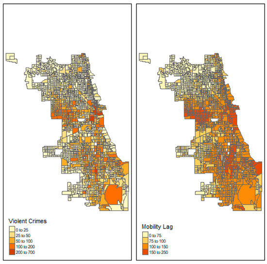
Figure 1.
Chicago Violent Crimes and Mobility Lag.
To operationalize spatial lag, I look at the census block groups that are contiguous with a given census block group. This approach aligns with past research [8]. Subsequently, I specifically operationalize spatial lag as the proportion of contiguous tracts that experienced a violent crime in the previous hour. As an example, if a given neighborhood was contiguous with five other neighborhoods and exactly one of them experienced a violent crime, the spatial lag for the given neighborhood in the next hour would be 0.2. Spatial lag, as I conceptualize it here, effectively refers to the level of violence in spatially proximal neighborhoods in the preceding hour. This measure of spatial lag provides a variable by which to test if spatial pathways predict the diffusion of violent crime.
I estimate a two-way fixed effects model for all three cities in the exact same form. For New York City, 309 census block groups and 28 h of the year were dropped because no violent crimes were reported there or then. For Los Angeles, 73 census block groups and 162 h of the year were dropped because no violent crimes were reported there or then. For Chicago, 21 census block groups and 55 h of the year were dropped because no violent crimes were reported there or then.
Table 1, Table 2 and Table 3 contain summary statistics for New York City, Los Angeles and Chicago, respectively.

Table 1.
Summary statistics for New York City.
Table 2.
Summary statistics for Los Angeles.
Table 3.
Summary statistics for Chicago.
My preferred model specification can be written as follows:
where is an indicator variable denoting whether or not CBG i experienced any violent crimes in hour t. represents the natural log of the number of visitors to CBG i in hour t. represents the natural log of the number of residents of CBG i at home in hour t. represents the sum of In-degree violence and out-degree violence for CBG i in hour t − 1. represents the spatial lag for CBG i in hour t − 1. represents fixed effects for all CBGs. represents fixed effects for all hours in 2019. is an error term with the assumed statistical properties for a two-way fixed effect logit model.
The intuition behind the model is that the incidence of violence may vary substantially between certain neighborhoods and certain periods of time. Conditioning on the neighborhood and time period, I expect time-varying covariates for the number of people in the neighborhood to be a significant predictor of the incidence of violence. I also expect mobility lag to be a significant predictor of violent crime [33]. While I do not necessarily expect spatial lag to be significant, I do expect any significant effect that is to occur to be minute in comparison the effect size for mobility lag. Interpretation-wise, a positive and significant coefficient for mobility lag suggests that mobility pathways can predict the diffusion of violent crime between neighborhoods, while a positive and significant coefficient for spatial lag suggests that pathways related simply to spatial proximity can predict the diffusion of violent crime between neighborhoods. Ultimately, I believe the model I use here is quite parsimonious and aligns with past criminological research by taking advantage of two-way fixed effects and including the most theoretically meaningful time-varying covariates.
5. Results
Table 4 presents the main model results for New York City. Model one estimates the presence of hourly violence based on logged visitors and logged population at home that hour. Visitors are a strong predictor of the likelihood of violence, while population at home makes a more modest contribution. This aligns with recent research, which has found the volume and composition of visitors to an area to predict violence [28,29]. Model two adds in lagged violent crime, a dichotomous variable indicating whether or not a violent crime was reported in the census block group in the previous hour. Interpreting these results as a risk ratio, which is reasonable given the rarity of the outcome, the presence of violent crime in the prior hour increases the risk of a violent crime in the current hour by 116.4%.
Table 4.
New York City Hourly Violent Crime Models.
Model three adds spatial lag, which is operationalized here as the fraction of spatially contiguous neighborhoods that experienced a violent crime in the previous hour. The estimates reveal a positive effect of spatial lag on the odds of a violent crime, significant at p < 0.01. Assuming a neighborhood is bordered by five neighborhoods, and one of them experiences a violent crime in the previous hour, the risk of a violent crime in the subsequent hour would be increased by 9.6% relative to if none of the contiguous neighborhoods had experienced any violent crime.
Model four excludes spatial lag but includes mobility lag. Mobility lag is operationalized here as the sum of all neighborhoods that experienced a violent crime in the previous hour, weighting by the percent of visits made by residents of the target neighborhood to those neighborhoods and by the percent of visitors to the target neighborhood that are from those neighborhoods. The coefficient estimate reveals this is a strong predictor of the risk of violent crime, significant at p < 0.001. For example, if a neighborhood that sends and receives 2.5% of the visitors to another neighborhood experiences a crime in a particular hour, the risk of the other neighborhood experiencing a neighborhood increases by 8.9%.
Model five includes both spatial lag and mobility lag. The effect of spatial lag becomes negative here but is not statistically significant. The effect of mobility lag actually slightly increases. Ultimately, the results indicate that any effect of spatial lag in New York City can be explained by mobility lag. Mobility lag appears to be an essential form of relation through which violence in one hour can predict violence in the next.
Table 5 and Table 6 present the results of models for Los Angeles and Chicago. The results mostly follow those of New York City. Visitors and population at home are important predictors of violent crime, with visitors being a dominant driver. Lagged violent crime is a consistently strong predictor, although slightly less so in Los Angeles and Chicago (73.7% and 55.7% increase in risk) compared to New York City (116.4%).
Table 5.
Los Angeles Hourly Violent Crime Models.
Table 6.
Chicago Hourly Violent Crime Models.
Notably, spatial lag is not a significant predictor of violent crime in Los Angeles or Chicago. Both coefficients are positive, however, suggesting the substantially smaller number of observations in Los Angeles and Chicago (and subsequent reduced statistical power) may be responsible for why spatial lag is not significant in either city. In either case though, mobility lag is a significant predictor. Again, the effect is smaller in Los Angeles or Chicago versus New York City. If a neighborhood that sends and receives 2.5% of the visitors to another neighborhood experiences a violent crime in a particular hour, the risk of the other neighborhood experiencing a violent crime increases by 8.9% in New York City, 3.7% in Los Angeles, and 2.8% in Chicago. In all three cases, when spatial lag and mobility lag are included in a model, the effect of spatial lag is negative and non-significant, while the effect of mobility lag is positive and significant.
6. Discussion
The diffusion of gun violence has been well-studied within criminology. Most recently, a spatiotemporal test found that while gun violence is contagious, diffusion is limited to short distances, 126 m, and short times, 10 min [9]. While this research makes a cogent argument, spatiotemporal tests are useless when theory suggests that violence does not spread randomly across space. Indeed, in this research, I find that spatial pathways are insignificant in predicting the diffusion of violent crime between census block groups, while mobility pathways are significant across all three jurisdictions examined. Notably, these three jurisdictions constitute the three largest cities in the United States and vary substantially in geographic and demographic terms.
A notable shortfall of this work is the inability to draw causal inferences from these empirical analyses. A standard method for causal inference in work like this is to utilize weather conditions as an instrumental variable and analyze diffusion between distant people or places. However, this type of analysis necessitates people or places be distant enough that weather conditions may vary substantially, which tends not to be the case with local neighborhoods. Ultimately, the analysis completed here does not justify causal interpretations of a contagion effect.
However, this research does suggest that if a violence contagion did exist, the form through which diffusion would occur would be mobility patterns rather than spatial contiguity. Indeed, this notion aligns closely with theory. Retaliatory acts constitute a central mechanism through which violence contagion may manifest [9]. Such retaliatory acts should constitute a network of people whose movement patterns are approximately captured by aggregated, nuanced mobility metrics, not simply spatially proximal patterns of movement.
In addition to a contagion effect, mobility patterns may predict violent crime diffusion as a result of shared-exposure bias. Various common exposures tend to cause violence, and mobility ties may indicate that residents of different neighborhoods share these common exposures. Spatially proximal neighborhoods need not be strongly connected through mobility patterns, so the same is not necessarily true for spatially proximal neighborhoods.
If violence is contagious and spreads through mobility patterns, such a finding would have substantial implications for neighborhood inequality in contagion-induced violence. Specifically, a major implication would be that neighborhoods connected through mobility patterns to violent neighborhoods would experience more contagion-induced violence. Notably, recent analyses of violence and other adverse neighborhood outcomes find that mobility connections with disadvantaged neighborhoods is an extremely powerful predictor [28,31]. Furthermore, connections to disadvantaged neighborhoods also tend to be racially unequal. Since disadvantage and violence are highly correlated, contagious violence may ultimately be even more concentrated in already-violent neighborhoods and also may concentrate in Black neighborhoods. Future research needs to better assert the validity of these claims though.
The ability to predict violent crime is valuable regardless of the awareness of the causal mechanism. For example, research using social networks to predict the diffusion of gun violence has blossomed into targeted violence prevention programs in Chicago [34]. This program, and other similar ones, operate outside the criminal justice system and provide alternatives to traditional policing in preventing violence. While this analysis is done over the short term, this work lays a blueprint for utilizing mobility patterns to predict violence before it happens, which may eventually be usable in preventing violence. Future research should build off this work by further disentangling the mechanisms that make mobility patterns meaningful, and policy interventions should consider utilizing these findings in creating violence prevention programs.
7. Conclusions
In this work, I compared mobility and spatial pathways in the hourly patterning of violent crime in New York City, Los Angeles, and Chicago. Across all three cities, I find that recent violence in the neighborhoods a neighborhood is connected to through mobility ties can strongly predict that neighborhood’s odds of violent crime in the subsequent hour. Furthermore, spatial proximity has no significant effect on the likelihood of violent crime after controlling for mobility ties in any of the three cities. I encourage future research on violence contagion to more greatly consider mobility patterns as a potential pathway and empirically take advantage of the rich data that has become recently available.
Supplementary Materials
The following supporting information can be downloaded at: https://www.mdpi.com/article/10.3390/urbansci6040074/s1, Figure S1. Manhattan, Figure S2. Brooklyn, Figure S3. Queens, Figure S4. Bronx, Figure S5. Staten Island, Figure S6. Los Angeles.
Funding
This research received no external funding.
Institutional Review Board Statement
Not applicable.
Informed Consent Statement
Not applicable.
Data Availability Statement
Data sharing is not allowed because of Safegraph’s terms of service.
Conflicts of Interest
The authors declare no conflict of interest.
References
- Buka, S.L.; Stichick, T.L.; Birdthistle, I.; Earls, F.J. Youth exposure to violence: Prevalence, risks, and consequences. Am. J. Orthopsychiatry 2001, 71, 298–310. [Google Scholar] [CrossRef] [PubMed]
- Dodge, K.A.; Bates, J.E.; Pettit, G.S. Mechanisms in the Cycle of Violence. Science 1990, 250, 1678–1683. [Google Scholar] [CrossRef]
- Galster, G.C. The mechanism (s) of neighbourhood effects: Theory, evidence, and policy implications. In Neighbourhood Effects Research: New Perspectives; Springer: Dordrecht, The Netherlands, 2012; pp. 23–56. [Google Scholar]
- Heissel, J.A.; Sharkey, P.T.; Torrats-Espinosa, G.; Grant, K.; Adam, E.K. Violence and Vigilance: The Acute Effects of Community Violent Crime on Sleep and Cortisol. Child Dev. 2017, 89, e323–e331. [Google Scholar] [CrossRef] [PubMed]
- Margolin, G.; Gordis, E.B. Children’s exposure to violence in the family and community. Curr. Dir. Psychol. Sci. 2004, 13, 152–155. [Google Scholar] [CrossRef]
- Sharkey, P.T.; Tirado-Strayer, N.; Papachristos, A.V.; Raver, C.C. The Effect of Local Violence on Children’s Attention and Impulse Control. Am. J. Public Health 2012, 102, 2287–2293. [Google Scholar] [CrossRef]
- Blumstein, A. Youth Violence, Guns, and the Illicit-Drug Industry. J. Crim. Law Criminol. 1995, 86, 10. [Google Scholar] [CrossRef]
- Cohen, J.; Tita, G. Diffusion in homicide: Exploring a general method for detecting spatial diffusion processes. J. Quant. Criminol. 1999, 15, 451–493. [Google Scholar] [CrossRef]
- Loeffler, C.; Flaxman, S. Is Gun Violence Contagious? A Spatiotemporal Test. J. Quant. Criminol. 2017, 34, 999–1017. [Google Scholar] [CrossRef]
- Papachristos, A.V.; Braga, A.A.; Piza, E.; Grossman, L.S. The company you keep? the spillover effects of gang membership on individual gunshot victimization in a co-offending network. Criminology 2015, 53, 624–649. [Google Scholar] [CrossRef]
- Papachristos, A.V.; Wildeman, C.; Roberto, E. Tragic, but not random: The social contagion of nonfatal gunshot injuries. Soc. Sci. Med. 2015, 125, 139–150. [Google Scholar] [CrossRef]
- Tobler, W.R. A Computer Movie Simulating Urban Growth in the Detroit Region. Econ. Geogr. 1970, 46, 234–240. [Google Scholar] [CrossRef]
- Brantingham, P.J.; Yuan, B.; Herz, D. Is Gang Violent Crime More Contagious than Non-Gang Violent Crime? J. Quant. Criminol. 2020, 37, 953–977. [Google Scholar] [CrossRef]
- Tita, G.E.; Greenbaum, R.T. Crime, neighborhoods, and units of analysis: Putting space in its place. In Putting Crime in Its Place; Springer: New York, NY, USA, 2009; pp. 145–170. [Google Scholar]
- Graif, C.; Lungeanu, A.; Yetter, A.M. Neighborhood isolation in Chicago: Violent crime effects on structural isolation and homophily in inter-neighborhood commuting networks. Soc. Netw. 2017, 51, 40–59. [Google Scholar] [CrossRef]
- Sharkey, P.; Marsteller, A. Neighborhood Inequality and Violence in Chicago, 1965–2020. Univ. Chic. Law Rev. 2022, 89, 3. [Google Scholar]
- Lester, D. Temporal variation in suicide and homicide. Am. J. Epidemiol. 1979, 109, 517–520. [Google Scholar] [CrossRef] [PubMed]
- Bridges, F.S. Rates of Homicide and Suicide on Major National Holidays. Psychol. Rep. 2004, 94, 723–724. [Google Scholar] [CrossRef]
- Cheatwood, D. The effects of weather on homicide. J. Quant. Criminol. 1995, 11, 51–70. [Google Scholar] [CrossRef]
- Ejrnæs, A.; Scherg, R.H. Nightlife activity and crime: The impact of COVID-19 related nightlife restrictions on violent crime. J. Crim. Justice 2022, 79, 101884. [Google Scholar] [CrossRef] [PubMed]
- Duke, A.A.; Smith, K.M.Z.; Oberleitner, L.M.S.; Westphal, A.; McKee, S.A. Alcohol, drugs, and violence: A meta-meta-analysis. Psychol. Violence 2018, 8, 238–249. [Google Scholar] [CrossRef]
- Campbell, C.A.; Hahn, R.A.; Elder, R.; Brewer, R.; Chattopadhyay, S.; Fielding, J.; Naimi, T.S.; Toomey, T.; Lawrence, B.; Middleton, J.C.; et al. The Effectiveness of Limiting Alcohol Outlet Density as a Means of Reducing Excessive Alcohol Consumption and Alcohol-Related Harms. Am. J. Prev. Med. 2009, 37, 556–569. [Google Scholar] [CrossRef]
- Copus, R.; Laqueur, H. Entertainment as Crime Prevention: Evidence from Chicago Sports Games. J. Sports Econ. 2018, 20, 344–370. [Google Scholar] [CrossRef]
- Elwert, F.; Christakis, N.A. Wives and ex-wives: A new test for homogamy bias in the widowhood effect. Demography 2008, 45, 851–873. [Google Scholar] [CrossRef] [PubMed]
- Feld, S.L. Why your friends have more friends than you do. Am. J. Sociol. 1991, 91, 1464–1477. [Google Scholar] [CrossRef]
- Christakis, N.A.; Fowler, J.H. Social network sensors for early detection of contagious outbreaks. PLoS ONE 2010, 5, e12948. [Google Scholar] [CrossRef] [PubMed]
- Ben Sliman, M.; Kohli, R. Asymmetric relations and the friendship paradox. Columbia Bus. Sch. Res. Pap. 2018, 18–73. [Google Scholar] [CrossRef]
- Levy, B.L.; Phillips, N.E.; Sampson, R.J. Triple Disadvantage: Neighborhood Networks of Everyday Urban Mobility and Violence in U.S. Cities. Am. Sociol. Rev. 2020, 85, 925–956. [Google Scholar] [CrossRef]
- Al Boni, M.; Gerber, M.S. Predicting crime with routine activity patterns inferred from social media. In Proceedings of the 2016 IEEE International Conference on Systems, Man, and Cybernetics (SMC), Budapest, Hungary, 9–12 October 2016; pp. 001233–001238. [Google Scholar]
- McCormack, P.D.; Pattavina, A.; Tracy, P.E. Assessing the Coverage and Representativeness of the National Incident-Based Reporting System. Crime Delinquency 2017, 63, 493–516. [Google Scholar] [CrossRef]
- Levy, B.L.; Vachuska, K.; Subramanian, S.V.; Sampson, R.J. Neighborhood socioeconomic inequality based on everyday mobility predicts COVID-19 infection in San Francisco, Seattle, and Wisconsin. Sci. Adv. 2022, 8, eabl3825. [Google Scholar] [CrossRef]
- Wang, Q.; Phillips, N.E.; Small, M.L.; Sampson, R.J. Urban mobility and neighborhood isolation in America’s 50 largest cities. Proc. Natl. Acad. Sci. USA 2018, 115, 7735–7740. [Google Scholar] [CrossRef]
- Malleson, N.; Andresen, M.A. The impact of using social media data in crime rate calculations: Shifting hot spots and changing spatial patterns. Cartogr. Geogr. Inf. Sci. 2014, 42, 112–121. [Google Scholar] [CrossRef]
- Papachristos, A.V.; Kirk, D.S. Changing the street dynamic: Evaluating Chicago’s group violence reduction strategy. Criminol. Public Policy 2015, 14, 525–558. [Google Scholar] [CrossRef]
Publisher’s Note: MDPI stays neutral with regard to jurisdictional claims in published maps and institutional affiliations. |
© 2022 by the author. Licensee MDPI, Basel, Switzerland. This article is an open access article distributed under the terms and conditions of the Creative Commons Attribution (CC BY) license (https://creativecommons.org/licenses/by/4.0/).