Assessment of Air Pollution Mitigation Measures on Secondary Pollutants PM₁₀ and Ozone Using Chemical Transport Modelling over Megacity Delhi, India

Abstract

Sporadic efforts have been introduced to control emissions in Delhi, but the air quality has declined further due to the rapid development of different sectors. In this study, the impact of various mitigation scenarios on air quality for PM₁₀, ozone, and its precursors are studied using a chemical transport model, namely WRF-Chem. The Emission Database for Global Atmospheric Research emission inventory was modified and introduced into the WRF-Chem model to assess the impact of selected emission control scenarios on different sectors. The simulations were conducted with reduced emissions for these sectors over the study domain: (a) implementation of Bharat Stage—VI norms in the transport sector, (b) conversion of fuel from coal to natural gas in the energy sector, and (c) fuel shift to LPG in the residential sector. The transport sector noted a decrease of 4.9% in PM₁₀, 44.1% in ozone, and 18.9% in NOx concentrations with emission reduction measures. In the energy sector, a marginal reduction of 3.9% in NOx concentrations was noted, and no change was observed in PM₁₀ and ozone concentrations. In the residential sector, a decrease of 8% in PM-10, 47.7% in ozone, and 49.8% in NOx concentrations were noted. The VOC-to-NOx ratios were also studied, revealing the ozone production over the study domain was mostly VOC-limited. As the inclusion of control measures resulted in varying levels of reduction in pollutant concentrations, it was also studied in the context of improving the air quality index. The WRF-Chem model can be successfully implemented to study the effectiveness of any regulated control measures.

1. Introduction

The cost of the increasing urbanisation of Delhi city has manifested in the rise of ambient levels of particulate matter and gaseous pollutants due to the unending increase in motor vehicle emissions, along with other anthropogenic sources [1]. Sporadically, efforts have been introduced to improve air quality by adopting measures to control emissions in Delhi. However, the impact of these interventions has been negated by the rapid development of different sectors, which has further deteriorated the air quality [2]. Air pollutants emitted from diverse sources have detrimental impacts, which are of serious concern in urban cities in India.

The emission inventories are compiled for different pollutants from different sectors, such as energy sources—transport, power, industries, residential, etc.—and nonenergy sources, such as fugitive emissions from construction, storage, and handling of fuels, road dust, etc. [3]. An emission inventory generally comprises criteria pollutants, such as nitrogen oxides (NOx), sulphur dioxide (SO₂), carbon monoxide (CO), PM₁₀, and PM_2.5, along with ammonia (NH₃) and volatile organic compounds (VOCs), which serve as precursors to secondary particulate matter (PM) and ozone [4]. Besides these pollutants, other greenhouse gases and climate forcers, such as black carbon and brown carbon, are also included in the emission inventories on regional, continental and global scales [5,6,7].

In India, past literature shows efforts to estimate emissions for different sources and pollutants [3,4,8,9,10,11,12,13,14,15,16,17,18,19,20,21]. Most of these studies focussed on the development of emission inventories for Delhi. Gargava et al. [4] derived a speciated PM₁₀ emission inventory for primary species, including elemental carbon, organic carbon, nitrates, sulphates, and metals, for 2007 over the metropolitan area of Delhi. Sahu et al. [22] developed a high-resolution emission inventory of PM_2.5 and PM₁₀ for 2010 over Delhi, which was developed for forecasting air quality during the Commonwealth Games 2010 as part of the System of Air Quality Forecasting and Research (SAFAR) project. Goel and Guttikunda [14] performed a retrospective and prospective analysis of 40 years (1990–2030) of on-road vehicle exhaust emissions and updated dynamic emissions factors for the fleet. Gurjar et al. [16] constructed an emission inventory, employing an emission factor-based approach for source categories over a decade (1990–2000) for Delhi.

The gridded emission inventory is a crucial input to atmospheric models for simulating atmospheric pollutants and an essential component of an air quality management plan that enables assessment of the progress in achieving the cleaner air goal over time [3]. Mohan et al. [17] prepared a gridded emission inventory for Delhi from annual emission data taken over a decade (1990–2000) using a top-down approach. The annual emission inventories compiled over defined regions can be apportioned in time and space to assist air quality modelling, relating emissions to ambient pollutant concentrations [4,23]. Such atmospheric chemical modelling facilitates the appropriate selection of emission reduction measures and evaluation of the adverse effects on human health, climate, visibility, cultural heritage, etc. [4]. An essential component of an air quality management strategy is the effective inclusion of emission reduction scenarios using the atmospheric chemical models. With this background, we aim to assess the improvement in air quality for specific emission reduction scenarios in the megacity Delhi in the National Capital Region (NCR) of India. The study employs a chemical transport model, namely WRF-Chem into which a user-modified global emission inventory, EDGAR, has been incorporated. The study also examines the role of atmospheric chemistry in influencing ambient levels of key secondary pollutants, such as ozone and particulate matter, in Delhi for the different control options, to understand the implications for regulatory purposes.

2. Emission Inventory

EDGAR (Emission Database for Global Atmospheric Research) provides global anthropogenic emissions of greenhouse gases and air pollutants by country and on spatial grid. The EDGAR emission dataset used in the present study is Hemispheric Transport of Air Pollution (HTAP). EDGAR compiled the HTAP inventory, which is based on the Model Intercomparison Study for Asia (MICS-Asia), Environmental Protection Agency (EPA) for USA, EPA and Environment Canada (EPA-US/Canada), and Netherlands Organisation for Applied Scientific Research (TNO) for Europe, at a spatial resolution of 0.1° × 0.1°. The dataset includes emissions for CO, SO₂, NOx, NMVOC, PM₁₀, PM_2.5, NH₃, BC, and OC using regional emission grid maps for the years 2008 and 2010, at annual and monthly temporal resolutions [24]. The dataset consists of emissions from seven sectors of human activities, which are residential, power, industry, ground transport, agriculture, aviation, and shipping, to yield global, sector-specific grid maps for each year and substance. For Asia, all emissions from all sectors are included except international aviation, international shipping, and agricultural waste burning [24]. The EDGAR inventory was selected as it is readily available on the global domain, compared to the site-specific inventory for the regional domain. Although the selected inventory is relatively coarse, it incorporates all major sector contributions to each pollutant, similar to any site-specific inventory.

3. Methodology

3.1. Contribution of Different Emission Sectors

The primary step in air quality control planning is identifying significant sources of pollutants’ emissions. Hence, the contribution of different emissions sectors was quantified to effectively assess mitigation measures. Figure 1 represents the contribution of different sectors to PM₁₀ and NOx emissions based on the EDGAR emission inventory over India’s NCR for June 2010 and December 2010. It was noted that the total PM₁₀ and NOx emissions in December 2010 were higher than those in June 2010, but the relative sectoral contribution was similar in both months. The relative reduction being the same led to a similar conclusion. Further, the secondary reaction rates were higher in the summer season (June). Thus, considering conservative emission estimates, simulations were performed for the entire month of June 2010 for implementation of the emission reduction measures. The simulation period was representative of the entire year, based on the month experiencing high pollution levels due to episodes of dust storms along with sector contribution to the pollutants.

3.2. Selection of Air Pollution Control Scenarios

This section discusses the control scenarios adopted for this study. The emissions were reduced in the EDGAR emission inventory for the Delhi NCR domain to assess the air pollution control scenarios.

As Delhi has multiple sources, such as vehicles, industries, residential, etc., it is critical to examine the constraints, such as technical, fiscal, administrative, and others, for proposing emission scenarios, with a view to understand their applicability to the city. Under the aegis of the Central Pollution Control Board, Government of India, a detailed study was conducted by the National Environmental Engineering Research Institute (NEERI) to assess air pollutant levels in different parts of Delhi [1]. The study listed numerous emission control options for Delhi after projection analysis. The emission reduction scenarios that were adopted in the present study are based on the NEERI report [1]. The three emission control options considered for this study are presented in

Table 1. Proposed emission scenarios for the different sectors for PM and NOx emissions (Source: NEERI, 2008).

Sector	Scenario	PM	NOx
Transport	Implementation of BS-VI	−29.1%	−23.6%
Energy	Coal to NG	−0.06%	−36.69%
Residential	Fuel shift to LPG	−68.4%	−69.47%

. These three different mitigation scenarios were accomplished with a reduction in the (a) transport sector, with the implementation of Bharat Stage VI (BS-VI) norms, which are emission standards placed by the government to regulate the output of air pollutants from internal combustion engines and spark-ignition engine equipment including motor vehicles [25], similar to Euro-6 standards in the European Union; (b) energy sector, by converting coal-based power plants and industries to natural gas; and (c) residential sector, with a fuel shift to liquefied petroleum gas (LPG). Improvement in the air quality was assessed based on reduction in PM and NOx emissions for each of the three control scenarios. The control scenario for the transport sector involved the implementation of Bharat Stage VI (BS-VI) emission norms for the new vehicles, with an expected reduction of 29.1% in PM emissions and 23.6% in NOx emissions. For the energy sector, the conversion of coal-based power plants and industries to natural gas (NG) led to a reduction in PM emissions of 0.06% and in NOx emissions of 36.69%. In power plants and industries, natural gas is considered a cleaner and better fuel option than coal [1]. In the residential sector, the control measure introduced a shift to LPG, resulting in a 68.4% reduction in PM emissions and a 69.47% reduction in NOx emissions. LPG is considered a cleaner fuel, compared to kerosene, wood, and coal, for domestic cooking as well as commercial units such as restaurants, hotels, and bakeries [1].

3.3. Incorporation of Mitigation Scenarios in WRF-Chem

The WRF-Chem model version 3.5 was employed to assess the changes in simulated pollutant concentrations after adopting the aforementioned mitigation measures. The physical parameterisation and chemistry schemes were selected based on the various sensitivity analysis studies performed for the same region [26,27,28]. These were the Lin et al. [29] microphysics parameterisation; the Noah land surface model [30]; the ACM2 PBL scheme [31]; the Kain–Fritsch cumulus parameterisation scheme [32]; the Goddard scheme for atmospheric shortwave radiation; the rapid radiative transfer model (RRTM) for longwave radiation; the MOSAIC aerosol scheme, coupled with the CBMZ gas-phase mechanism [33]; and the Madronich [34] photolysis scheme.

The WRF-Chem model requires terrestrial and meteorological data inputs. USGS 24 classification category land-use data was used to interpolate topography and land use with a spatial resolution of 30″. Meteorological initial and boundary conditions were obtained from the National Centre for Environmental Prediction (NCEP), with final analysis data (FNL) of 1° resolution. These datasets can be downloaded from the WRF model website [35]. As described in the previous section, the model’s chemical module requires emission input obtained from EDGAR. Chemical initial and boundary conditions were extracted from the model for ozone and related chemical tracers, version 4 (MOZART-4) global chemical transport model. The simulation domain is shown in Figure 2. The parent domain covers part of Asia at a resolution of 54 km × 54 km, the first nested domain surrounds India at 18 km × 18 km, the second nested domain at a resolution of 6 km x 6 km and the third nested domain encapsulates the National Capital Region (NCR). The fourth domain encompassing the NCR includes the National Capital Territory (NCT) of Delhi and surrounding areas (i.e., 22 districts) of Haryana (13 districts), Uttar Pradesh (7 districts), and Rajasthan (2 districts), representing the land-use land-cover of the region, as designated by the U.S. Geological Survey (USGS) 24 category dataset. The dominant land-use land-cover across the entire region is dry cropland, with some parts of Delhi under the urban and built-up land category. The changes in emissions were implemented for the Delhi region in the third nested domain.

The emission control scenarios adopted from NEERI [1] were implemented by modifying the monthly EDGAR-HTAP emission inventory for PM₁₀ and NOx emissions for each of the three scenarios mentioned in Table 1. The emissions were modified using the HDFView version 3 tool. HDFView is a Java-based tool that allows browsing and editing of HDF4- and HDF5-format files. The editing features of the tool allow the user to modify, create, and delete the value of the HDF objects and attributes. HDFView enables the user to view the data content as an image, plain text, or a table [36]. The original and modified EDGAR-HTAP emissions for NOx and PM₁₀ for the three control scenarios over Delhi are shown as a grid in Tables S1 to S6 in the supplementary material.

The original and modified emissions were introduced in the WRF-Chem model, and the impact of the reduction in emissions was studied using the simulated pollutant concentrations. Daily average values of PM₁₀ and NOx and 8-h average values of ozone were analysed to study the impact of the sector-wise implementation of emission reduction. These averaging intervals for PM₁₀, NOx_, and ozone were selected based on the air quality standards in India [37]. These ambient concentrations were averaged for the air quality monitoring stations in Delhi.

4. Results & Discussion

This section evaluates the impact of the selected emission reduction scenarios on ambient concentrations over Delhi using the WRF-Chem model. The EDGAR emission inventory was edited to indicate the reductions, and then the modelling system was used to investigate the differences between the various control scenarios and the nonreduction simulation. The following subsections discuss the same for pollutants PM₁₀ and ozone. In a previous study [26], the authors discussed the model validation of these two pollutants using the WRF-Chem model and EDGAR emission inventory for the same period and domain. It was noted that the fractional bias for PM₁₀ and ozone was 0.01 and −0.55, respectively. The value of the index of agreement was 0.71 for PM₁₀ and 0.56 for ozone [26]. The mentioned validation provided the confidence to perform the assessment study discussed in the following section.

4.1. PM₁₀

Primary particulate matter is directly emitted to the atmosphere, which can be controlled at the emission source. The NOx emissions are partly transformed into particles by photochemical reactions in the atmosphere, thereby forming secondary particulate matter. The nitrogen dioxide (NO₂) is oxidised to nitric acid (HNO₃), which in turn reacts with ammonia (NH₃) to form ammonium nitrate (NH₄NO₃) particles [38].

NH_{3 (g)} + HNO_{3 (g)} → NH₄NO_{3 (s,aq)}

(1)

Therefore, reductions in both PM₁₀ and NOx are studied to understand the impact on pollutant concentrations. Figure 3 shows the reduction observed for simulated PM₁₀ concentrations for the three emission control scenarios. In the residential sector, with a decrease of 68.4% in PM₁₀ emissions, the simulated PM₁₀ concentrations showed a decrease that varied from 5.5 µg m⁻³ to 38 µg m⁻³. A decrease of approximately 29.1% in PM₁₀ emissions in the transport sector resulted in a decrease of 1.5–31 µg m⁻³ in PM₁₀ concentrations. For a 68.4% reduction in PM₁₀ emissions in the residential sector, an average 8% decrease was observed in PM₁₀ concentration. In the transport sector, a decrease of approximately 5% was noted in PM₁₀ concentration as a 29.1% reduction in PM₁₀ emissions. It was noted that, for the energy sector, because the change in emissions for PM₁₀ was negligible, no change was observed for the simulated PM₁₀ concentrations.

Figure 4 shows the reduction observed for simulated NO_X concentrations for the three emission control scenarios. A slight decrease of 0.1 µg m⁻³ to 2 µg m⁻³ was observed with energy emission reduction scenario for NOx simulated concentrations with a 36.69% decrease in NOx emissions. A decrease of 69.47% in NOx emissions in the residential sector led to a significant decrease, ranging between 30 µg m⁻³ and 56 µg m⁻³, in simulated NO_X concentrations. Similarly, a decrease of approximately 23.6% in NO_X emissions in the transport sector resulted in a reduction of 5–26 µg m⁻³ in NO_X concentrations. A reduction of 69.47% in NOx emissions in the residential sector led to an average decrease of 49.8% in NOx concentration. In the transport sector, a decrease of approximately 18.9% is noted in NOx concentration with a 23.6% reduction in NOx emissions. NOx concentrations decreased by approximately 3.9% with a 36.69% reduction in NOx emissions in the energy sector.

4.2. Ozone

As ozone is a secondary pollutant formed by photochemical reactions of NOx and VOCs, the reduction in simulated ozone concentrations is studied with respect to reduction in NOx emissions. The important chemical reactions resulting in ozone formation are shown below [27].

HO₂ + NO → OH +NO₂

(2)

CH₃O₂ + NO → CH₃O + NO₂

(3)

$${\mathrm{NO}}_2+\mathrm{h}\mathsf{\nu }\stackrel{{\mathrm{O}}_2}{\to }\mathrm{NO}+{\mathrm{O}}_3$$

(4)

Figure 5 shows the reduction observed for simulated ozone concentrations for the three emission control scenarios. For the residential sector, with a decrease of 69.47% in NOx emissions, the simulated ozone concentrations showed a decrease ranging between 4 µg m⁻³ and 38.5 µg m⁻³. With a decrease of approximately 23.6% in NOx emissions in the transport sector, the decrease noted for ozone concentrations was between 3 µg m⁻³ and 37 µg m⁻³. For a 69.47% reduction in NOx emissions in the residential sector, a decrease of approximately 47.7% was observed in ozone concentration. In the transport sector, a decrease of about 44.1% was noted in ozone concentration with a 23.6% reduction in NOx emissions. While a slight reduction in NOx concentrations was observed for the NOx emission reduction in the energy sector, no change was noticed in ozone concentrations. Thus, change in the energy sector did not contribute to ozone production, unlike the other sectors, such as transport and residential.

The above-discussed sector-wise percentage reduction in emissions and the corresponding reduction in ambient concentrations are consolidated in

Table 2. Sector-wise percentage reduction in emissions and the corresponding reduction in ambient concentrations.

Sector	Emission Reduction (%)		Original Concentration (µg m−3)			Concentration Reduction (µg m−3)
	PM10	NOx	PM10	NOx	Ozone	PM10	NOx	Ozone
Transport	−29.1%	−23.6%	52–445	62–104	6–73	1.5 to 31 (5%)	5 to 26 (18.9%)	3 to 37 (44.1%)
Energy	−0.06%	−36.69%	52–445	62–104	6–73	-	0.1 to 2 (3.9%)	-
Residential	−68.4%	−69.47%	52–445	62–104	6–73	5.5 to 38 (8%)	30 to 56 (49.8%)	4 to 38.5 (47.7%)

.

Ozone is produced by a cycle of reactions involving two basic pollutants: NOx and VOCs. Thus, it is vital to understand the role of both VOCs and NOx emissions in ozone formation. For this purpose, VOCs-to-NOx ratios were studied. Figure 6 represents scatter plots of NMVOCs to NOx ratio. An area is considered VOC-limited at low VOCs-to-NOx ratio, i.e., less than approximately 4 to 1. For a high ratio, greater than approximately 15 to 1, the region is classified as NOx-limited. In a NOx-limited regime, O₃ concentrations increase with increasing NOx and are insensitive to hydrocarbons, while in a VOC-limited regime, O₃ concentrations increase with increasing hydrocarbons (VOCs). Therefore, the formulation of a successful strategy against O₃ pollution requires knowledge of the chemical regime for O₃ production. In a VOC-limited regime, VOC emission controls cause a decrease in O₃ levels. However, in the NOx-limited regime, VOC emission controls are of no benefit in decreasing O₃ [39]. Scatter plots of NMVOCs to NOx ratio show whether the ozone concentration production is VOCs limited or NOx limited. In Figure 6, it can be inferred that for all simulations performed, ozone production was NMVOC limited. Various sources contribute to VOCs emissions, such as vehicular exhaust, refuelling stations, industrial hubs, diesel generator sets, etc. Srivastava et al. [40] reported source contribution to total VOCs for a traffic junction in Delhi as 43% from diesel exhaust, 24% from gasoline, 19% from evaporative, and 14% from other sources. Overall, in Delhi, approximately 26% to 54% of VOCs are emissions from diesel internal combustion engines [40]. As ozone production is VOC-limited, reducing VOC emissions can further help reduce ozone concentrations.

4.3. Air Quality Index Assessment

The wind speed and direction simulated by the model were validated along with the assessment of the air quality of Delhi for PM₁₀ and ozone. Wind roses for both observed and simulated data (averaged over the simulation period) are plotted in Figure 7. In the present study, the meteorology was kept uniform in all simulation cases in order to effectively understand the changes in concentration from emissions only. Hence, the validation of the wind was undertaken for the simulated wind from the case with no control measures. Figure 7a shows the observed winds flowing dominantly from the west, ranging from 3.6 to 8.8 ms⁻¹. While the simulated winds (Figure 7b) showed a similar directional pattern, the model slightly overestimated wind speed. Although the focus of this study was on assessing the changes in modelled pollutant concentrations due to changes in emission inputs, the validation of wind was performed to examine the model performance for meteorological variables. It was noted that the wind was well simulated by the WRF-Chem model for the study period. Extensive temperature and wind speed validation is not included in this manuscript. A previous study by Mohan and Gupta [26] examined and inferred that the model performs extremely well for both parameters with low RMSEs of approximately 2.45 °C for temperature and 2.08 ms⁻¹ for wind speed, with slight overestimation. It is assumed that model performance based on the uniform meteorological conditions in all emission scenarios will influence the concentrations to a similar extent for all practical purposes.

Further, air quality was assessed with and without control scenarios, based on Air Quality Index (AQI). The AQI assessment is an effective tool for validating model performance, as it helps quantify air quality in terms of adverse health effects on humans. The AQI is a system for transforming air pollution levels into a single number that aims to provide information about air quality in simple terms to the general public [41]. The AQI varies from 0 to 500; the higher the AQI value, the greater the level of air pollution and the greater the health concern given in Table 3. The general equation for subindex (I_i) for a given pollutant concentration C_p, is calculated as follows:

$$I_i=[\{(I_{HI}-I_{LO})/(B_{HI}-B_{LO})\}\ast (C_p-B_{LO})]+I_{LO}$$

where

B_HI = Breakpoint concentration greater than or equal to given concentration

B_LO = Breakpoint concentration less than or equal to given concentration

I_HI = AQI value corresponding to B_HI

I_LO = AQI value corresponding to B_LO

Table 3. Concentration ranges corresponding to AQI categories and their associated health effects for PM₁₀ and ozone (Source: CPCB [41]).

AQI	PM10 (24-h)	O3 (8-h)	Associated Health Effects
Good (0–50)	0–50	0–50	Minimal Impact
Satisfactory (51–100)	51–100	51–100	May cause minor breathing discomfort to sensitive people
Moderately Polluted (101–200)	101–250	101–168	May cause breathing discomfort to people with lung disease such as asthma and discomfort to people with heart disease, children, and older adults
Poor (201–300)	251–350	169–208	May cause breathing discomfort to people with prolonged exposure and discomfort to people with heart disease
Very Poor (301–400)	351–430	209–748	May cause respiratory illness to people with prolonged exposure. Effects may be more pronounced in people with lung and heart diseases
Severe (401–500)	430+	748+	May cause respiratory effects even in healthy people and serious health effects in people with lung and heart diseases. The health effects may be experienced even during light physical activity

Table 3. Concentration ranges corresponding to AQI categories and their associated health effects for PM₁₀ and ozone (Source: CPCB [41]).

AQI	PM10 (24-h)	O3 (8-h)	Associated Health Effects
Good (0–50)	0–50	0–50	Minimal Impact
Satisfactory (51–100)	51–100	51–100	May cause minor breathing discomfort to sensitive people
Moderately Polluted (101–200)	101–250	101–168	May cause breathing discomfort to people with lung disease such as asthma and discomfort to people with heart disease, children, and older adults
Poor (201–300)	251–350	169–208	May cause breathing discomfort to people with prolonged exposure and discomfort to people with heart disease
Very Poor (301–400)	351–430	209–748	May cause respiratory illness to people with prolonged exposure. Effects may be more pronounced in people with lung and heart diseases
Severe (401–500)	430+	748+	May cause respiratory effects even in healthy people and serious health effects in people with lung and heart diseases. The health effects may be experienced even during light physical activity

Figure 8 and Figure 9 display the AQI over Delhi for PM₁₀ and ozone, respectively. For PM₁₀ with original emissions, air quality was 30% ‘satisfactory’, 10% ‘poor’, 45% ‘very poor’ and 15% ‘severe’. With a reduction in transport and residential sector emissions, the days with ‘severe’ air quality were upgraded to ‘very poor’ air quality and 15% of days with ‘good’ air quality was also observed. For ozone with original emissions, the quality of air was 60% ‘good’ and 40% ‘satisfactory’. After implementing transport and residential sector emission reduction, the air quality for ozone further improved to 90% of days with ‘good’ air quality. As discussed above, reducing energy sector emissions did not result in any change in air quality for either of the pollutants. However, with the inclusion of control measures, pollutant concentration levels reduced, resulting in an improvement in air quality. Further, the emission reduction scenarios showed a lesser reduction in PM₁₀ in comparison to ozone. One of the reasons for this may be that PM₁₀ levels are affected by local emissions as well as long-range transport. In con-trast, ozone photochemistry is influenced mainly by local emissions. In this case, the reduction was applied only to NCR emissions. Consequently, there was less reduction in PM₁₀ concentration compared to ozone. A mix of sources contributes to the produc-tion of ambient pollutant concentration in Delhi. The assessment of proposed control measures aids in better understanding the effectiveness of the proposed air quality management plan.

5. Conclusions and Future Work

The present study assesses the impact of emission control options for transport, residential, and energy sectors on improving air quality in Delhi in the National Capital Region of India. The WRF-Chem model and modified EDGAR-HTAP emissions have been used to estimate the reduction in PM₁₀, ozone, and NOx pollution in the city for emission reduction strategies in the three sectors. The main conclusions of the study are as follows:

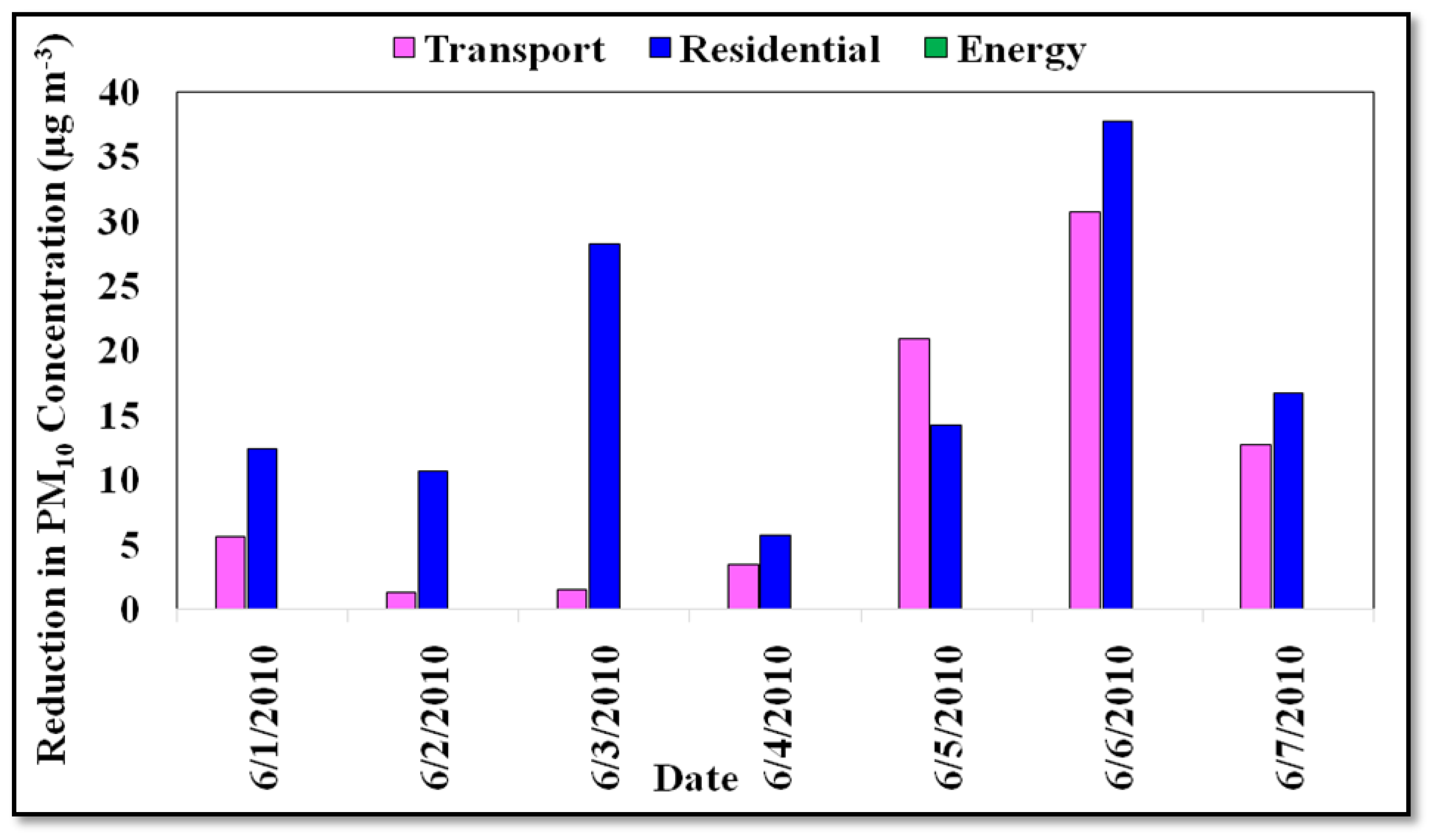
• A decrease of about 8% (5.5 to 38 µg m⁻³) was noted in PM₁₀ concentrations for a complete shift to LPG as fuel in the residential sector. A lesser reduction of about 4.9% (1.5 to 31 µg m⁻³) was achieved in PM₁₀ concentrations by adopting BS-VI emission standards in the transport sector.
• A reduction in residential and transport emissions led to a significant decrease of 47.7% (4 to 38.5 µg m⁻³) and 44.1% (3 to 37 µg m⁻³), respectively, in ozone concentrations.
• A significant decrease of about 49.8% (30 to 56 µg m⁻³) was noted in NOx concentrations in the residential sector, in addition to an 18.9% (5 to 26 µg m⁻³) decrease in the transport sector.
• The strategy of shifting from coal to natural gas in the energy sector showed a marginal decrease of 3.9% (0.1 to 2 µg m⁻³) in NOx concentrations, but negligible change in PM₁₀ and ozone levels.
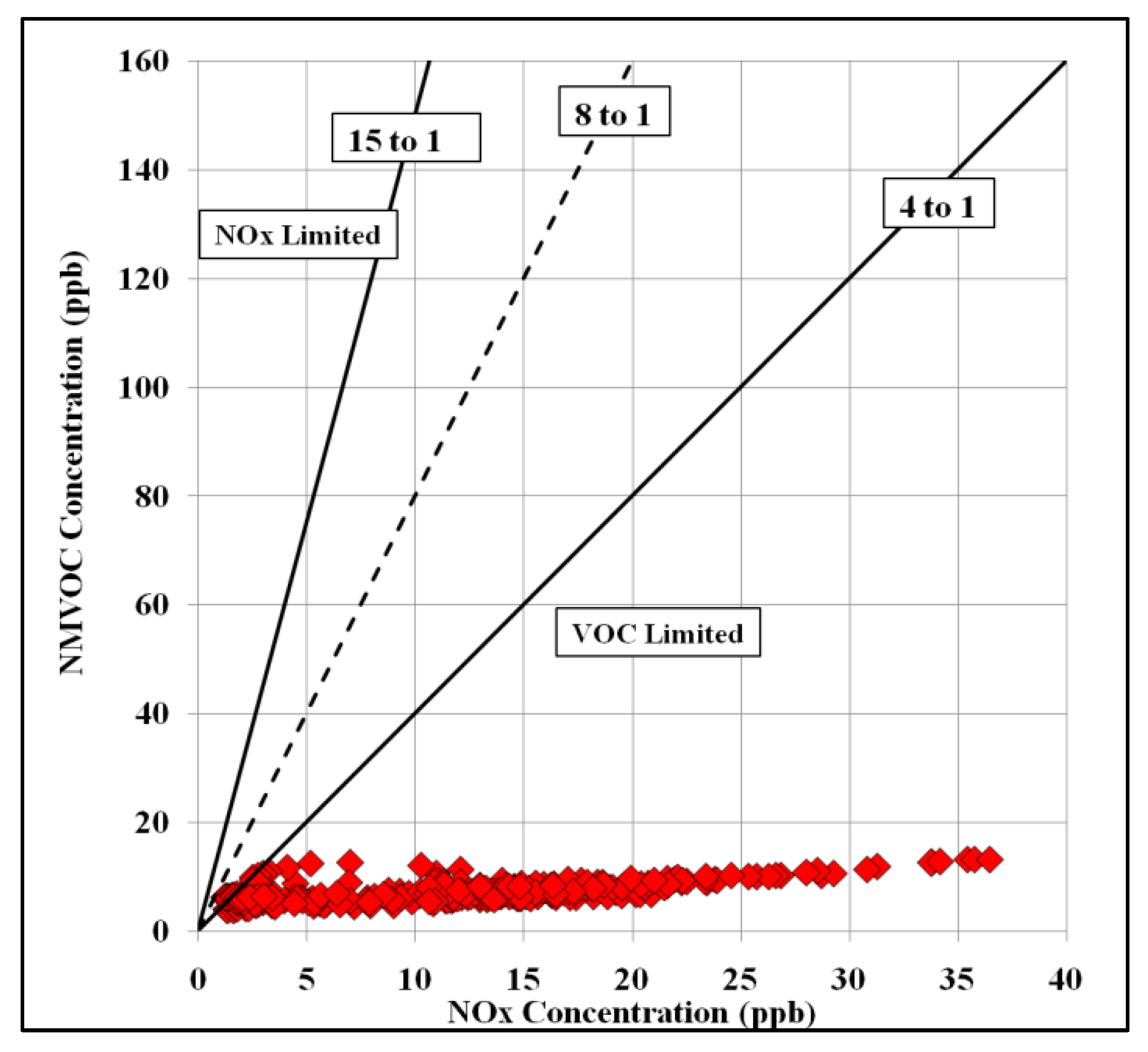
• Ozone production in Delhi was found to be VOC-limited, indicating the importance of reducing VOC emissions for controlling ozone levels in the city.
• Evaluation of the air quality index revealed that ‘good’ AQI, which was initially non-existent, was observed with a 15% frequency with the implementation of emission reduction scenarios. Days reporting ‘severe’ AQI shifted to ‘very poor’ AQI. Similarly, for ozone, the air quality improved, with 90% of days with ‘good’ air quality after implementing control scenarios.
• Lesser reduction in PM₁₀ concentrations compared to ozone is attributed to the difference in the role of long-range transport and local emissions in influencing the ambient levels of these pollutants.

The present study incorporates monthly anthropogenic emission input at 0.1° spatial resolution. As analysed in the study, the contribution of both local and remote sources to pollutant concentrations over Delhi are significant. Thereby, a finer temporal and spatial resolution emission inventory would better capture the region’s daily highs and lows of pollutant concentration. The model could be improved further by incorporating revised rate constants for the given chemical reactions in the mechanism adopted in the model. An updated and more accurate representation of the land-use land-cover (LULC) dataset of the study region as input to the model can also improve simulated PBL height, ventilation coefficient, and ozone and PM₁₀ simulations, which can be further studied in the future.

As Delhi experiences a mix of sources that contribute to the production of ambient pollutant concentration and formation of secondary pollutants, the assessment of proposed control measures via atmospheric chemical modelling could aid in a better understanding of the effectiveness of the proposed air quality management plan. As a part of the National Clean Air Programme (NCAP), India is moving towards the target to reduce PM₁₀ and PM_2.5 pollution in 102 nonattainment cities by 20–30% compared to 2019 levels. Further, in COP26, India committed to Net-Zero Emissions by 2070. Analysis of different control options on air quality is crucial for practical and feasible implementation. This study builds confidence in applying the WRF-Chem model for analysing the impact of future control options in the study area.

References

1. NEERI. Air Quality Assessment, Emission Inventory & Source Apportionment Study for Delhi. APC/NEERI, Nagpur. 2008. Available online: http://cpcb.nic.in/cpcbold/Delhi.pdf (accessed on 10 January 2018).
2. Gulia, S.; Goyal, P.; Prakash, M.; Goyal, S.K.; Kumar, R. Policy Interventions and Their Impact on Air Quality in Delhi City—an Analysis of 17 Years of Data. Water Air Soil Pollut. 2021, 232, 465. [Google Scholar] [CrossRef]
3. Sharma, S.; Kumar, A. (Eds.) Air Pollutant Emissions Scenario for India; The Energy and Resources Institute: New Delhi, India, 2016; Available online: https://www.researchgate.net/profile/Sumit_Sharma31/publication/317105835_Air_pollutant_emissions_scenario_for_India/links/5926ac05a6fdcc444348013f/Air-pollutant-emissions-scenario-for-India.pdf (accessed on 10 January 2018).
4. Gargava, P.; Chow, J.C.; Watson, J.; Lowenthal, D.H. Speciated PM10 Emission Inventory for Delhi, India. Aerosol Air Qual. Res. 2014, 14, 1515–1526. [Google Scholar] [CrossRef]
5. Huy, L.N.; Winijkul, E.; Oanh, N.T.K. Assessment of emissions from residential combustion in Southeast Asia and implications for climate forcing potential. Sci. Total Environ. 2021, 785, 147311. [Google Scholar] [CrossRef]
6. Xu, H.; Ren, Y.; Zhang, W.; Meng, W.; Yun, X.; Yu, X.; Li, J.; Zhang, Y.; Shen, G.; Ma, J.; et al. Correction to “Updated Global Black Carbon Emissions from 1960 to 2017: Improvements, Trends, and Drivers”. Environ. Sci. Technol. 2021, 55, 16785. [Google Scholar] [CrossRef]
7. Yan, J.; Wang, X.; Gong, P.; Wang, C.; Cong, Z. Review of brown carbon aerosols: Recent progress and perspectives. Sci. Total Environ. 2018, 634, 1475–1485. [Google Scholar] [CrossRef]
8. Singh, N.; Mishra, T.; Banerjee, R. Emission inventory for road transport in India in 2020: Framework and post facto policy impact assessment. Environ. Sci. Pollut. Res. 2021, 29, 20844–20863. [Google Scholar] [CrossRef]
9. Banerjee, S.; Khan, M.A.; Husnain, M.I.U. Searching appropriate system boundary for accounting India’s emission inventory for the responsibility to reduce carbon emissions. J. Environ. Manag. 2021, 295, 112907. [Google Scholar] [CrossRef]
10. Stewart, G.J.; Nelson, B.S.; Acton, W.J.F.; Vaughan, A.R.; Hopkins, J.R.; Yunus, S.S.; Hewitt, C.N.; Wild, O.; Nemitz, E.; Gadi, R.; et al. Emission estimates and inventories of non-methane volatile organic compounds from anthropogenic burning sources in India. Atmos. Environ. X 2021, 11, 100115. [Google Scholar] [CrossRef]
11. Hakkim, H.; Kumar, A.; Annadate, S.; Sinha, B.; Sinha, V. RTEII: A New High-Resolution (0.1° × 0.1°) Road Transport Emission Inventory for India of 74 Speciated NMVOCs, CO, NOx, NH3, CH4, CO2, PM2.5 Reveals Massive Overestimation of NOx and CO and Missing Nitromethane Emissions by Existing Inventories. Atmos. Environ. X 2021, 11, 100118. [Google Scholar] [CrossRef]
12. Sahu, S.K.; Mangaraj, P.; Beig, G.; Samal, A.; Pradhan, C.; Dash, S.; Tyagi, B. Quantifying the high resolution seasonal emission of air pollutants from crop residue burning in India. Environ. Pollut. 2021, 286, 117165. [Google Scholar] [CrossRef]
13. Raparthi, N.; Phuleria, H.C. Real-world vehicular emissions in the Indian megacity: Carbonaceous, metal and morphological characterization, and the emission factors. Urban Clim. 2021, 39, 100955. [Google Scholar] [CrossRef]
14. Goel, R.; Guttikunda, S.K. Evolution of on-road vehicle exhaust emissions in Delhi. Atmos. Environ. 2015, 105, 78–90. [Google Scholar] [CrossRef]
15. Guttikunda, S.; Calori, G. A GIS based emissions inventory at 1 km × 1 km spatial resolution for air pollution analysis in Delhi, India. Atmos. Environ. 2013, 67, 101–111. [Google Scholar] [CrossRef]
16. Gurjar, B.R.; van Aardenne, J.A.; Lelieveld, J.; Mohan, M. Emission Estimates and Trends (1990–2000) for Megacity Delhi and Implications. Atmos. Environ. 2004, 38, 5663–5681. [Google Scholar] [CrossRef]
17. Mohan, M.; Dagar, L.; Gurjar, B.R. Preparation and Validation of Gridded Emission Inventory of Criteria Air Pollutants and Identification of Emission Hotspots for Megacity Delhi. Environ. Monit. Assess. 2007, 130, 323–339. [Google Scholar] [CrossRef]
18. Mohan, M.; Bhati, S.; Gunwani, P. Emission Inventory of Air Pollutants and Trend Analysis Based on Various Regulatory Measures over Megacity Delhi. In Air Quality: New Perspective; Lopez, G., Ed.; IntechOpen: London, UK, 2012; ISBN 978-953-51-0674-6. [Google Scholar]
19. Nagpure, A.S.; Sharma, K.; Gurjar, B.R. Traffic Induced Emission Estimates and Trends (2000–2005) in Megacity Delhi. Urban Clim. 2013, 4, 61–73. [Google Scholar] [CrossRef]
20. Gurjar, B.R.; Butler, T.M.; Lawrence, M.G.; Lelieveld, J. Evaluation of Emissions and Air Quality in Megacities. Atmos. Environ. 2008, 42, 1593–1606. [Google Scholar] [CrossRef]
21. Behera, S.N.; Sharma, M.; Dikshit, O.; Shukla, S.P. GIS-Based Emission Inventory, Dispersion Modeling, and Assessment for Source Contributions of Particulate Matter in an Urban Environment. Water Air Soil Pollut. 2011, 218, 423–436. [Google Scholar] [CrossRef]
22. Sahu, S.K.; Beig, G.; Parkhi, N.S. Emissions Inventory of Anthropogenic PM2.5 and PM10 in Delhi during Commonwealth Games 2010. Atmos. Environ. 2011, 45, 6180–6190. [Google Scholar] [CrossRef]
23. Hogrefe, C.; Sistla, G.; Zalewsky, E.; Hao, W.; Ku, J.-Y. An Assessment of the Emissions Inventory Processing Systems EMS-2001 and SMOKE in Grid-Based Air Quality Models. J. Air Waste Manage. Assoc. 2003, 53, 1121–1129. [Google Scholar] [CrossRef] [Green Version]
24. Janssens-Maenhout, G.; Crippa, M.; Guizzardi, D.; Dentener, F.; Muntean, M.; Pouliot, G.; Keating, T.; Zhang, Q.; Kurokawa, J.; Wankmüller, R.; et al. HTAP_v2.2: A Mosaic of Regional and Global Emission Grid Maps for 2008 and 2010 to Study Hemispheric Transport of Air Pollution. Atmos. Chem. Phys. 2015, 15, 11411–11432. [Google Scholar] [CrossRef] [Green Version]
25. Borkhade, R.; Bhat, K.S.; Mahesha, G.T. Implementation of Sustainable Reforms in the Indian Automotive Industry: From Vehicle Emissions Perspective. Cogent Eng. 2022, 9, 2014024. [Google Scholar] [CrossRef]
26. Mohan, M.; Gupta, M. Sensitivity of PBL Parameterizations on PM10 and Ozone Simulation Using Chemical Transport Model WRF-Chem over a Sub-Tropical Urban Airshed in India. Atmos. Environ. 2018, 185, 53–63. [Google Scholar] [CrossRef]
27. Gupta, M.; Mohan, M. Validation of WRF/Chem Model and Sensitivity of Chemical Mechanisms to Ozone Simulation over Megacity Delhi. Atmos. Environ. 2015, 122, 220–229. [Google Scholar] [CrossRef]
28. Mohan, M.; Bhati, S. Analysis of WRF Model Performance over Subtropical Region of Delhi, India. Adv. Meteorol. 2011, 2011, 621235. [Google Scholar] [CrossRef] [Green Version]
29. Lin, Y.-L.; Farley, R.D.; Orville, H.D. Bulk Parameterization of the Snow Field in a Cloud Model. J. Appl. Meteorol. Climatol. 1983, 22, 1065–1092. [Google Scholar] [CrossRef] [Green Version]
30. Chen, F.; Dudhia, J. Coupling an Advanced Land Surface–Hydrology Model with the Penn State–NCAR MM5 Modeling System. Part I: Model Implementation and Sensitivity. Mon. Weather Rev. 2001, 129, 569–585. [Google Scholar] [CrossRef] [Green Version]
31. Hong, S.-Y.; Lim, J.-O.J. The WRF Single-Moment 6-Class Microphysics Scheme (WSM6). Asia-Pac. J. Atmos. Sci. 2006, 42, 129–151. [Google Scholar]
32. Kain, J.S. The Kain–Fritsch Convective Parameterization: An Update. J. Appl. Meteorol. 2004, 43, 170–181. [Google Scholar] [CrossRef] [Green Version]
33. Zaveri, R.A.; Peters, L.K. A New Lumped Structure Photochemical Mechanism for Large-Scale Applications. J. Geophys. Res. Atmos. 1999, 104, 30387–30415. [Google Scholar] [CrossRef]
34. Madronich, S. Photodissociation in the Atmosphere: 1. Actinic Flux and the Effects of Ground Reflections and Clouds. J. Geophys. Res. Atmos. 1987, 92, 9740–9752. [Google Scholar] [CrossRef]
35. WRF. 2012. Available online: http://www.mmm.ucar.edu/wrf/users/downloads.html (accessed on 23 March 2012).
36. HDFView. 2018. Available online: https://support.hdfgroup.org/products/java/hdfview/ (accessed on 10 January 2018).
37. CPCB. Annual Report 2013-14; Central Pollution Control Board, Ministry of Environment, Forest & Climate Change: New Delhi, India, 2014. [Google Scholar]
38. Seinfeld, J.H.; Pandis, S.N. Atmospheric Chemistry and Physics: From Air Pollution to Climate Change; John Wiley & Sons: Hoboken, NJ, USA, 2016. [Google Scholar]
39. Jacob, D.J. Introduction to Atmospheric Chemistry; Princeton University Press: Princeton, NJ, USA, 1999. [Google Scholar]
40. Srivastava, A.; Sengupta, B.; Dutta, S.A. Source Apportionment of Ambient VOCs in Delhi City. Sci. Total Environ. 2005, 343, 207–220. [Google Scholar] [CrossRef] [PubMed]
41. CPCB. National Air Quality Index. Control of Urban Pollution Series: CUPS/82/2014-15. 2014. Available online: http://www.indiaenvironmentportal.org.in/files/file/Air%20Quality%20Index.pdf (accessed on 10 January 2018).
Figure 1. Contribution of different sectors to PM10 (a,c) and NOx (b,d) EDGAR emissions over NCR in June 2010 (upper panel) and December 2010 (lower panel) at 0.1° × 0.1° resolution (EDGAR emission inventory).
Urbansci 06 00027 g001
Figure 2. Simulation domains covering Asia (54 km × 54 km resolution) as domain 1, India (18 km × 18 km resolution) as domain 2, parts of north India (6 km × 6 km resolution) as domain 3, and domain 4 enveloping the National Capital Region of India (2 km × 2 km resolution).
Urbansci 06 00027 g002
Figure 3. Reduction plots of simulated PM10 concentrations (µg m−3) representing the difference between original and proposed emission scenarios for transport (pink), residential (blue), and energy (green) sectors, averaged for the entire simulation period over the Delhi domain. Note: No change in concentration was noted in the energy sector.
Urbansci 06 00027 g003
Figure 4. Reduction plots of simulated NOx concentrations (µg m−3) representing the difference between original and proposed emission scenarios for transport (pink), residential (blue), and energy (green) sectors, averaged for the entire simulation period over the Delhi domain.
Urbansci 06 00027 g004
Figure 5. Reduction plots of simulated ozone concentrations (µg m−3) representing the difference between original and proposed emission scenarios for transport (pink), residential (blue), and energy (green) sectors, averaged for the entire simulation period over the Delhi domain. Note: No change in concentration was noted in the energy sector.
Urbansci 06 00027 g005
Figure 6. Scatter plots of NMVOC to NOx ratio over Delhi.
Urbansci 06 00027 g006
Figure 7. Wind rose plots displaying the wind direction and wind speed for simulated period over Delhi. (a) Observed, (b) simulated.
Urbansci 06 00027 g007
Figure 8. Air quality index of PM10 for original and proposed emission scenarios.
Urbansci 06 00027 g008
Figure 9. Air quality index of ozone for original and proposed emission scenarios.
Urbansci 06 00027 g009