Effects of Neighboring Units on the Estimation of Particle Penetration Factor in a Modeled Indoor Environment

Abstract

Ingress of air from neighboring apartments is an important source of fine particulate matter (PM_2.5) in residential multi-story buildings. It affects the measurement and estimation of particle deposition rate and penetration factor. A blower-door method to measure the particle deposition rate and penetration factor has previously been found to be more precise than the traditional decay-rebound method as it reduces variability of PM_2.5 ingress from outside. CONTAM is a multi-zone indoor air quality and ventilation analysis computer program to aid the prediction of indoor air quality. It was used in this study to model the indoor PM_2.5 concentrations in an apartment under varying PM_2.5 emission from neighboring apartments and window opening and closing regimes. The variation of indoor PM_2.5 concentration was also modeled for different days to account for typical outdoor variations. The calibrated CONTAM model aimed to simulate environments found during measurement of particle penetration factor, thus identifying the source of error in the estimates. Results show that during simulated measurement of particle penetration factors using the blower-door method for three-hour periods under a constant 4 Pa pressure difference, the indoor PM_2.5 concentration increases significantly due to PM_2.5 generated from adjacent apartments, having the potential to cause an error of more than 20% in the estimated value of particle penetration factor. The error tends to be lower if the measuring time is extended. Simulated measurement of the decay-rebound method showed that more PM_2.5 can penetrate inside if the PM_2.5 was generated from apartments below under naturally variable weather conditions. A multiple blower-door fan can be used to reduce the effects of neighboring emission and increase the precision of the penetration estimates.

1. Introduction

Poor indoor air quality can affect human health. As multi-apartment dwellings become an increasing part of urban life, pollution within them assumes greater importance. In contemporary cities residents generally spend 80–90% of their time indoors [1,2]. Apart from the indoor sources, the penetration of outdoor airborne contaminants through ventilation and infiltration is also one of the most important factors in controlling air quality indoors [3]. Thus, in multistory residential buildings in larger cities, airborne contaminants may arise not only from the outside environment, but additionally through inter-zone transmission [4]. This provides another important pathway for indoor air pollutants and health impacts [5]. An important example was the outbreak of severe acute respiratory syndrome, or SARS, in 2003 [6,7]. Here cross-infection contributed to the spread of the virus, which was found in rooms where residents did not suffer from the disease [8], particularly for single-sided naturally ventilated buildings in Hong Kong. In multistory buildings, people tend to close the windows and doors to lessen the risk of disease and airborne contaminant transmission, especially in winter. However, transmission remains possible, both vertically and horizontally, through adjacent apartment or lift areas due to stack and wind effects; this being driven by three forces: the buoyancy force, wind force, and their combination [5]. Several previous studies investigated pollutant transmission in inter-unit buildings: Liu et al. [9] numerically investigated the airborne transmission in a high-rise building with buoyancy-driven ventilation. Wu and Niu [10] show that the airflow through the window was weakened under a buoyancy-driven mechanical exhaust system. Wang et al. [11] used a Computational Fluid Dynamics (CFD) model to investigate pollutant transmission inside and outside a multistory building with single-sided, buoyancy-driven ventilation, and dependence on window type. Mu et al. [12,13] used a wind tunnel test to study the inter-apartment gaseous pollutant dispersion and transmission vertically and horizontally in a rectangular multistory building, indicating the pollutant dispersion routes are strongly influenced by wind direction and source location. In addition, the combination of the buoyancy and wind forces may more often be seen in the real case. For example, Mao et al. [14] applied CONTAM and CFD models to study the transmission routes of airborne pollutants in a 33-story residential building and revealed the range of factors that control pollutant spread in both horizontal and vertical directions. Not surprisingly there are large reductions (3−4 orders of magnitude) in contaminant concentrations when rooms are widely separated. Window opening is a key factor that influences indoor air quality, the effects of window opening in adjacent units is therefore also likely to be important.

Recently, some studies also investigated air infiltration and pollution transmission using a combination of CONTAM with and without CFD models. Wind pressure, as a function of wind speed, direction, building configuration, and local terrain effects, can be accounted for by CONTAM with one of three options: constant wind pressure; surface average wind pressure profile and spatially and time-varying wind pressure profile [15]. The external link of CFD model can be coupled with CONTAM to consider the effects of variable external wind pressures in a non-cubical surface. For instance, Argyropoulos et al. [16] applied CONTAM model with a CFD module to predict the indoor and outdoor particulate matter (PM) building infiltration in an office building in Qatar, under normal conditions and severe dust storm event. The prediction presented an encouraging agreement with measurement when the Heating Ventilation and Air Conditioning (HVAC) system was used, and attributed this to accurate estimation of wind pressure and representation of building envelope. However, when considering the whole-building and yearly dynamic simulations, modeling building air infiltration, and computational speed, the multi-zone CONTAM model without CFD might be better [15]. Underhill et al. [17] applied the CONTAM and EnergyPlus to simulate annual energy consumption and yearly average indoor PM concentration for 648 building scenarios. Zhu et al. [18] also investigated the ventilation rates in different ventilation conditions in college residential halls by using multi-zone CONTAM model. The model was calibrated by CO₂ decay measurement, and strategies for reducing the risk of transmission of respiratory infection were proposed. Thus, the multi-zone CONTAM model is also associated with indoor air quality model.

When the indoor particle deposition rate is estimated based on an indoor air quality model, measurements of indoor and outdoor concentrations are required. In our previous work [19], the blower-door method was used to estimate the particle deposition rate and penetration factor under steady-state pressure differences. Higher precision for this method was found when the experimental methods were repeated compared to the traditional decay-rebound method. However, an error was still observed in a multi-story building. Since our previous work used only the indoor and outdoor concentrations in estimates, the transmission from neighboring zones was likely to affect indoor concentration, through activities such as cooking in adjacent units. The particles generated by neighbors may easily transfer to the test apartment when the blower-door method is used, so the estimates of particle penetration factor readily influenced due to the variation of indoor concentrations. The effect of internal sources in neighboring dwellings on the changes of indoor particle concentration is not well studied, despite its potential influence when estimating particle penetration factors in both blower-door and decay-rebound methods.

In this study, we made observations in an apartment of a multistory building; first, estimating the PM_2.5 deposition rate and penetration factor by measuring indoor and outdoor concentrations using both the blower-door and decay-rebound methods. CONTAM was used as a model to simulate air change rate and the concentration of indoor PM_2.5 in the test apartment and three adjacent units. Results from the model were compared and validated with the measurements. Moreover, the inter-transmission of PM_2.5 within neighboring units was then studied: the effects of PM_2.5 emission, as a model for cooking, from adjacent units vertically and horizontally on the indoor PM_2.5 concentration were investigated. The changes in PM_2.5 accumulation and the coefficient of variation of estimated particle penetration factors was explored along with the effect of opening windows of adjacent units. An enhanced blower-door method is proposed for determining the proportional air change rate of different areas based on an indoor air quality model. The analytical results were compared with the simulated output from the CONTAM model.

2. Materials and Methods

2.1. Building Description

The experimental measurements used to validate the CONTAM simulations were conducted in an eight-story residential building (Figure 1). This building is located on the campus of City University of Hong Kong (CityU) in Tat Chee Avenue, Kowloon, Hong Kong. One apartment on the fifth floor, height ~15.6 m above the ground, was selected as the test apartment and adjacent units that are directly (test apartments on upper and lower floors) or indirectly (opposite adjacent apartment) connected with the test unit horizontally and vertically, as shown in Figure 1b. The test apartment consisted of two bedrooms, kitchen, bathroom and living areas, with a total floor area of 77.6 m² and a volume of 201.8 m³. The external walls were made from concrete, with exterior ceramic sidings and an internal finish of vinyl covered drywall. The doors of the corridor connecting the stairway were normally closed as the door is used as an emergency exit. The lift door was also closed during the test to reduce the stack effect in the building. The balcony areas were regarded to be the outside for the purpose of these experiments. This apartment has three 1.1 kW air conditioners, located in the living room and two bedrooms. There are two exhaust fans located in the kitchen and bathroom. The leakage areas for the whole apartment were determined using blower-door pressurization tests with a measurement uncertainty of around 5% [20]. These values were used in the CONTAM model. Although different residential buildings have different floor layouts, the layout of this test building represents a basic form for residential apartments in Hong Kong, including two apartments connected with one common area (corridor, lift, and stairway) on the same floor. It provides a good example for showing the changes of indoor PM_2.5 concentration in multistory buildings.

2.2. Field Measurements

The field measurements were made to determine transmission of PM_2.5, by measuring indoor and outdoor PM_2.5 concentrations under the constant indoor-outdoor pressure difference of 4 Pa (imposed by the blower door) and natural conditions. Each location was measured on four different days, between 8 September and 16 September 2017.

Table 1. Test information: setting; average indoor and outdoor temperature; overall air change rate; wind speed. Note: SD is the standard deviation.

Setting	Test Date	Indoor T (SDa) °C			Air Change Rate h−1	Outdoor Conditions
		Living Room	Bedroom 1	Bedroom 2		T (SD) °C	W (SD) m s−1
Blower-door fan	8 September 2017	30.36 (0.32)	30.27 (0.27)	30.28 (0.30)	0.71	27.58 (4.46)	1.41 (1.69)
	9 September 2017	30.69 (0.15)	30.53 (0.15)	30.57 (0.17)	0.69	28.59 (2.00)	1.33 (1.10)
	15 September 2017	31.77 (0.26)	31.60 (0.22)	30.64 (0.13)	0.70	26.94 (3.54)	0.83 (0.72)
	16 September 2017	32.01 (0.34)	31.83 (0.32)	30.79 (0.10)	0.71	26.89 (2.42)	1.32 (0.84)
Natural condition	11 September 2017	31.36 (0.36)	31.19 (0.34)	30.22 (0.27)	0.23	27.79 (4.48)	0.77 (0.88)
	12 September 2017	31.78 (0.19)	31.65 (0.22)	30.71 (0.16)	0.29	27.50 (5.46)	0.95 (0.81)
	13 September 2017	31.82 (0.42)	31.71 (0.30)	30.90 (0.20)	0.12	25.85 (5.56)	0.49 (0.88)
	15 September 2017	31.77 (0.26)	31.60 (0.22)	30.64 (0.13)	0.25	26.94 (3.54)	0.83 (0.72)

summarizes the test information over the whole experimental period, and the indoor temperatures were measured continuously for the nine days. Since 4 Pa is widely used as reference pressure in many standards (e.g., American Society for Testing and Materials ASTM, American Society of Heating, Refrigerating and Air-Conditioning Engineers, ASHRAE) to define the Effective Leakage Area (ELA), here it has been taken to representt a weather induced pressure [21]. During the tests, all windows and external doors were closed, while all internal doors were open and there were no pollutant sources. The envelope airtightness was measured using the Retrotec Blower Door System (Retrotec, Everson, WA USA) and established the air infiltration rate. The airflow rate at different pressure differences can be calculated by the power-law equation:

Q_f = C ∆P_fⁿ

(1)

where Q_f is the air flow (m³ h⁻¹), C is the flow coefficient (m³ h⁻¹ Pa⁻ⁿ), ΔP is the indoor-outdoor pressure difference (Pa), n is the pressure exponent and the subscript f relates to the fan-induced flow or pressure, with C and n determined by least squares fitting.

Three PM_2.5 concentration monitors (DUSTTRAK 8530EP, TSI, Shoreview, MN, USA) along with CO₂ loggers (HOBO MX CO₂ logger, Onset, Bourne, MA, USA) were installed in the center of the three main rooms: living room, bedroom 1 and 2. The three monitors were inter-calibrated by measuring the concentration in the same place over the same period, as shown in Figure 2. A further monitor was installed on the balcony representing the outdoor concentration, along with temperature and relative humidity loggers (HOBO U12, Onset, Bourne, MA, USA). One anemometer (HOBO T-DCI-F900-L-O, Onset, Bourne, MA, USA) was installed on the external wall, on the side with the blower-door system to measure the wind speed. All monitors measured at a 1-min logging interval. The indoor data were carefully calibrated when relative humidity (RH) was higher than 60% [22]. Gravimetric calibration using DustTrak’s internal filter cassette with Teflon filter was conducted before the tests, weighing each three times on an electronic microbalance in the laboratory following calibration guidelines. The deposition rates and penetration factors for PM_2.5 were determined by measuring the indoor and outdoor concentrations under the blower-door fan, and natural ventilation. The blower-door method adopted is as detailed in a previous study [19,23]: a constant indoor-outdoor pressure difference of seven pressure differences (4, 6, 8, 10, 12, 14, and 16 Pa) was created, and the indoor and outdoor concentrations were recorded simultaneously. A single time constant (1/k_ACH) was adopted as the time required to reach the steady-state conditions to estimate the deposition rate and penetration factor based on an indoor air quality model [19]. The overall air change rates were obtained from the blower-door test. Under natural conditions, the widely used CO₂ decay and rebound method [24,25,26] was adopted: after injecting CO₂ inside, the air change rate was estimated from the decrease of CO₂ concentrations over two hours. A high-pressure fan was then used to pressurize the indoor air to outside to achieve a low concentration of PM_2.5, three hour rebound periods were adopted to estimate the penetration factor as they provide a relatively long time to reach an approximately steady condition [24]. During the test, no people remained in the test or neighboring apartments except the experimentalist who controlled the blower-door devices.

2.3. Mass Balance Model

Estimates of deposition rate and penetration factor for the test apartment, considered outdoor concentrations (Equation (2)), and the average indoor concentrations of three zones (living room, bedroom 1 and bedroom 2) and assumed the interior well-mixed without indoor sources:

$$\frac{d{c}_i}{dt}=P{k}_{ACH,\Delta p}{c}_o-\left(k_{ACH,\Delta p}+v_{\Delta p}\right)c_i$$

(2)

where $c_i$ and $c_o$ are the average indoor and outdoor particle concentrations, respectively; $P$ is the penetration factor; $k_{ACH,\Delta p}$ is the air exchange rate at $\Delta p$; $v_{\Delta p}$ is the deposition rate at $\Delta p$. When the $\frac{d{c}_i}{dt}$ is not zero, the indoor particle concentration can be solved by a backward differential scheme for a given time step, as shown below:

$$c_i\left(t\right)=P{k}_{ACH,\Delta p}{c}_o\left(t-1\right)\Delta t+\left(1-\left(k_{ACH,\Delta p}+v_{\Delta p}\right)\Delta t\right)c_i\left(t-1\right)$$

(3)

where $\Delta t$ is the time step, which is consistent with the logging interval (1 min). The deposition rate was estimated by assuming the P as unity as the blower-door fan is large enough for all particles to be blown inside during pressurization sets [19]. Thus, penetration factor ($P$) was calculated by minimizing the sum of squared errors based on air change rate ($k_{ACH,\Delta p}$), deposition loss rate (k) and indoor and outdoor concentrations.

2.4. Multi-Zone Simulation

Multi-zone airflow and contaminant transport modeling have been widely used to investigate the transport of outdoor particles indoors and have been able to show differences between measurement and CONTAM simulation. For example, Hu et al. [27] simulated particle resuspension in a three-zone office building, modeling indoor particle deposition and resuspension. Rim et al. [28] studied the entry of size-resolved ultrafine particles into a test building, finding that deposition and penetration influenced particle transmission. Dols et al. [29] investigated indoor and outdoor dynamics of fine particles in a two-story office building showing the importance of proper parameterization for predicting airflow and transport of particles using CONTAM.

In the present study, the CONTAM version 3.2 (NIST, Gaithersburg, MD, USA) was used to simulate the time-transient air change rate and PM_2.5 concentration of two apartments in the 8-floor building under two conditions: 4 Pa depressurization set and natural conditions. Figure 3 illustrates a test apartment with the adjacent unit at the same floor in the CONTAM graphical interface, which depicts different zones, airflow paths (doors, wall joints, windows, etc.) and a simple Air Handling System with supply and return flow. Building exterior leakage data were obtained from a blower-door test, with a total flow coefficient (C) is 0.0345 m³ s⁻¹ Pa⁻ⁿ and a pressure exponent (n) 0.599. Considering the stack effect, the leakage of each envelope on individual floors was divided into three heights on each wall, representing the lower relative elevation of 0.1 m, middle relative elevation of 1.3 m, and upper relative elevation of 2.5 m. The leakage of the floor and ceiling are at zero relative elevation. The leakage data were applied to all exterior walls, ceilings, and floors, under one-way flow using the power law function in CONTAM following the CONTAM User Guide [30]. Large openings with height (H) of 2 m, width (W) of 0.8 m and a default discharge coefficient of 0.78 were used to represent the single internal door opening [31]; a one opening two-way flow model was used.

The wind effects of each flow path were computed using an average wind pressure profile based on wind pressure coefficient (C_wind) relationships found in Swami and Chandra [32]. When the blower-door method was used, the effects of interior partition should be negligible and the whole building average infiltration was estimated. The direction of external air pressure can be controlled due to the steady-state indoor-outdoor pressure difference for reducing the effects of variable external wind pressure, and the estimates of deposition rate and penetration factor were calculated by indoor air quality model. Thus, the average wind pressure profile for CONTAM based on multi-zone might be better considering the blower-door method. A wind speed modifier of 0.36 corresponding to suburban terrain [30] was used for all outdoor leakage paths. These wind pressure data were used in CONTAM to account for the effects of local terrain on the variation of wind speed with height above ground level [33]. The measured indoor temperatures were set as a schedule for each zone. Weather for the typical meteorological year (TMY) was used to represent the transient weather data, which were obtained from the website of EnergyPlus weather files (Hong Kong 450,070 (CityUHK). Since the location of the apartment is on the campus of CityU, we used the monitoring sites at the university, so measurements were made close to the test building. The weather information during the experimental days is given in Table 1.

Table 2. Deposition rate (v) and penetration factor (P) of four replicate tests with the coefficient of variation (Cv) percentage.

Method	Test Date	Deposition Loss Rate (v) h−1	Penetration Factor (P)
Blower-door	8 September 2017	0.14	0.89
	9 September 2017	0.12	0.86
	15 September 2017	0.12	0.91
	16 September 2017	0.13	0.90
	Average (Cv)	0.13 (8%)	0.89 (2%)
Decay-rebound	11 September 2017	0.14	0.85
	12 September 2017	0.01	0.81
	13 September 2017	0.18	0.87
	15 September 2017	0.14	0.83
	Average (Cv)	0.12 (63%)	0.84 (3%)

shows estimated deposition rates and penetration factors for the test periods. These estimates were based on the Equation (3) that only considers the outdoor concentration without people in neighboring units. The average deposition rate for PM_2.5 was computed to be 0.13 h⁻¹ and 0.12 h⁻¹ under natural pressure differences for the blower-door method and CO₂ decay-rebound method, respectively. Although the estimated deposition rate is lower than experimental results often reported in the literature [34,35,36], a similar result was found by Long et al. [37]; that there was better agreement between their data and the theoretical predictions. The average penetration factor was calculated to be 0.89 based on the 4 Pa depressurization set, while 0.84 for CO₂ decay-rebound method. The blower-door method gives higher precision for the estimates with lower coefficient of variation as shown in Table 2, which shows a good agreement with a previous study [23].

In most residential apartments in multi-rise buildings, the external doors are usually closed, but not the windows. When the windows are open, the airflow rate tends to be larger and the penetration factor of PM_2.5 approaches unity. Then the variations of indoor PM_2.5 concentrations tend to be similar with that outdoors. The test apartment has five casement windows (one in the bathroom, kitchen, living room, and the two bedrooms). The windows are of different sizes; those in the unmonitored kitchen and bathroom are smaller. The one-way flow calculated from the power law model with the orifice area data formula was used to simulate the window openings, and the cross-sectional area of all windows in the test apartment was measured and input to the model: 34,000 cm² for living room, 11,150 cm² for kitchen, 8125 cm² for bathroom, and 26,350 cm² for bedroom 1 and 2. Other parameters adopted the default set including a transition Reynolds number of 30, discharge coefficient of 0.6, and flow exponent of 0.5 [30].

When the windows are closed, the ELA depends on the gaps and cracks of the window frames along with those from external walls or joints [38]. In this case, the leakage area per unit length of window-frame gaps adopts the reference value in the ASHRAE handbook, i.e., 0.24 cm² m⁻¹. The total length of the window-frame gaps was measured as 19.6 m for the living room, 8 m for kitchen, 6.9 m for bathroom and 17.4 m for each bedroom. The reference pressure 4 Pa was used with the discharge coefficient of 1 and a flow exponent of 0.599. Since the floor surface in the test apartment is made from wood, it assumed an ELA of 0.19 cm² m⁻² from the ASHRAE value for the parquet flooring. The ELA of ceiling was set to 0.82 cm² for each surface-mounted light. These values all formed input to the model for calculating the air flow.

On the other hand, the blower-door test was also applied to establish the air tightness and the exterior leakage, and the one-way power-law model was used to simulate the air flow rate based on the assigned flow coefficient (C) and pressure exponent (n). As the blower-door test can only measure the total flow coefficient and pressure exponent of the whole apartment, the numbers of each air flow path should be determined. Assuming the flow coefficient of each air flow path is the same, the sum of flow coefficients should be the same as the blower-door test result, i.e., 0.0345 m³ s⁻¹ Pa⁻ⁿ, with the same pressure exponent (n) of 0.599. In this study, a 2.5 multiplier for flow elements was used in CONTAM, which represents the numbers of cracks in the building envelope. There is no strict rule for determining the multiplier for air flow paths, but the total air flow rate calculated from blower-door tests should be the same as those calculated from ASHRAE leakage data, including floor, ceiling, and window gaps etc. It suggests that the power law model, with the orifice area data (window) has good agreement with the one-way power-law model with only flow coefficient and exponent (only cracks) that was calibrated using measurements. The total number of the gaps can then be found as it depends on the ratio of the total flow coefficient and the numbers of gaps. In our experimental apartment, a total 144.5 gaps showed the best agreement with those calculated based on the reference value in the ASHRAE handbook, so that the flow coefficient (C) of each airflow path was calculated to be 0.000239 m³ s⁻¹ Pa⁻ⁿ.

2.5. Statistical Analysis

The validation of predictions used measured particle concentrations adopting ASTM D5157 Standard Guide for Statistical Evaluation of Indoor Air Quality Models [39]. Three parameters were used: correlation coefficient (R), regression slope (M), and regression intercept (b); perfect prediction represented as a slope of 1.0, intercept of 0.0 and coefficient of 1.0. Three other parameters including the error and bias within ASTM D5157 are normalized mean square error (NMSE), fractional bias (FB), and fractional bias of variance (FS):

$$NMSE=\frac{\overline{{\left(C_p-C_o\right)}^2}}{\overline{C_p{C}_o}}$$

(4)

$$FB=2\frac{\left(\overline{C_p}-\overline{C_o}\right)}{\left(\overline{C_p}+\overline{C_o}\right)}$$

(5)

$$FS=2\frac{\left({\delta }_{C_p}^2-{\delta }_{C_o}^2\right)}{\left({\delta }_{C_p}^2+{\delta }_{C_o}^2\right)}$$

(6)

where $c_p$ and $c_o$ are the simulated and experimental PM_2.5 concentrations, respectively, and ${\delta }^2$ is the variance (averaged as denoted by bar). When normalized mean square error (NMSE) is zero, a perfect agreement is expected, and a higher value indicates a larger difference between measurement and prediction. Zero values for fractional bias (FB) and fractional bias based on variations (FS) suggests a perfect agreement between measurement and prediction. An acceptable agreement between measurements and predictions should meet the following six criteria:

(1)

The correlation coefficient (R) ≥ 0.9;

(2)

The regression line between measurements and simulations should have a slope (M) between 0.75 and 1.25;

(3)

An intercept (b) should less than 25% of the average measured concentration;

(4)

The normalized mean square error (NMSE) ≤ 0.25;

(5)

Absolute values of normalized or fractional bias (FB) ≤ 0.25;

(6)

Absolute value of fractional bias based on the variance (FS) ≤ 0.50.

3. Results and Discussion

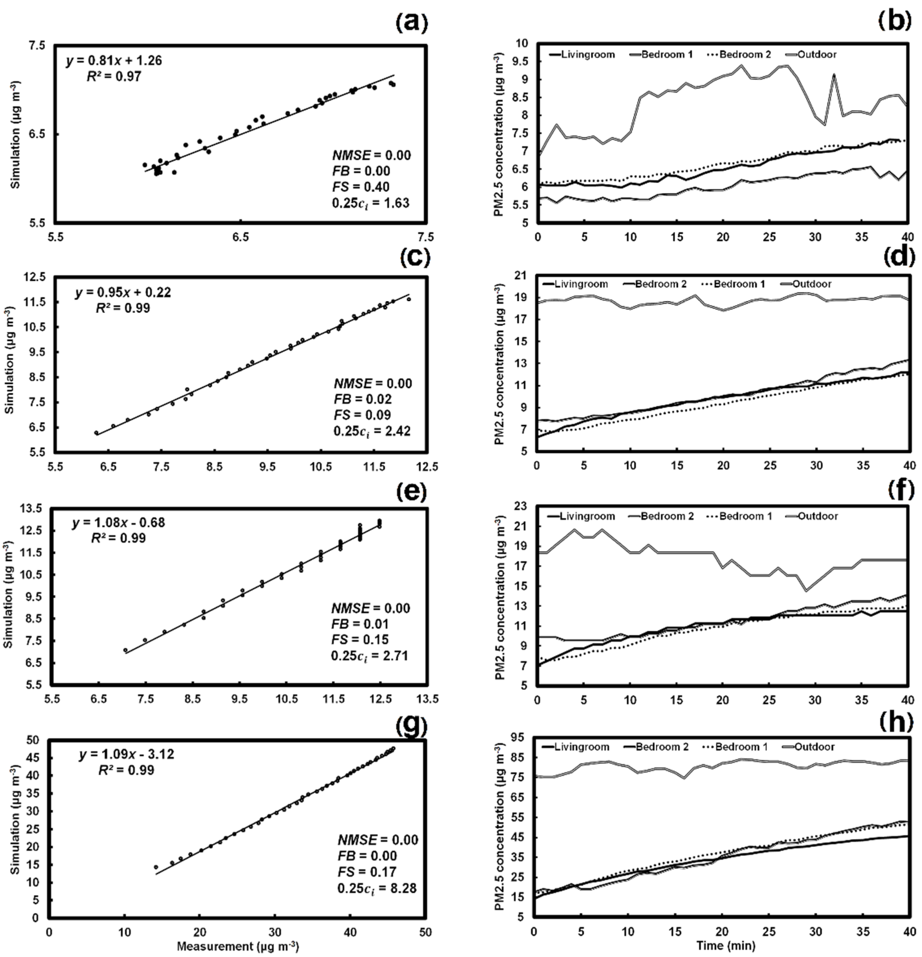
3.1. Indoor PM_2.5 Concentration: Simulation and Measurements

Figure 4a–h present the PM_2.5 concentrations from CONTAM simulations versus measurements from the living room with statistical analysis and measured concentrations in three indoor zones (living room, bedroom 1, and bedroom 2) and outside over a duration related to the air change rate of the room [23] under the 4 Pa depressurization set on different days. The relationships between simulated and measured concentrations are shown in Figure 4a,c,e,g) on 8, 9, 15, and 16 September, respectively. The figures indicate a good agreement between measured and predicted PM_2.5 concentrations from different days, although the variations of fractional bias (FB) of days are seen. There are differences in PM_2.5 change among the three zones (Figure 4b–h), so PM_2.5 concentrations in bedroom 1 were generally a little lower than that of other zones (Figure 4b), although this was true every day, hinting at the influence of external variations, including weather and outdoor PM_2.5 concentrations. Figure 5a–h further compares CONTAM results and measurements and the 3-h observations from the rooms and outdoors under natural conditions, on 11 (a, b), 12 (c, d), 13 (e, f), and 15 (g, h) September. The figures show poorer fits with lower R², compared with the constant pressure set of Figure 4. It is likely to be caused by increased propagation of variable outdoor conditions (e.g., wind speed, indoor–outdoor temperature gradient) under natural ventilation. All data were calibrated using real weather data by using on-site measurement.

Although the statistical analyses show that the agreement between observation and model prediction is not perfect for all cases, it is encouraging to note that most statistical parameters are in the acceptable range, meeting the six criteria of ASTM D5157 Standard Guide. In general, most measured PM_2.5 concentrations of the three indoor zones show similar positive trends in depressurization and natural conditions, thus, it is reasonable to use the average values for estimating the overall deposition rates and penetration factors. As the modeled PM_2.5 concentrations of both sets in different days illustrate an acceptable agreement with the measurement values, the predicted concentrations are well trusted and can be extended to model the variations of PM_2.5 concentrations over longer times.

3.2. Simulating Variability

The coefficient of variation of indoor concentration across four days in different seasons was investigated, by simulating the 24-h indoor PM_2.5 variations under −4 Pa indoor-outdoor pressure difference induced by a blower-door fan and natural conditions in CONTAM. The four months were chosen to include March, June, September, and December representing four seasons and the middle day of each of the months (15th) was selected. All other parameters including deposition rate, penetration factor, flow coefficients, etc., were kept the same.

Figure 6 illustrates the 24-h coefficient of variation for concentration across the single days drawn from each season, and a low and stable coefficient is seen when a constant pressure difference was created over the whole period. While under natural conditions, a large variation is observed, up to ~60% for three zones, six times higher than when the blower-door (modeled as a fan) was in place. The changes of ambient conditions also influence the indoor concentration of neighboring apartments, which further affected the test apartment. Thus, the measurement variation across four seasons can be reduced using the blower-door method in a multistory apartment.

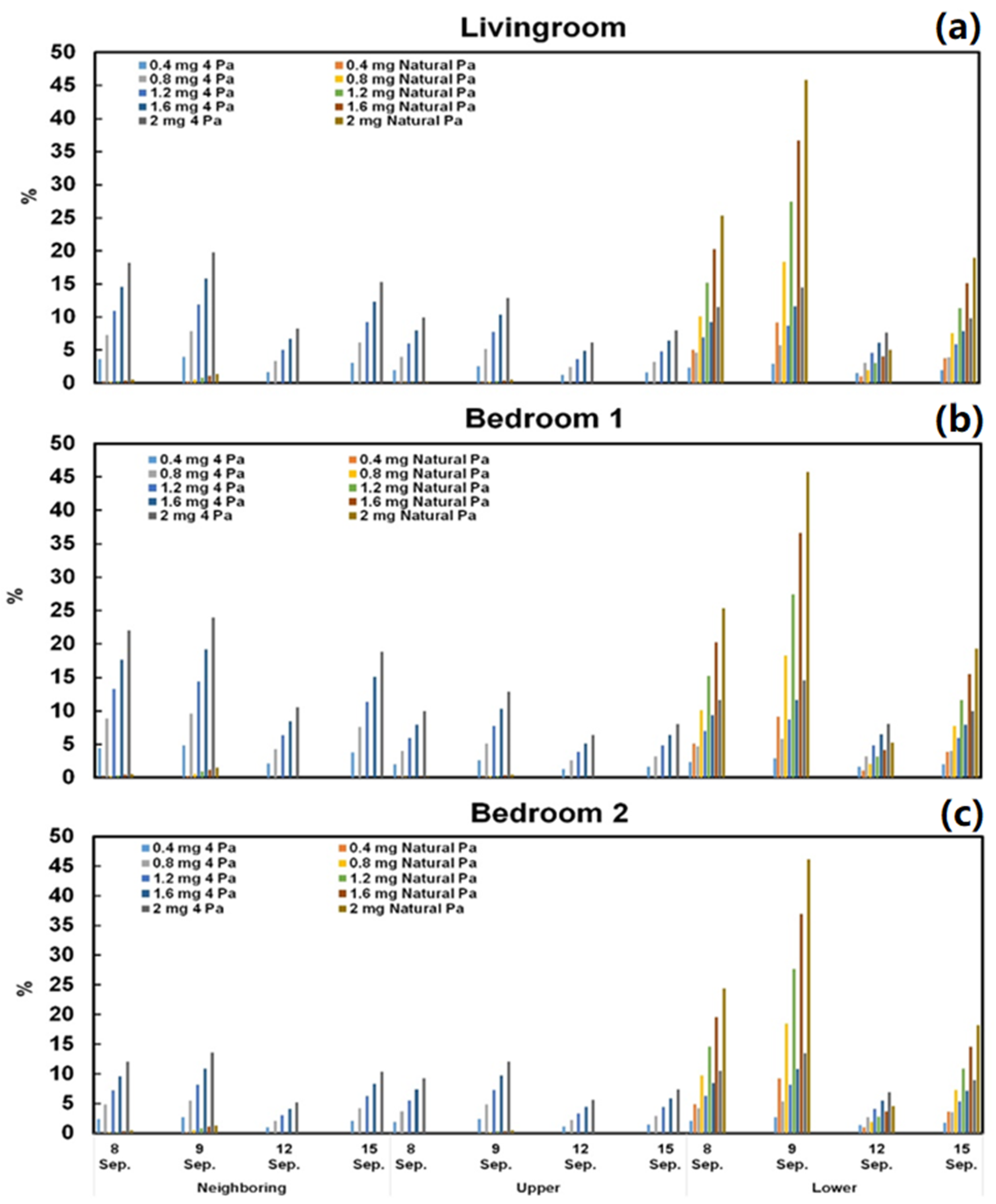
3.3. Effect of Emissions from Adjacent Apartments

Three-hour and 24-h indoor PM_2.5 concentrations over four different periods (8–9; 9–10; 12–13; 15–16 September) were modeled using CONTAM, by changing the emission rates of the three adjacent apartments: (i) opposite neighboring apartments on the same floor, (ii) upper floor, and (iii) lower floor apartments. The four days were selected to cover a relatively wide range of wind speeds as seen in Table 1: 0.49 to 1.41 m s⁻¹. Integration of the PM_2.5 concentration over time was used to represent an accumulated PM_2.5 level. The kitchen was set as the location of PM_2.5 generation. One-hour periods of particle generation with five constant generation rates: 0.4, 0.8, 1.2, 1.6, and 2.0 mg min⁻¹ were used; realistic for PM_2.5 emission rate for different types of cooking [40]. Since outdoor weather conditions are one of the most important influence on indoor particle exchange or accumulation [19,41], outdoor concentrations were not changed when the indoor concentrations were modeled for different days. The simulation of 15 September was selected as an ideal case because measurements and simulations were well correlated (R² = 0.99) under both conditions for all three zones. The 24-h indoor PM_2.5 concentrations from 15–16 September were modeled and the accumulation on different days presented. The penetration factors estimated from indoor and outdoor concentrations during two periods (first three-hour and 24-h) under blower-door conditions were computed based on Equation (3). The error in the estimated penetration factor under different emission rates was compared with those of the no-generation condition, with all other parameters kept the same in the CONTAM model. It reveals the effects of neighboring emission on estimates from the blower-door method.

3.3.1. PM_2.5 Accumulation, Error of Penetration Factor and Window Closure

Window opening is one of the most important controls on indoor pollutant levels [28], but there are few investigations of the effect of windows in adjacent apartments. Figure 7 illustrates the increased percentages of the PM_2.5 accumulating in the three indoor zones at five emission rates in the three adjacent apartments: (a) when all windows were closed or (b) open in opposite neighboring apartments on the same day. Higher generation rates always result in increased percentages of indoor PM_2.5 level for the whole apartment. The increased percentages found when windows are closed are much higher than those for all zones, when windows are open. The highest value is up to 20% for closed windows, but only 0.07% for open windows. It suggests that the indoor PM_2.5 concentration is less influenced by the PM_2.5 generation of neighboring apartments when all windows are open, probably because open windows result in larger air change rates and mean that the increased particle concentration in neighboring apartments disperse outdoors. The resulting PM_2.5 concentrations tend to be similar even when generation rates change.

Figure 7a further shows the percentage increase in PM_2.5 concentrations under two conditions (constant 4 Pa and natural conditions). At 4 Pa, the largest percentage increase is seen in bedroom 1 when the PM_2.5 was generated in the adjacent apartment on the same floor, <20%. Regarding the layout of this building, bedroom 1 is connected directly to the adjacent zones, but the living room is not, revealing the corridor area provides more time for PM_2.5 to dilute and disperse. It further reduces the accumulation in the indoor areas, i.e., there are more air flow paths between test zones and corridor areas, as shown in Figure 3. The larger number of air flow paths, between indoor and adjacent apartments on the same floor, suggests that PM_2.5 would allow easier penetration indoors under a constant indoor-outdoor pressure difference. The lowest increase is seen in bedroom 2, probably because bedroom 2 is not directly or indirectly linked to any adjacent areas and is thus more easily influenced by outdoor variations.

When the blower-door fan was removed, yet PM_2.5 emission rates maintained as in the previous case, concentrations were almost unchanged. However, the greatest increase was observed across all indoor zones when generation sources were located in the apartment on the lower floor, even though there are fewer air flow paths between the two zones, so it is likely to be caused by stack effects. Opening adjacent windows did not cause a strong change of PM_2.5 concentrations, the largest, though small, increase still arises from the lower apartment (<0.07%, as shown in Figure 7b).

Table 3. Penetration factor estimated by modeling indoor concentration and outdoor value under 4 Pa pressure difference with five generation rates during two periods. Cv is the coefficient of variation of the mean.

Time	Sources Location	Neighboring Window Condition	Emission Rate (mg min−1)
			0	0.4	0.8	1.2	1.6	2.0	Mean	Cv (%)
Three hours	Adjacent apartment	Closing	0.86	1.07	1.28	1.49	1.70	1.91	1.39	28.37
		Opening	0.91	0.91	0.91	0.91	0.91	0.91	0.91	0
	Upper apartment	Closing	0.86	1.00	1.14	1.28	1.42	1.56	1.21	21.65
		Opening	0.89	0.89	0.89	0.89	0.89	0.89	0.89	0
	Lower apartment	Closing	0.86	1.02	1.19	1.36	1.53	1.69	1.28	24.53
		Opening	0.89	0.89	0.89	0.89	0.89	0.89	0.89	0
	Mean		0.88	0.96	1.05	1.14	1.22	1.31
	Cv (%)		2.43	7.98	16.57	23.88	30.15	35.52
24 h	Adjacent apartment	Closing	0.87	0.88	0.89	0.9	0.91	0.92	0.90	2.09
		Opening	0.95	0.95	0.95	0.95	0.95	0.95	0.95	0
	Upper apartment	Closing	0.87	0.87	0.88	0.88	0.89	0.89	0.88	1.02
		Opening	0.91	0.91	0.91	0.91	0.91	0.91	0.91	0
	Lower apartment	Closing	0.87	0.88	0.88	0.89	0.89	0.9	0.89	1.19
		Opening	0.92	0.92	0.92	0.92	0.92	0.92	0.92	0
	Mean		0.90	0.90	0.91	0.91	0.91	0.92
	Cv (%)		3.75	3.39	3.03	2.73	2.44	2.27

lists the penetration factor estimated from Equation (3) based on the average of three indoor zones and outdoor PM_2.5 concentrations during two periods (first three-hour and 24 h) under 4 Pa pressure difference on the same day. The penetration factors tend to be similar, with the input value of 0.89 in CONTAM driven from field experiment when there was no emission from neighboring units across all conditions. However, an obvious difference in the estimates can be seen for different emission rates during the two periods. Since the emission of PM_2.5 will cease after an hour, representing an actual cooking period, the three-hour estimates cover a short-time duration, similar to that of the experimental duration, while 24-h embraces a longer time. With windows closed, the penetration factors increase at higher emission rates, and the values are always higher than unity for the three-hour period. The highest average penetration factor for all emission rates is 1.39, when the sources are in the adjacent apartment, where Cv > 28% for the three-hour period. The estimates for the sources coming from upper and lower apartments are only slightly less than those from the adjacent unit, with Cv > 20%. It suggests that the estimated penetration factor has a large variation for different neighboring emission rates over short-time durations. However, the estimates tend to be similar when the testing duration extends to 24 h. All penetration factors are close to 0.89, similar to that with no generation, and a Cv ~ 2% for different emission rates with sources present in the adjacent unit. When the window is open, the estimates of penetration factor are not influenced by neighboring emissions.

The study also reveals that large variation in estimates when the neighboring windows are open or not during the three-hour period. Variation tends to be more obvious at higher emission rates, but the window status does not influence the 24-h duration, with all Cv > 4%. Compared with the three-hour estimates, a 24-h period test provides a more precise and accurate value. The precision and accuracy of the blower-door method could improve estimates of penetration factors because the emitted particles have longer to disperse outdoors or deposit in neighboring interiors.

3.3.2. PM_2.5 Accumulation and the Error of Penetration Factor on Different Days

Figure 8 shows the 24-h percentage increase of PM_2.5 concentration in (a) the living room, (b) bedroom 1 and (c) bedroom 2 on four days, when the sources in adjacent apartments over three levels were changed. The most dramatic increase in PM_2.5 on different days is seen when the PM_2.5 was produced on the lower floor. The highest percentage (>45%) for the three zones, is observed when the lower floor emission rate is 2 mg min⁻¹ (9 September) under natural conditions. The smallest increase from the source below is seen on 12 September, <7%, at 2 mg min⁻¹ under the 4 Pa set. At 4 Pa depressurization, the highest increase is observed when the sources come from the apartment on the same floor across all generation rates. This may result from the large gaps or cracks between adjacent apartments in multistory buildings (e.g., interior doors and windows), compared with the gaps between the ceiling and floor. Under natural conditions, when the sources are on the lower floor apartment, the percentage increase is much larger than the cases where sources are associated with other floors. It suggests that stack effects could be a dominating factor influencing indoor PM_2.5 where sources are below. The assumptions made in assigning the distribution and location of the air gaps will of course influence the relative importance of different transport mechanisms. The accumulation in bedroom 2 tends to be small when the source is from opposite apartments as bedroom 2 is not directly attached to it.

Table 4. Average penetration factor under 4 Pa pressure difference during two periods for four days (8, 9, 12, and 15 September) with five generation rates (0.4; 0.8; 1.2; 1.6; 2 mg min⁻¹). Cv is the coefficient of variation of the mean.

Time	Sources Location		Emission Rate (mg min−1)
			0	0.4	0.8	1.2	1.6	2.0	Mean	Cv (%)
Three hours	Adjacent apartment	Mean	0.85	1.05	1.25	1.45	1.65	1.86	1.35	27.96
		Cv (%)	2.95	6.94	9.28	11.42	12.95	14.01
	Upper apartment	Mean	0.85	0.99	1.14	1.29	1.43	1.58	1.21	22.62
		Cv (%)	2.95	3.62	4.21	4.94	5.01	5.59
	Lower apartment	Mean	0.85	1.01	1.18	1.35	1.52	1.69	1.27	24.86
		Cv (%)	2.95	2.84	3.04	3.22	3.31	3.43
24 h	Adjacent apartment	Mean	0.87	0.88	0.89	0.91	0.92	0.92	0.90	2.15
		Cv (%)	1.44	1.43	1.41	0.64	0.63	0.54
	Upper apartment	Mean	0.87	0.88	0.88	0.89	0.90	0.90	0.89	1.20
		Cv (%)	1.44	1.61	1.43	1.59	1.07	1.28
	Lower apartment	Mean	0.87	0.88	0.89	0.90	0.90	0.91	0.89	1.49
		Cv (%)	1.44	1.43	1.08	1.44	1.28	1.27

lists the average estimated penetration factor at 4 Pa pressure difference during two periods (first three-hour and 24-h) for four days. The coefficient of variation (Cv) shows a positive trend for the three-hour duration under different emission rates, from around 7% at 0.4 mg min⁻¹ to 14% at 2 mg min⁻¹ when the sources are in the adjacent apartment. Variation tends to be lower if the sources are on the units above or below. When the blower-door test time extends to 24 h, the variation decreases to less than 2% for all conditions and the estimates close to the input value in CONTAM that calculated from experimental data. It suggests that a short experimental time can result in an obvious error in the blower-door estimates due to the variation of neighboring emissions and weather conditions. Increasing the experimental measurement time could also improve the precision and accuracy regarding the error in different days.

3.4. A Proposed Experimental Method for Estimating the Distribution of Airflow Paths

It is not always easy to gain long-term access to apartments to conduct extended experiments, so short experiments can bias estimates because of fluctuating sources from neighboring apartments. This means that the precision and accuracy of the blower-door method for estimating PM_2.5 penetration factors using only outdoor concentration is potentially reduced. In this section, a multi-blower door method is proposed to isolate parts of adjacent areas when estimating air change rate in terms of indoor–outdoor transfer. The idea is to create similar pressure differences between zones so eliminating the air exchange. Strictly speaking, Equations (2) and (3) are only correct in the absence of airflow between inter-unit areas. Considering the effects of neighboring apartments, Equation (2) can be rearranged, assuming the deposition rate is the same for the whole apartment:

$$\frac{d{c}_i}{dt}=P_o{m}_o{k}_{ACH,\Delta p}{c}_o+P_{ad}{m}_{ad}{k}_{ACH,\Delta p}{c}_{ad}+P_{cor}{m}_{cor}{k}_{ACH,\Delta p}{c}_{cor}-\left(k_{ACH,\Delta p}+v_{\Delta p}\right)c_i$$

(7)

where $P_o$, $P_{ad}$, $P_{cor}$ are the penetration factors of outside, adjacent units and corridor areas respectively; $m_o$, $m_{ad}$, $m_{cor}$ is air change rate as a proportion of that outside, adjacent units, and corridor, respectively; $c_{ad}$ is the concentration of PM_2.5 of adjacent units and $c_{cor}$ is the concentration in the corridor. More specifically, the airflow and contaminant transfer from upper, lower, and horizontally positioned adjacent units, can be expressed as:

$$m_{ad}{c}_{ad}=m_{up}{c}_{up}+m_{lo}{c}_{lo}+m_{ho}{c}_{ho}$$

(8)

where $m_{up}$, $m_{lo}$, $m_{ho}$ are air change rate proportions of the upper, lower floor of unit and horizontal adjacent unit respectively; $c_{up}$, $c_{lo}$, $c_{ho}$ the concentration of PM_2.5 for the upper, lower and horizontal units. Assuming all penetration factors are the same, solving Equation (7) when it is not the steady-state condition by a backward differential scheme, gives indoor PM_2.5 as a function of time:

$$c_i\left(t\right)=P{k}_{ACH,\Delta p}\left[m_o{c}_o\left(t-1\right)+m_{up}{c}_{up}\left(t-1\right)+m_{lo}{c}_{lo}\left(t-1\right)+m_{ho}{c}_{ho}\left(t-1\right)+ m_{cor}{c}_{cor}\left(t-1\right)\right]\Delta t+\left(1-\left(k_{ACH,\Delta p}+v_{\Delta p}\right)\Delta t\right)c_i\left(t-1\right)$$

(9)

Equation (9) combines the relevant factors including upper, lower, horizontal adjacent units, and the external environment under minimum ventilation mode (assuming windows closed, and all holes sealed), and the average indoor concentrations of all zones were assumed to reflect the trend of the whole apartment. As shown in Figure 3, the lift areas of different floors are phantom zones along with the stairwells. Thus, it is hard to create the same pressure difference between stairwell/lift zones and other areas. The gaps and cracks between all zones in the test room and stairwell/lift zones should be sealed because the contribution; those gaps is less than 5%, based on the modeling results. Based on the normal blower-door test, another blower-door fan (Fan 2) is installed in four positions sequentially to isolate gaps between the adjacent zones and test apartment, as shown in Figure 9. Thus, four additional tests should be carried out after measuring the air change rate of the whole test apartment:

(i) Installing one more blower-door fan (Fan 2) in the same position with the original one in the upper or lower floor apartments. Then setting the same pressure difference between indoors and outdoors for the two apartments and testing the air change rates of two apartments simultaneously. In this case, most air cannot be blown into the test apartment from upper or lower floor areas, thus, the difference in air change rate between two apartments can estimate the air change rate of the connected areas. It should be noted that this consists of two tests, one for the upper floor and another for the lower floor. After this the air change rate from ceiling and floor can be evaluated separately.

(ii) The second fan would then be moved to the door of bedroom 2 of the adjacent apartment and subsequently to the front door of the living room of the neighboring apartment, which connects to the corridor area on the same floor, as shown in Figure 9. Creating the same pressure difference, allows the difference in air change rate to be determined. Thus, the air change rate from corridor to living room and that from the area adjacent to bedroom 1 can be calculated.

Table 5. Air change rate proportion of four adjacent areas and outside.

Isolated Zone	Air Change Rate Proportion (m)		Absolute Difference	Percentage (%) (100x Absolute Difference/Calculated Value)
	Calculated Value	Simulated Value
Horizontal adjacent apartment $\left({\mathit{n}}_{\mathit{h}\mathit{o}}\right)$	0.068	0.064	0.004	6
Upper floor apartment $\left({\mathit{n}}_{\mathit{u}\mathit{p}}\right)$	0.065	0.062	0.003	5
Lower floor apartment $\left({\mathit{n}}_{\mathit{l}\mathit{o}}\right)$	0.053	0.056	0.003	6
Corridor area $\left({\mathit{n}}_{\mathit{c}\mathit{o}\mathit{r}}\right)$	0.105	0.105	0.000	0
Outside $\left({\mathit{n}}_{\mathit{o}}\right)$	0.709	0.713	0.003	0

compares the proportional air change rate of the upper floor, lower floor, corridor, and adjacent area, which were computed by the multi blower-door method of Equation (9) and the CONTAM simulation. Both values show a similar percentage for these areas, with the percentage difference less than 6%. Figure 10 gives an example of the relationship between PM_2.5 concentrations estimated from Equation (9) and the simulated concentrations at 4 Pa. A slope of 0.99, intercept of 0.13 and R² of 0.99 were seen, with both biases only 0.01, suggesting the analytical results have a relatively good agreement with the model. The multi blower-door method is an improvement on the simple blower-door method, reducing the effects of adjacent areas on indoor PM_2.5 variations. It is believed that using the air change rate from outside only can greatly improve the precision for the blower-door method in estimating the PM_2.5 penetration factor.

4. Conclusions

The variation of indoor PM_2.5 concentration over time with respect to fluctuating sources in adjacent apartments and different building layouts was simulated in the present work. It predicted indoor PM_2.5 concentrations under variable weather conditions and investigated the effects of sources from neighboring areas on the accumulation of PM_2.5 to ascertain the influence of changing environments on estimating particle penetration factors. Both CONTAM simulations and experiments were performed for a residential test building using two methods: the blower-door and traditional decay-rebound method. The results show that the CONTAM modeling has good agreement with the experimental results using both methods, so the model is to be trusted and suitable for exploring scenarios with different sources of PM_2.5. Assuming outside concentration is not influenced by the emission of neighboring units, a higher emission rate of PM_2.5 in neighboring apartments always resulted in higher accumulation of indoor PM_2.5 in the test apartment. When a constant pressure difference was created, the sources in the adjacent apartment on the same floor had a bigger effect on indoor accumulation, due to the larger air change rate; an important factor that can increase error in the estimates. However, when the decay and rebound method is used, under natural conditions, the emission of PM_2.5 from neighboring apartments on lower floors significantly effects the concentration in the test apartment because of the stack effect. Although the blower-door method can reduce the variation of deposition rate and penetration factor estimates compared with the natural conditions, the effects of adjacent apartments should be considered. Emission from neighboring units is an important factor that influences the precision and accuracy of the estimated penetration factor during short measuring times. Opening the window in the source apartment and extending the measuring time could reduce the error of the estimates. Simulation suggests that using a multi-blower system to remove ingress from neighboring apartments could also reduce the variation in estimates of penetration factor, which might be more useful for those short time measurements (e.g., less than three hours). The work highlights the effect of transfer of air between apartments on indoor air quality.

References

1. Klepeis, N.E.; Neilson, W.C.; Ott, W.R.; Robinson, J.P.; Tsang, A.M.; Switzer, P.; Behar, J.V.; Hern, S.C.; Englemann, W.H. The national human activity pattern survey (NHAPS): A resource for assessing exposure to environmental pollutants. J. Exp. Anal. Environ. Epidemiol. 2001, 11, 231–252. [Google Scholar] [CrossRef] [PubMed] [Green Version]
2. Samuel, A.A.; Strachan, P. An Integrated Approach to Indoor Contaminant Modeling. HVAC&R Res. 2006, 12 (Suppl. S1), 599–619. [Google Scholar]
3. ASHRAE. ASHRAE Handbook—2009 Fundamentals; ASHRAE: Atlanta, GA, USA, 2009. [Google Scholar]
4. Lai, Y.; Ridley, I.A.; Brimblecombe, P. Air Change in Low and High-Rise Apartments. Urban Sci. 2020, 4, 25. [Google Scholar] [CrossRef]
5. Mao, J.C.; Gao, N.P. The airborne transmission of infection between flats in high-rise residential buildings: A review. Build. Environ. 2005, 94, 516–531. [Google Scholar] [CrossRef] [PubMed]
6. Yu, I.T.; Li, Y.; Wong, T.W.; Tam, W.; Chan, A.T.; Lee, J.H.; Ho, T. Evidence of airborne transmission of the severe acute respiratory syndrome virus. N. Engl. J. Med. 2004, 350, 1731–1739. [Google Scholar] [CrossRef] [PubMed] [Green Version]
7. Yeung, K.H.; Yu, I.T.S. Possible meteorological influence on the severe acute respiratory syndrome (SARS) community outbreak at Amoy Gardens. J. Environ. Health 2007, 70, 39–46. [Google Scholar]
8. Health, Welfare & Food Bureau. SARS Bulletin 28 May 2003. In Government of the Hong Kong Special Administrative Region; 2012. Available online: http://www.info.gov.hk/info/sars/bulletin/bulletin0528e.pdf (accessed on 24 December 2020).
9. Liu, X.P.; Niu, J.L.; Perino, M.; Heiselberg, P. Numerical simulation of inter-flat air cross contamination under the condition of single-sided natural ventilation. J. Build. Perform. Simul. 2008, 1, 133–147. [Google Scholar] [CrossRef]
10. Wu, Y.; Niu, J.L. Assessment of mechanical exhaust in preventing vertical cross-household infections associated with single-sided ventilation. Build. Environ. 2016, 105, 307–316. [Google Scholar] [CrossRef]
11. Wang, J.H.; Wang, S.G.; Zhang, T.F.; Battaglia, F. Assessment of single-sided natural ventilation driven by buoyancy forces through variable window configurations. Energy Build. 2017, 139, 762–779. [Google Scholar] [CrossRef]
12. Mu, D.; Gao, N.P.; Zhu, T. Wind tunnel tests of inter-flat pollutant transmission characteristics in a rectangular multi-storey residential building, part A: Effect of wind direction. Build. Environ. 2016, 108, 159–170. [Google Scholar] [CrossRef]
13. Mu, D.; Gao, N.P.; Zhu, T. Wind tunnel tests of inter-flat pollutant transmission characteristics in a rectangular multi-storey residential building, part B: Effect of source location. Build. Environ. 2017, 114, 281–292. [Google Scholar] [CrossRef] [PubMed]
14. Mao, J.C.; Yang, W.W.; Gao, N.P. The transport of gaseous pollutants due to stack and wind effect in high-rise residential buildings. Build. Environ. 2015, 94, 543–557. [Google Scholar] [CrossRef]
15. Wang, L.; Dols, W.S.; Chen, Q. Using CFD Capabilities of CONTAM 3.0 for Simulating Airflow and Contaminant Transport in and around Buildings. HVAC&R Res. 2010, 16, 749–763. [Google Scholar]
16. Argyropoulos, C.D.; Hassan, H.; Kumar, P.; Kakosimos, K.E. Measurements and modelling of particulate matter building ingress during a severe dust storm event. Build. Environ. 2020, 167, 106441. [Google Scholar] [CrossRef]
17. Underhill, J.; Dols, W.S.; Lee, S.K.; Fabian, M.P.; Levy, J.I. Quantifying the impact of housing interventions on indoor air quality and energy consumption using coupled simulation models. J. Expo. Sci. Environ. Epidemiol. 2020, 30, 436–447. [Google Scholar] [CrossRef]
18. Zhu, S.; Jenkins, S.; Addo, K.; Heidarinejad, M.; Romo, S.A.; Layne, A.; Ehizibolo, J.; Dalgo, D.; Mattise, N.W.; Hong, F.; et al. Ventilation and laboratory confirmed acute respiratory infection (ARI) rates in college residence halls in College Park, Maryland. Environ. Int. 2020, 137, 105537. [Google Scholar] [CrossRef]
19. Lai, Y.; Brimblecombe, P.; Ridley, I.A. Estimating PM2.5 penetration factors and deposition rates in a dwelling using a combined blower-door test. In Proceedings of the Indoor Air 2018—15th International Conference of the Society of Indoor Air Quality and Climate, Philadelphia, PA, USA, 22 July–27 July 2018. Paper No. 165. [Google Scholar]
20. Nabinger, S.; Persily, A. Impacts of airtightening retrofits on ventilation rates and energy consumption in a manufactured home. Energy Build. 2011, 43, 3059–3067. [Google Scholar] [CrossRef]
21. Sherman, M.H.; Chan, R. Building air tightness: Research and practice. In Lawrence Berkeley National Laboratory Report No. LBNL 53356; Lawrence Berkeley National Laboratory: Berkeley, CA, USA, 2004. [Google Scholar]
22. Zhu, Y.; Smith, T.J.; Davis, M.E.; Levy, J.I.; Herrick, R.; Jiang, J. Comparing Gravimetric and Real-Time Sampling of PM2.5 Concentrations inside Truck Cabins. J. Occup. Environ. Hyg. 2011, 8, 662–672. [Google Scholar] [CrossRef] [Green Version]
23. Lai, Y.; Ridley, I.A.; Brimblecombe, P. Blower-door estimates of PM2.5 deposition rates and penetration factors in an idealised room. Indoor Built Environ. 2020. [Google Scholar] [CrossRef]
24. Thatcher, T.L.; Lunden, M.M.; Revzan, K.L.; Sextro, R.G.; Brown, N.J. A concentration rebound method for measuring particle penetration and deposition in the indoor environment. Aerosol Sci. Technol. 2003, 37, 847–864. [Google Scholar] [CrossRef]
25. Rim, D.; Wallace, L.; Persily, A. Infiltration of outdoor ultrafine particles into a test house. Environ. Sci. Technol. 2010, 44, 5908–5913. [Google Scholar] [CrossRef] [PubMed]
26. Stephens, B.; Siegel, J.A. Penetration of ambient submicron particles into single-family residences and associations with building characteristics. Indoor Air. 2012, 22, 501–513. [Google Scholar] [CrossRef] [PubMed]
27. Hu, B.; Freihaut, J.D.; Bahnfleth, W.P.; Aumpansub, P.; Thran, B. Modeling Particle Dispersion under Human Activity Disturbance in a Multizone Indoor Environment. J. Architect. Eng. 2007, 13, 187. [Google Scholar] [CrossRef]
28. Rim, D.; Persily, A.; Emmerich, S.; Dols, W.S.; Wallace, L. Multi-zone modeling of size-resolved outdoor ultrafine particle entry into a test house. Atmos. Environ. 2013, 69, 219–230. [Google Scholar] [CrossRef]
29. Dols, W.S.; Emmerich, S.J.; Polidoro, B.J. Coupling the multizone airflow and contaminant transport software CONTAM with EnergyPlus using co-simulation. Build. Simul. 2016, 9, 469–479. [Google Scholar] [CrossRef] [PubMed]
30. Dols, W.S.; Polidoro, B.J. NIST Technical Note 1887: CONTAM User Guide and Program Documentation; National Institute of Standards and Technology: Gaithersburg, MD, USA, 2015. [Google Scholar]
31. Liu, F.; Gong, N.; Yan, Z.J. Opening Flow Coefficient and its Effect on Fire Smoke Flow. J. Chongqing Jianzhu Univ. 2000, 22, 86–92. [Google Scholar]
32. Swami, M.V.; Chandra, S. Procedures for calculating natural ventilation airflow rates in buildings. In Work Performed for ASHRAE Research Project 448-RP; Florida Solar Energy Center: Cocoa, FL, USA, 1987. [Google Scholar]
33. Ng, L.; Musser, A.; Persily, A.K.; Emmerich, S.J. Multizone airflow models for calculating infiltration rates in commercial reference buildings. Energy Build. 2013, 58, 11–18. [Google Scholar] [CrossRef]
34. Abt, E.; Suh, H.H.; Catalano, P.; Koutrakis, P. Relative contribution of outdoor and indoor particle sources to indoor concentrations. Environ. Sci. Technol. 2000, 34, 3579–3587. [Google Scholar] [CrossRef]
35. Wallace, L.; Emmerich, S.J.; Howard-Reed, C. Effect of central fans and in-duct filters on deposition rates of ultrafine and fine particles in an occupied townhouse. Atmos. Environ. 2004, 38, 405–413. [Google Scholar] [CrossRef]
36. He, C.; Morawska, L.; Gilbert, D. Particle deposition rates in residential houses. Atmos. Environ. 2005, 39, 3891–3899. [Google Scholar] [CrossRef] [Green Version]
37. Long, C.M.; Suh, H.H.; Catalano, P.J.; Koutrakis, P. Using time- and size-resolved particulate data to quantify indoor penetration and deposition behaviour. Environ. Sci. Technol. 2001, 35, 2089–2099. [Google Scholar] [CrossRef] [PubMed]
38. ASHRAE. ASHRAE Handbook—2005 Fundamentals; ASHRAE: Atlanta, GA, USA, 2005. [Google Scholar]
39. ASTM D5157-19; Standard Guide for Statistical Evaluation of Indoor Air Quality Models; ASTM International: West Conshohocken, PA, USA, 2019.
40. Hu, T.; Singer, B.C.; Logue, J.M. Compilation of published PM2.5 Emission Rates for cooking, candles and incense for use in Modeling of exposures in residences. In Lawrence Berkeley National Lab (LBNL) Report No. LBNL 53356; Lawrence Berkeley National Laboratory: Berkeley, CA, USA, 2012. [Google Scholar]
41. Lai, A.C.K. Particle deposition indoors: A review. Indoor Air 2002, 12, 211–214. [Google Scholar] [CrossRef] [PubMed]
Figure 1. (a) The multistory apartment building; (b) floor layout; identical on each floor.
Urbansci 05 00002 g001
Figure 2. Calibration between fine particulate matter (PM2.5) monitor in living room and bedroom 1 (a) and in living room and bedroom 2 (b).
Urbansci 05 00002 g002
Figure 3. Graphic interface for each floor of the multistory building, where the blower-door fan was only installed in the test apartment.
Urbansci 05 00002 g003
Figure 4. PM2.5 concentration of CONTAM simulation and measurement in the living room (a,c,e,g) and the measured PM2.5 concentration (b,d,f,h) in the living room and bedrooms 1 and 2, and outside under the 4 Pa depressurization set on four different days: 8 September (a,b), 9 September (c,d), 15 September (e,f), and 16 September (g,h). The y is the simulation, and x is the measurement.
Urbansci 05 00002 g004
Figure 5. PM2.5 concentration of CONTAM simulation and measurement in the living room and the measured PM2.5 concentration in four places (living room, bedroom 1, bedroom 2, and outside) under three-hour natural conditions on four different days: 11 September (a,b), 12 September (c,d), 13 September (e,f), and 15 September (g,h), respectively. The y is the simulation, and x is the measurement.
Urbansci 05 00002 g005
Figure 6. Coefficient of variation (%) of indoor PM2.5 concentration in the living room (a), bedroom 1 (b) and bedroom 2 (c) under two conditions (−4 Pa pressure difference induced by fan and natural conditions) across four days in different seasons.
Urbansci 05 00002 g006
Figure 7. The percentage increase in PM2.5 accumulation in the three indoor zones at five generation rates (0.4; 0.8; 1.2; 1.6; 2 mg min−1) from three adjacent apartments: Opposite neighboring (Nei), Upper and Lower apartments, under two conditions (4 Pa depressurization and natural conditions), with windows closed (a) and opened (b) in neighboring apartments.
Urbansci 05 00002 g007
Figure 8. The percentage increase of PM2.5 concentration in living room (a), bedroom 1 (b) and bedroom 2 (c) in four days (8, 9, 12, and 15 September) with five generation rates (0.4; 0.8; 1.2; 1.6; 2 mg min−1) on the three floors (neighboring, upper, and lower apartments) based on two conditions.
Urbansci 05 00002 g008
Figure 9. The places of Fan 2 for proposed experimental method.
Urbansci 05 00002 g009
Figure 10. An example of the relationship between PM2.5 concentrations estimated from Equation 9 and the simulated concentrations at 4 Pa depressurization.
Urbansci 05 00002 g010