Optimal D-STATCOM Operation in Power Distribution Systems to Minimize Energy Losses and CO₂ Emissions: A Master–Slave Methodology Based on Metaheuristic Techniques

Abstract

In this paper, we address the problem of intelligent operation of Distribution Static Synchronous Compensators (D-STATCOMs) in power distribution systems to reduce energy losses and CO₂ emissions while improving system operating conditions. In addition, we consider the entire set of constraints inherent in the operation of such networks in an environment with D-STATCOMs. To solve such a problem, we used three master–slave methodologies based on sequential programming methods. In the proposed methodologies, the master stage solves the problem of intelligent D-STATCOM operation using the continuous versions of the Monte Carlo (MC) method, the population-based genetic algorithm (PGA), and the Particle Swarm Optimizer (PSO). The slave stage, for its part, evaluates the solutions proposed by the algorithms to determine their impact on the objective functions and constraints representing the problem. This is accomplished by running an Hourly Power Flow (HPF) based on the method of successive approximations. As test scenarios, we employed the 33- and 69-node radial test systems, considering data on power demand and CO₂ emissions reported for the city of Medellín in Colombia (as documented in the literature). Furthermore, a test system was adapted in this work to the demand characteristics of a feeder located in the city of Talca in Chile. This adaptation involved adjusting the conductors and voltage limits to include a test system with variations in power demand due to seasonal changes throughout the year (spring, winter, autumn, and summer). Demand curves were obtained by analyzing data reported by the local network operator, i.e., Compañía General de Electricidad. To assess the robustness and performance of the proposed optimization approach, each scenario was simulated 100 times. The evaluation metrics included average solution quality, standard deviation, and repeatability. Across all scenarios, the PGA consistently outperformed the other methods tested. Specifically, in the 33-node system, the PGA achieved a 24.646% reduction in energy losses and a 0.9109% reduction in CO₂ emissions compared to the base case. In the 69-node system, reductions reached 26.0823% in energy losses and 0.9784% in CO₂ emissions compared to the base case. Notably, in the case of the Talca feeder—particularly during summer, the most demanding season—the PGA yielded the most significant improvements, reducing energy losses by 33.4902% and CO₂ emissions by 1.2805%. Additionally, an uncertainty analysis was conducted to validate the effectiveness and robustness of the proposed optimization methodology under realistic operating variability. A total of 100 randomized demand profiles for both active and reactive power were evaluated. The results demonstrated the scalability and consistent performance of the proposed strategy, confirming its effectiveness under diverse and practical operating conditions.

1. Introduction

1.1. Problem Description

Power distribution companies face increasing challenges when it comes to expanding and operating their electrical networks. This situation is primarily due to two factors: (i) the constant growth in power demand and (ii) the integration of new energy generation and storage technologies, such as solar and wind generation systems and battery energy storage systems [1]. Additionally, because of their topologies, power distribution systems (PDSs) experience high energy losses [2] and significant emissions resulting from the use of conventional fossil fuel sources.

To address these challenges, power companies have adopted a variety of strategies aimed at minimizing energy losses and reducing the environmental impact associated with network operation. These strategies include the optimal integration and operation of distributed generation (DG) units in power systems [3], network reconfiguration [4], the optimal integration and operation of reactive power compensation devices in electrical networks [5], and the hybridization of renewable energy sources by incorporating traditional energy storage systems, with optimized charge and discharge control strategies to improve system reliability and energy efficiency [6,7], among others [8]. Among these options, DG has emerged as an attractive solution to meet demand at lower costs. However, DG resources are not available in all power systems. In addition, regions where DG is used are experiencing overgeneration issues during peak sun or wind hours (depending on the resource being employed), leading to negative effects on the network, which are mitigated by reducing renewable energy generation [9].

Another alternative for minimizing energy losses involves reconfiguring electrical distribution networks. This alternative, nonetheless, requires extensive system-wide studies and tests, including a reconsideration of lines and protection systems and analyses of line loadability and voltage [1,10]. Yet, the reductions achieved by these methods are limited when compared to power injection from distributed energy resources.

A further option is the integration of reactive power compensation equipment into electrical networks, such as capacitor banks and reactive power compensation devices. This approach has been extensively explored in transmission systems [11] and has proven to be effective in reducing energy losses, costs, and emissions [12]. It has also been considered for PDSs [13], with an emphasis on the integration of capacitor banks and Distribution Static Synchronous Compensators (D-STATCOMs) [1,14]. Although integrating capacitor banks are the most cost-effective alternative, they are unable to adapt to the dynamic requirements of networks and eventually become obsolete as demand grows and changes. In contrast, D-STATCOMs allow for power level adjustments within a minimum and maximum range to adapt to demand fluctuations while improving system voltage profiles and line correction levels [15].

In simplified terms, a D-STATCOM consists of a voltage source converter, a capacitor that acts as a filter, and an inductance that enables the injection of reactive power into the distribution network [16]. The integration and operation of D-STATCOMs in power distribution systems (PDSs) have gained increasing attention in recent years. Unlike distributed renewable energy resources, which exhibit power variability due to weather conditions, D-STATCOMs provide a controllable and reliable source of reactive power. This allows them to operate consistently at the desired power level, offering greater predictability and flexibility to system operators [14].

Over the past decade, research has primarily focused on the optimal placement and sizing of D-STATCOMs, key aspects for long-term network planning. However, their intelligent operation under real-time and dynamic conditions remains a relatively underexplored area that demands further investigation [12]. Most existing studies emphasize the dynamic behavior of these devices from a power electronics perspective [17,18], yet few address their role in steady-state energy management. Once deployed, D-STATCOMs must adapt to daily variations in active and reactive power demand while maintaining voltage profiles and current levels within operational limits.

Although STATCOMs and D-STATCOMs share the same fundamental principle, using a VSC to exchange reactive power with the network, their practical applications differ [19]. In high-voltage transmission systems, STATCOMs can both inject and absorb reactive power to support system-wide voltage stability. In contrast, D-STATCOMs are typically used in medium- and low-voltage distribution networks, where they primarily inject reactive power to regulate local voltages and reduce losses.

While the underlying technology is the same, the operational requirements differ significantly. Distribution systems are more sensitive to voltage fluctuations due to frequent and unpredictable changes in demand and distributed generation. As a result, D-STATCOMs in these networks require more dynamic and responsive control strategies. Despite this need, the intelligent and adaptive operation of D-STATCOMs under realistic, steady-state conditions has received limited attention and validation in the literature.

To address this gap, the present study proposes and evaluates a methodology focused on the intelligent energy management of D-STATCOMs in actual distribution system scenarios. The objective is to demonstrate how such a strategy can improve the technical and environmental performance of the network, even in the absence of distributed generation or under high-curtailment conditions.

1.2. State of the Art

Given the growing need to promote strategies for the intelligent operation of D-STATCOMs in distribution networks, this paper focuses on addressing this issue, considering the energy demand behavior of PDSs during a typical day of operation. In reviewing the existing literature on the matter, we highlight the contributions made by the authors of [20], who addressed the problem of optimal integration and operation of D-STATCOMs, with the ultimate goal of reducing energy losses and operating and investment costs. Their proposed mathematical model included active and reactive power demand curves. To solve such a problem, the authors employed the vortex search algorithm, whose performance was validated using the 33- and 69-node test systems. Its results were compared to those of other methodologies reported in the literature, demonstrating its effectiveness in terms of solution quality and processing times. However, since current-carrying capacity was not taken into account in the proposed mathematical formulation, the provided solutions are not accurate representations of the actual operational state of PDSs. Additionally, the authors assumed a constant power injection by the D-STATCOMs, limiting their ability to improve the network’s operating conditions.

In [21], the problem of optimal integration and operation of D-STATCOMs and distributed generators in PDSs was solved using the gravitational search algorithm, with the aim of reducing energy losses. The proposed solution methodology was validated on the 33-node test system, proving its effectiveness in lowering energy losses under different operational scenarios. Nevertheless, the authors did not compare its results with those of other methodologies documented in the literature, nor did they analyze the average solution and required processing times, which are vital aspects for determining the effectiveness of the proposed solutions.

In a similar vein, the authors of [14] suggested using the Particle Swarm Optimizer (PSO) to optimally locate, integrate, and operate D-STATCOMs in power distribution networks. As test scenarios, they employed the 33- and 69-node test systems with variable demand curves. The proposed methodology was compared to the following five optimization methods that use commercial software and sequential programming: the BONMIN solver from the General Algebraic Modeling System (GAMS), the Chu and Beasley genetic algorithm, Newton’s metaheuristic algorithm, the vortex search algorithm, and the generalized normal distribution optimization algorithm [22,23].

In an effort to reduce power losses and improve voltage profiles, the authors of [24] employed the Ebola optimization search algorithm to optimally integrate and operate D-STATCOMs in PDSs. The proposed methodology was validated on the 69-node test system, and its results were compared to those of a genetic algorithm and the PSO. The findings demonstrated the effectiveness of the proposed methodology. Nonetheless, the authors did not consider current limits for the lines or analyze the standard deviation of the obtained solutions and the required processing times.

From the studies described above, it is evident that the current research focus in the field is primarily concentrated on the optimal location and sizing D-STATCOMs in electrical networks. However, from an operational perspective, we mostly found contributions in the realm of power electronics and control, as in [25]. In this study, the authors presented a control strategy for injecting reactive power from a D-STATCOM to the grid representing an electrical network. Nevertheless, this approach neglects the network’s multi-nodal mode and its electrical effects. Similarly, in [26], an energy management strategy was proposed for a D-STATCOM connected to a network. Its goal is to ensure proper operation under steady-state conditions, respecting the desired voltage levels and powers. Nonetheless, like the previous approach, this strategy does not take into account the network’s topology and solely focuses on the primary control of the device.

Although various contributions have been made in the past few decades regarding D-STATCOM operation, we found no studies addressing the intelligent operation of these devices in electrical networks. Such a focus is paramount for improving a system’s operating conditions while adhering to the different voltage and current constraints inherent to PDS operation. In fact, this is a current requirement of network operators because changes in the consumption of both active and reactive power necessitate restructuring the reactive power dispatch of D-STATCOMs. The aim is, thus, to build an adaptable and robust system that enhances a network’s operating conditions and ensures that the technical constraints of the network and the devices are respected.

1.3. Research Focus, Key Contributions, and Scope

Building on the contributions in the specialized literature concerning the optimal integration and sizing of D-STATCOMs in PDSs and driven by the identified operational needs, this paper presents a methodology for the intelligent operation of D-STATCOMs in PDSs aimed at reducing energy losses and CO₂ emissions.

This study focuses on the steady-state operation of D-STATCOMs in power distribution systems, assuming normal operating conditions without the occurrence of short-circuit faults or transient events. As such, stability aspects typically associated with transmission-level STATCOMs, such as short-term voltage support or transient stability improvement during faults, are not considered in the proposed operational model. These functions are highly relevant in the context of planning and protection coordination, particularly in systems with synchronous generation [27,28]. However, in distribution systems where D-STATCOMs are primarily deployed to regulate voltage and reduce losses under standard operating scenarios, steady-state analysis remains the most practical and widely adopted approach.

While the majority of studies involving D-STATCOMs focus on planning tasks, such as optimal placement and sizing, this work concentrates on operational optimization. In particular, it addresses the main technical motivation for the injection of reactive power in distribution systems: reducing power losses [29]. In addition to this primary objective, the methodology also considers the environmental impact by including CO₂ emissions as a second optimization criterion, offering a broader perspective on the technical and ecological benefits of D-STATCOM operation.

Although the importance of economic assessments, such as cost–benefit analysis and investment planning, is fully recognized, these aspects were intentionally excluded from the scope of this study. This decision was guided by a review of the relevant literature, which shows that economic modeling is most often associated with the planning stage. In contrast, operational studies tend to focus on technical performance metrics, particularly those related to power quality and system efficiency.

Given the aim of this research to develop a replicable and generalizable strategy for real-world deployment, the proposed model was designed using universally measurable indicators such as energy losses and emissions. Nonetheless, the integration of economic criteria is acknowledged as a valuable extension, and it is considered a relevant direction for future research.

This methodology operates on a master–slave architecture, where the master stage proposes power dispatch configurations for various D-STATCOMs installed in the network, while the slave stage employs an Hourly Power Flow (HPF) to evaluate the objective functions of the solutions offered by the master stage, as well as the constraints of the problem. To that end, the master stage uses three optimization strategies: the Monte Carlo (MC) method, a continuous version of the population-based genetic algorithm (PGA), and the PSO. The choice of these methodologies was grounded in their high effectiveness in addressing power dispatch problems in PDSs for other distributed energy resources [30,31]. The slave stage, for its part, applies an HPF based on the method of successive approximations—a method known for its high efficiency in terms of convergence and processing times [14].

From a practical implementation standpoint, this study adopts metaheuristic optimization techniques due to their flexibility, ease of deployment, and independence from commercial solvers [32]. These characteristics provide significant advantages for real-world applications, particularly in operational environments where access to proprietary software is limited or cost-prohibitive. In contrast to mathematical programming approaches, which often require strict problem formulations and specialized solvers, metaheuristic algorithms can be implemented across diverse computational platforms and are well-suited to handle the nonlinear, non-convex nature of the D-STATCOM operation problem [33]. While these techniques do not guarantee global optimality, the results obtained in this work demonstrate their ability to consistently generate high-quality, repeatable solutions when properly tuned. This modeling choice is consistent with the overall objective of the study: to propose a low-complexity, replicable, and effective optimization strategy for the intelligent management of D-STATCOMs in real-world distribution systems.

To validate the proposed solution methodology, the 33- and 69-node test systems documented in the literature were used, considering the voltage and current constraints associated with the operation of a PDS in Chile. Each metaheuristic algorithm was independently executed 100 times, allowing for the evaluation of solution quality, repeatability, and computational time. Following this statistical assessment, an uncertainty analysis was conducted by generating 100 random demand profiles with variations in active and reactive power consumption for each test case. This analysis aimed to evaluate the robustness of the proposed methodology under variable and realistic operating conditions. Subsequently, the 33-node test system was adapted to develop a case study that incorporates seasonal power demand variations observed in the city of Talca (Chile), enabling the representation of actual operating conditions in a PDS subject to diverse climatic scenarios.

1.4. Novelty and Main Contributions of This Research

The main novelty of this manuscript lies in the development and application of an optimization framework specifically focused on reactive power management in DPS, enabled through the intelligent operation of D-STATCOM devices. Unlike most existing works, which primarily focus on the optimization of active power dispatch—typically involving the placement and sizing of distributed generators—our approach targets the operational optimization of reactive power compensation, providing a novel perspective for enhancing both the technical performance and environmental sustainability of the grid.

The primary contributions of this paper to the existing literature are as follows:

• A mathematical model representing the operation of D-STATCOMs in PDSs to reduce power losses and CO₂ emissions. This model considers the technical constraints inherent to the operation of such devices and the network.
• A test system that takes into account the operating constraints and power demand behavior of an actual distribution system located in the city of Talca (Chile).
• Three master–slave methodologies for the intelligent operation of D-STATCOMs in PDSs, which provide solutions to the proposed model while ensuring adherence to system constraints under a varying power demand scenario.
• The selection of the PGA as the most efficient methodology (in terms of solution quality, repeatability, and processing times) to address the problem of intelligent operation of D-STATCOMs in PDSs with the ultimate goal of reducing power losses and CO₂ emissions. This methodology considers the technical constraints of the devices and the network, as well as variations in demand associated with the different seasons.

An additional contribution of this work lies in highlighting the feasibility of implementing the proposed optimization algorithm in real-world scenarios, despite the typical restrictions imposed by manufacturers on modifying internal control parameters of D-STATCOM devices. Given that a D-STATCOM fundamentally operates as a voltage source inverter connected through a coupling transformer, its behavior can be influenced through supervisory or external control schemes [34]. This allows the regulation of reactive power injection as a function of grid requirements, similarly to the operation of classical shunt active filters [35]. Therefore, the proposed methodology not only enhances dispatch strategies at the modeling level but also offers practical potential for integration into existing power systems, enabling real-time control and adaptive response to network conditions.

It is important to highlight the following: (i) The placement of D-STATCOM devices contributes significantly to minimizing system losses and emissions through their role as reactive power compensators. By injecting or absorbing reactive power locally, D-STATCOMs help stabilize and improve voltage profiles across the distribution network. This voltage stabilization reduces the magnitude of the currents flowing through the network, directly decreasing the resistive losses in the transmission and distribution lines. The reduction in power losses translates into a lower demand for energy from the substation, effectively decreasing the total energy consumption. (ii) Regarding emissions, reducing power losses leads to less energy generation from fossil fuel-based sources, as the generation requirements are diminished. This reduction directly lowers the greenhouse gas (GHG) emissions associated with the power system operation, supporting broader environmental and sustainability goals.

In the scope of this research, the following considerations are made: (i) The use of D-STATCOMs is justified by their ability to control reactive power dynamically across their entire operational range. Unlike capacitor banks, D-STATCOMs can both inject and absorb reactive power, from zero to their nominal capacity, providing greater flexibility. Additionally, the reactive power injection levels of D-STATCOMs can be programmed based on grid requirements, such as improving voltage profiles or reducing power losses, using either a local control strategy or a centralized approach. (ii) The choice of D-STATCOMs over renewable energy resources, such as solar or wind power, is justified by the significantly lower initial investment costs [20]. For reactive power compensators, the initial investment can typically be recovered within a 10-year period through power loss reduction. In contrast, renewable energy resources require a more extensive financial analysis, including spot market evaluations, to assess their economic viability—an assessment that cannot be justified solely by the minimization of power losses or greenhouse gas emissions [36].

1.5. Document Structure

This paper is structured into six sections. Section 2 introduces the mathematical model representing the problem of intelligent operation of D-STATCOMs in distribution networks for the reduction in energy losses and CO₂ emissions. Section 3 presents the proposed methodologies for solving the aforementioned mathematical model. Section 4 describes the 33- and 69-node test systems, as well as the system adapted to the operating conditions of a real PDS located in the city of Talca in Chile. Section 5 reports the simulation results obtained by the proposed methodologies in the test systems under analysis. Section 6 presents a comprehensive summary of the results obtained across all test scenarios, while Section 7 and Section 8 provide the main conclusions and outline future research directions derived from this study.

2. Mathematical Formulation

The mathematical formulation described in this section allows us to model the operation of D-STATCOMs in PDSs regarding the interactions of other system variables, such as power, voltage, current, or emissions [37]. In this regard, two important points should be noted. First, medium-voltage PDSs are typically three-phase systems [2]; however, for the sake of simplicity, the proposed model considers a single-phase system, assuming a line with balanced loads across its three phases. Second, the equations comprising the mathematical model ensure compliance with the constraints necessary for the proper operation of PDSs with D-STATCOMs [14].

2.1. Objective Functions

In this subsection, we present the two equations describing the objective functions used in this study, which aim to ensure the feasible operation of D-STATCOMs in PDSs. Equation (1) represents the objective function responsible for minimizing energy losses over a day of operation ($F{O}_1$). To interpret this equation, we first define sets $\mathcal{N}$ and $\mathcal{H}$, with $\mathcal{N}$ being the set of nodes comprising the network and $\mathcal{H}$ the set of analyzed time periods. ${\mathrm{\Delta }}_h$ denotes the time fraction dividing the energy demand data for a day of operation, with intervals in this study set at every half hour. Moreover, $Y_{ij}$ and ${\theta }_{ij}$ are the magnitudes and angles of the system’s nodal admittance matrix of nodes i and j, respectively. The voltage magnitudes at each node and in each time period h are denoted as $V_{ih}$ and $V_{jh}$, with variables ${\delta }_{ih}$ and ${\delta }_{jh}$ representing the voltage angles of the nodes in the same time period.

$$F{O}_1=min\left\{P_{loss}\right\}$$

(1)

$$P_{loss}=\sum _{h\in \mathcal{H}}\sum _{i\in \mathcal{N}}\sum _{j\in \mathcal{N}}{Y}_{ij}{V}_{ih}{V}_{jh}cos({\delta }_{ih}-{\delta }_{jh}-{\theta }_{ij}){\mathrm{\Delta }}_h$$

(2)

Equation (3), for its part, represents the objective function responsible for reducing the CO₂ emissions produced by the PDS during a day of operation (${\mathit{FO}}_2$). In this equation, $P_{ih}^g$ is the power supplied at node i for each time period h, and $E{F}_i^g$ denotes the emission factor of a conventional generator (as reported in [37]).

$$F{O}_2=min\left\{Em\right\}=min\left\{\sum _{h\in \mathcal{H}}\sum _{i\in \mathcal{N}}{P}_{ih}^{g}E{F}_i^g{\mathrm{\Delta }}_h\right\}$$

(3)

2.2. Constraints

The intelligent operation of D-STATCOMs is subject to various constraints that ensure their proper integration into power systems. First, it is imperative to analyze the network’s active and reactive power balances, which are essential for demonstrating the balance between power generation and demand, taking into account power losses. Equation (4) represents a network’s active power balance, with $P_{ih}^g$ and $P_{ih}^d$ denoting the active power supplied and demanded at node i for each time period h, respectively. For its part, Equation (5) represents a network’s reactive power balance, with $Q_{ih}^g$ and $Q_{ih}^d$ denoting the reactive power supplied and demanded at node i during time period h, respectively. Importantly, variable $Q_{ih}^{D-STATCOM}$ represents the power injected by a D-STATCOM at node i during time period h.

$$P_{ih}^g-P_{ih}^d=\sum _{i\in \mathcal{N}}\sum _{j\in \mathcal{N}}{Y}_{ij}{V}_{ih}{V}_{jh}cos\left({\delta }_{ih}-{\delta }_{jh}-{\theta }_{ij}\right),\{\forall i\in \mathcal{N},\forall h\in \mathcal{H}\}$$

(4)

$$Q_{ih}^g+Q_{ih}^{\mathrm{D-STATCOM}}-Q_{ih}^d=\sum _{i\in \mathcal{N}}\sum _{j\in \mathcal{N}}{Y}_{ij}{V}_{ih}{V}_{jh}sin\left({\delta }_{ih}-{\delta }_{jh}-{\theta }_{ij}\right),\{\forall i\in \mathcal{N},\forall h\in \mathcal{H}\}$$

(5)

For the variable reactive power injection problem, the proposed model includes constraints that limit the reactive power to be supplied by the D-STATCOMs to the network. Equation (6) specifies the minimum and maximum reactive power that the D-STATCOM located at node i can inject ($Q_{i-min}^{\mathrm{D-STATCOM}}$ and $Q_{i-max}^{\mathrm{D-STATCOM}}$, respectively). It is important to remember that, for this study, D-STATCOMs will function solely as reactive compensators.

$$Q_{i-min}^{\mathrm{D-STATCOM}}\le Q_{ih}^{\mathrm{D-STATCOM}}\le Q_{i-max}^{\mathrm{D-STATCOM}},\{\forall i\in \mathcal{N},\forall h\in \mathcal{H}\}$$

(6)

Moreover, it is essential to consider a series of constraints related to adherence to the Chilean Technical Quality of Service Standard for Distribution Systems (abbreviated NTCSSD in Spanish). These constraints involve voltage limits at each node and current limits for each line in the system. In this regard, Equation (7) defines the minimum ($V_i^{min}$) and maximum ($V_i^{max}$) voltage allowed by the local regulator.

$$V_i^{min}\le V_{ih}\le V_i^{max},\{\forall i\in \mathcal{N},\forall h\in \mathcal{H}\}$$

(7)

Finally, Equation (8) establishes the current limits for each line in the system. For this application, we took as reference the limits stipulated in the Chilean Regulation for the Safety of Power Consumption Facilities (abbreviated RIC in Spanish) No. 4 [38].

$$I_{i,j,h}\le I_{ij}^{max},\{\forall i,j\in \mathcal{N},\forall h\in \mathcal{H}\}$$

(8)

The current magnitude flowing through each line $(i,j)$ at hour h is calculated based on the complex nodal voltages and the line admittance matrix as follows:

$$I_{i,j,h}=Y_{i,j}\left(V_{i,h}{e}^{j{\theta }_{i,h}}-V_{j,h}{e}^{j{\theta }_{j,h}}\right)$$

(9)

Each parameter in the proposed mathematical formulation is presented and described in Section 4, where we analyze the test systems considered in this study.

2.3. Relevance of Optimally Integrating and Operating D-STATCOMs

Note that several challenges have been identified in solving the MINLP model integrating D-STATCOMs in electrical networks; some of these challenges are the following: (i) Identifying the most effective locations and capacities for D-STATCOMs within a distribution network requires complex optimization studies that must account for dynamic load profiles, network topology, and system constraints [39]. (ii) The initial investment and installation costs of D-STATCOM devices can be high, posing challenges for widespread adoption, particularly in regions with limited resources or where cost–benefit analysis does not immediately favor installation [40]. (iii) Integrating D-STATCOMs into existing network infrastructure also necessitates advanced control strategies to ensure proper coordination with other grid components and devices, such as capacitors or distributed energy resources. (iv) Improper placement or poorly designed controllers can lead to unintended interactions with the network, potentially affecting system stability, especially under varying load and generation conditions [41]. Therefore, the use of advanced algorithms is essential for optimizing the placement and operation of D-STATCOMs, ensuring their effective contribution to loss reduction, system efficiency, and the minimization of CO₂ emissions, thereby supporting global sustainability objectives.

It is important to note that although the proposed mathematical formulation focuses on the optimization of reactive power dispatch, the practical deployment of D-STATCOMs must also consider power quality aspects, particularly the potential introduction of harmonic distortions [42]. To mitigate such effects, D-STATCOMs should be installed at locations with adequate short-circuit capacity and accompanied by appropriate filtering or modulation strategies. These technical considerations ensure compliance with power quality standards such as IEEE 519 and support the reliable operation of the device within the grid [43].

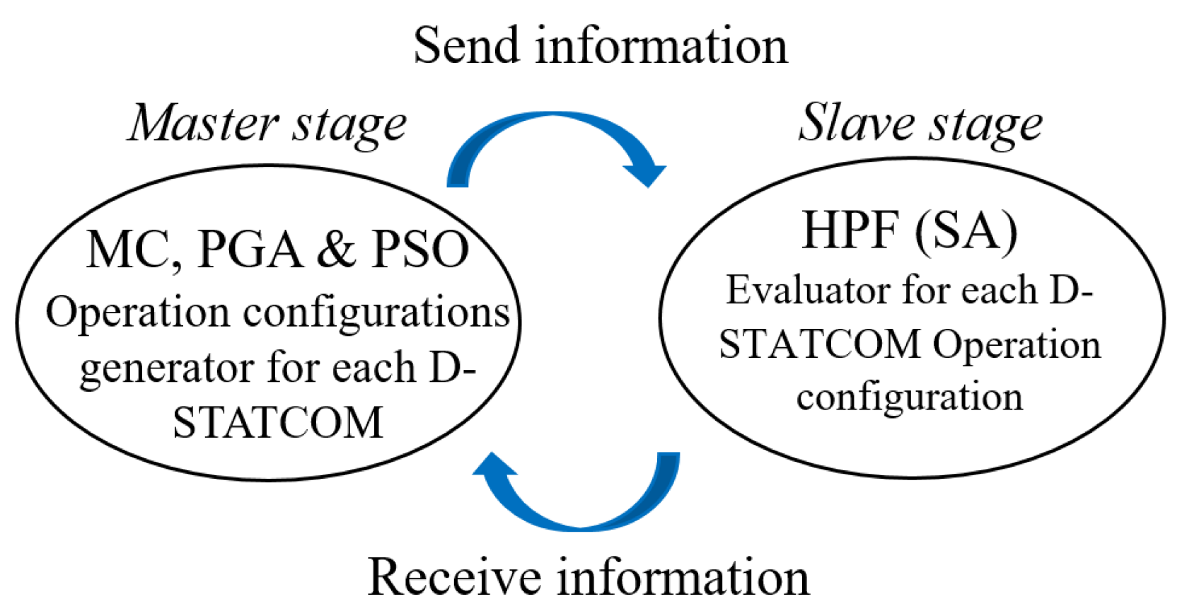
3. Proposed Methodology

In this section, we present the proposed master–slave solution methodology, which divides the problem-solving process into two stages, taking into account variations in power demand and reactive power injection by D-STATCOMs over different time periods. In the proposed methodology, the master stage solves the problem of smart operation of D-STATCOMs using three metaheuristic optimization techniques that work with continuous variables (as dictated by the nature of the reactive power dispatch problem under consideration). For its part, the slave stage evaluates the impact of each solution on the defined objective functions and constraints [37].

To facilitate the exploration of the optimization techniques in infeasible regions, expedite algorithm convergence, and avoid frequent entrapment in local optima [44], we employed a fitness function. This function penalizes the objective function if any of the model’s constraints are violated. For the sake of simplicity, this fitness function will be here referred to as the objective function and is presented in Equation (10).

$$FO=F{O}_n+\alpha Pe{n}_V+\beta Pe{n}_I$$

(10)

In this equation, $F{O}_n$ corresponds to the objective function under analysis (either the minimization of energy losses or the reduction in CO₂ emissions). $Pe{n}_V$ and $Pe{n}_I$ represent the parameters that aggregate all voltage and current violations resulting from the power dispatch configurations proposed by the optimization techniques. Dimensionless factors $\alpha$ and $\beta$ are used to normalize the fitness function so that it penalizes the objective function according to the severity of the voltage and load violations. In this study, these factors take a value of 1000, which was determined through trial and error in multiple runs of the proposed solution methodologies [44]. Importantly, the power limits set for the D-STATCOMs are enforced through the implementation of the objective function, while the active and reactive power balances are maintained through load flow calculations.

In summary, the proposed methodology can be illustrated as given in Figure 1, which shows that the master stage generates the operation configurations proposed by the MC method, the PGA, and the PSO. These configurations are then sent for evaluation in the slave stage to determine the impact of the proposed power configurations on the network and provide a value to the objective function by calculating the HPF based on successive approximations. Under this framework, the optimization techniques progress through their iterative processes with the aim of finding the highest-quality solutions.

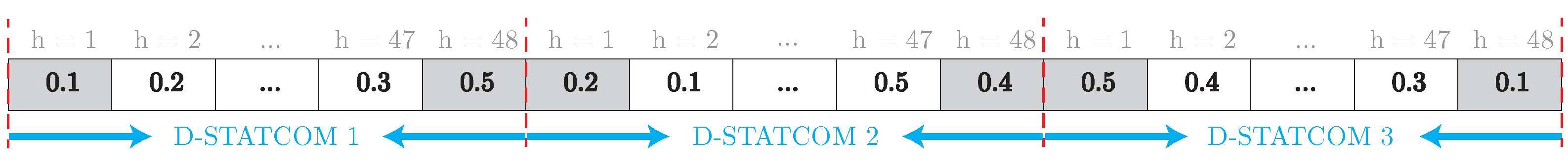
3.1. Proposed Encoding

For the proper execution of the proposed methodology, the master stage requires an encoding that can represent different solutions to the problem being addressed. Such encoding should consider problem-specific characteristics, such as constraints, variable type and quantity, or the peculiarities of each algorithm [45]. In this paper, the proposed encoding encompasses the power dispatch of the three D-STATCOMs installed in the network over different time periods.

There exist various ways to represent the encoding of an optimization problem, including binary, real-value, or permutation-based encoding schemes [45]. In this case, we employed an encoding consisting of continuous variables restricted to the operational range of the D-STATCOMs. The representation of each solution is depicted in Figure 2, where the encoding consists of a 1 × 144 vector. Each column in this vector represents the power to be injected by the three operational D-STATCOMs into the network at each time period. Given that power demand data are collected every 30 min, it means that a day’s operation is defined by 48 variables (1 × 48).

3.2. Master Stage

In the proposed methodology, the master stage hosts the optimization techniques responsible for generating the dynamic operation configurations for the D-STATCOMs [14]. In the specialized literature, various optimization techniques are available to address continuous nonlinear programming problems. These techniques can be categorized into five main groups: analytical methods, artificial neural network-based approaches, metaheuristics techniques, sensitivity-based methods, and combinations of metaheuristics and sensitivity analysis [15]. However, metaheuristic techniques are the most widely used methodologies for solving problems related to the optimal sizing, location, and operation of electrical equipment in electrical networks [15]. These techniques are characterized by their stochastic nature and are typically population-based, making them suitable for addressing problems involving continuous, discrete, or hybrid variables [15]. Among them, bio-inspired algorithms have shown to be the most effective and widely employed, with techniques based on the behavior of ant colonies [4], eagles [46], and birds [14], among others, standing out. For our research, the MC method, the PGA, and the PSO were identified as the most efficient strategies for power dispatch problems such as that discussed in [37]. We selected these algorithms to evaluate their performance in solving the problem of intelligent power dispatch of D-STATCOMs in power distribution systems.

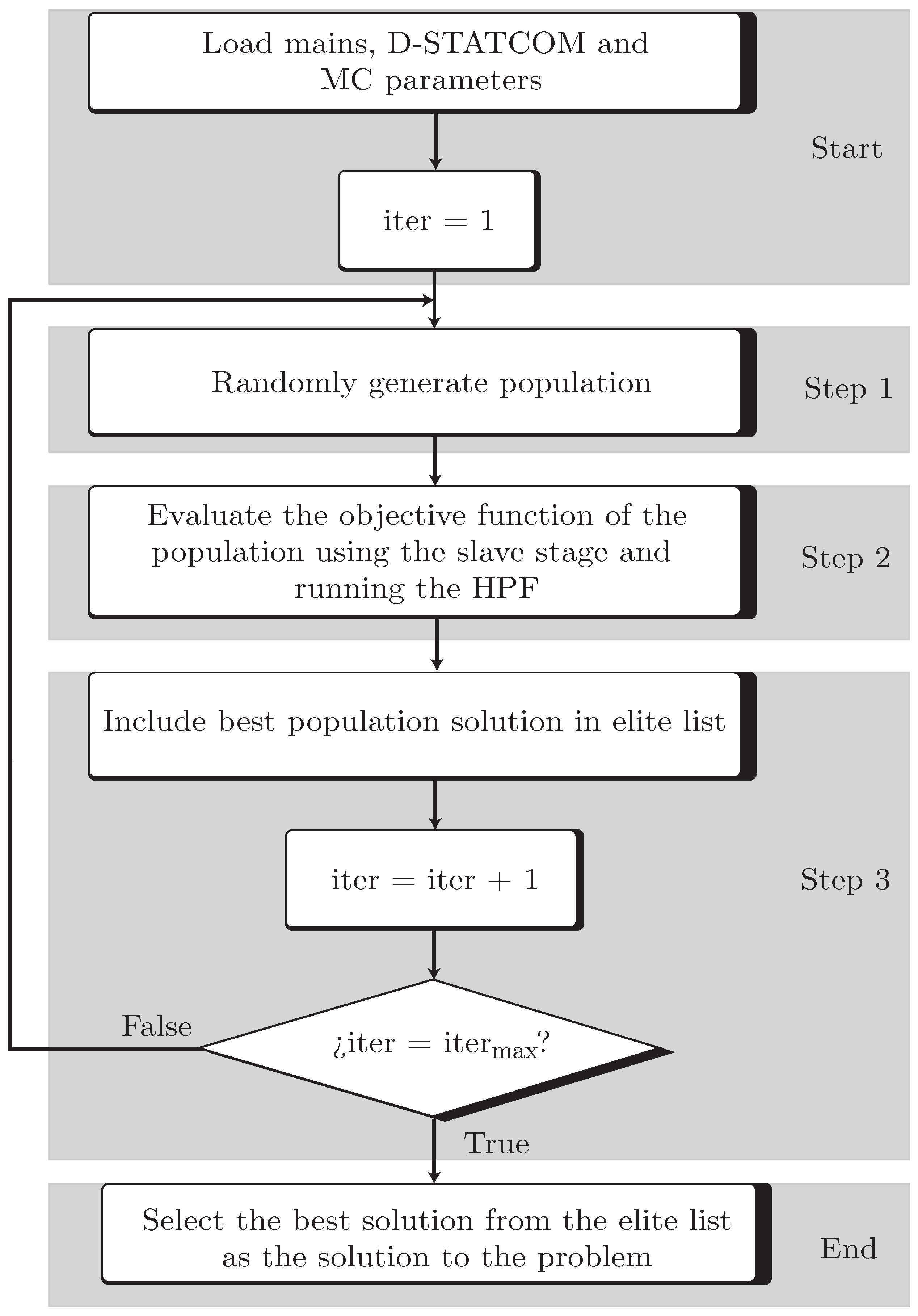
3.2.1. Monte Carlo Method

The Monte Carlo (MC) method entails a sequence of states whose evolution is governed by random events [47]. It operates by generating a population of random individuals in each iteration, with each representing a potential solution to a given problem. After evaluating the objective function of each individual and confirming that all constraints are satisfied, the individual with the best solution, also known as the incumbent, is included in an “elite list.” At the end of the iterative process, the best solution is selected from this list [37].

Adapting the MC method to the problem of intelligent power dispatch of D-STATCOMs involves considering the continuous encoding proposed in Figure 2 and fine-tuning the algorithm’s parameters as reported in Section 5.

Figure 3 shows the flowchart of the iterative process followed by the MC algorithm.

3.2.2. Population-Based Genetic Algorithm

The genetic algorithm (GA) stands as one of the most extensively researched evolutionary optimization techniques, primarily due to its remarkable performance and solution speed [48]. Classically, this optimization algorithm is built on five key principles, which are elaborated in [45] and summarized as follows:

• Population generation: This principle stems from the fact that, in nature, the probability of survival is greater within communities than in solitary individuals. Hence, the GA employs populations of individuals (generations) to converge.
• Selection: This principle originates from a natural law that limits reproduction to certain individuals in a population, allowing only the fittest members to have higher chances of having offspring. Under this principle, the algorithm ensures that subsequent generations will outperform their predecessors.
• Encoding: This principle is based on how the individual characteristics of each solution are encoded, which influences the algorithm’s efficiency and its search space. It also impacts the adaptation of individuals to the problem’s constraints.
• Crossover: This principle deals with how individuals from the initial generation are recombined to shape the genetic structure of the successor generation. It facilitates the mixing of specific traits from population members and is the basic mechanism of evolution.
• Mutation: This process reveals the random nature of generating individuals by modifying the characteristics already defined in their structures. It enables the exploration of solutions that might otherwise remain undiscovered.

Unlike the traditional GA, the adapted version used in this study to solve the problem of intelligent power dispatch of D-STATCOMs considers the continuous encoding proposed in Figure 2. In addition, the employed GA is population-based (PGA) [49]. Essentially, it adheres to the same principles as the GA, except that when updating generations, it no longer creates a single child to replace each parent. It can now be N children (mixed with the parents) that replace their preceding generation.

Figure 4 shows the flowchart of the iterative process followed by the PGA, and its tuned parameters are presented in Section 5.

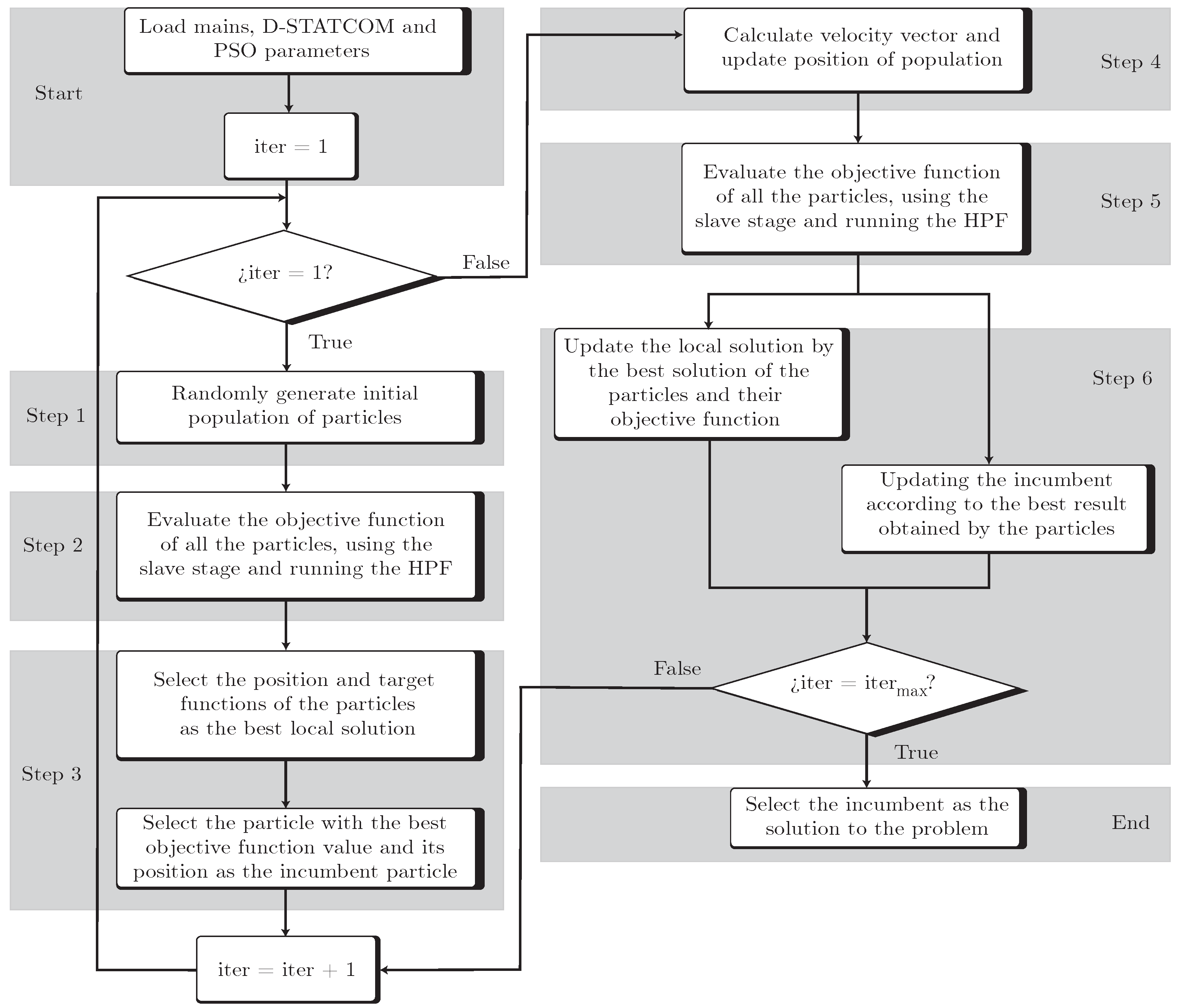
3.2.3. Particle Swarm Optimization

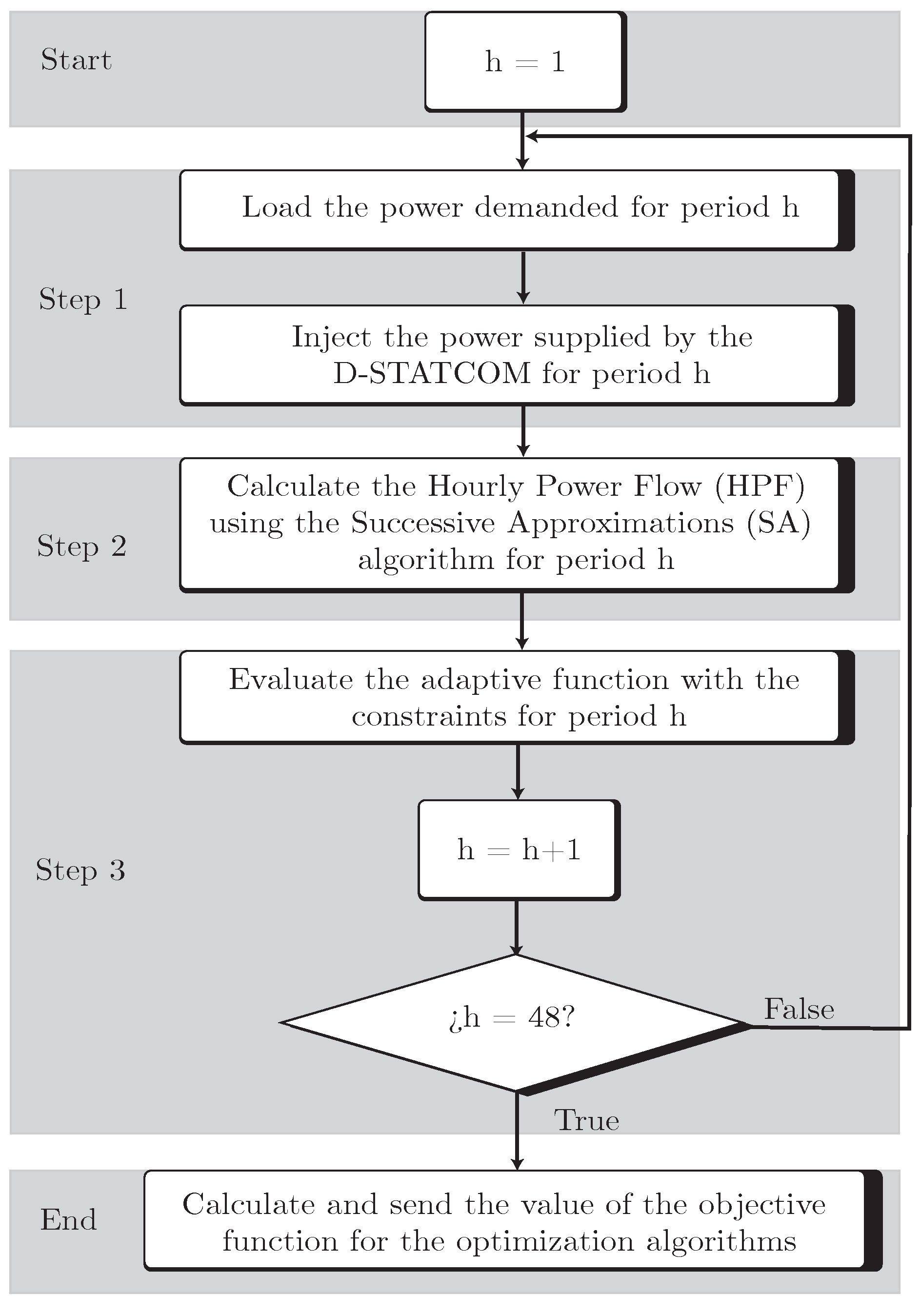
Particle Swarm Optimization (PSO) is a bio-inspired optimization technique that emulates the behavior of individuals within a swarm or cluster to maximize the survival of their species [50]. In this technique, each individual navigates through the solution space based on its individual experience and the collective experience of the group [51]. Its advantages lie in its efficiency, robustness in controlling variables, and straightforward concept [45].

Unlike the traditional PSO, the adapted version employed in this study to address the problem of intelligent power dispatch of D-STATCOMs considers the continuous encoding proposed in Figure 2.

Figure 5 illustrates the flowchart representing the iterative process of the PSO, and its tuned parameters are presented in Section 5.

3.3. Slave Stage

The slave stage constitutes the second part of the proposed methodology for solving the problem of intelligent operation of D-STATCOMs to minimize energy losses and CO₂ emissions (see Figure 1). This stage is responsible for determining the fitness function and feasibility of each potential solution proposed by the master stage [44]. In other words, the slave stage computes the electrical variables required to estimate the system’s energy losses and emissions while ensuring compliance with the set of constraints representing the problem. Figure 6 presents the flowchart of the iterative process followed by the slave stage, whose interpretation is detailed below.

• Start: Each solution is evaluated for a day of operation, which comprises 48 time periods (h). These periods represent the energy demand data collected every half hour. Moreover, Steps 1 to 3 are repeated until the last period is evaluated.
• Step 1: The initial parameters of the network (e.g., demanded power, future locations of the D-STATCOMs, and current limits) are loaded without considering the presence of D-STATCOMs. Then, the reactive power operation configurations obtained from the algorithms’ solutions are implemented in the system, which seek to have an impact on it either by reducing energy losses or CO₂ emissions.
• Step 2: The HPF is computed using the method of successive approximations—a numerical technique that involves finding the roots of an equation within a specified number of iterations [52]. This method calculates the voltage magnitudes in a network, which are later used to find the value of the objective functions and system’s constraints. The formulation employed for the method of successive approximations is as presented in Equations (11) and (12), following the formulation reported in [14].

  $${\mathbf{S}}_g^{\ast }=Diag\left({\mathbf{V}}_g^{\ast }\right)\left(Y_{gg}{\mathbf{V}}_g+Y_{gd}{\mathbf{V}}_d\right)$$

  (11)

  $$-{\mathbf{S}}_d^{\ast }=Diag\left({\mathbf{V}}_d^{\ast }\right)\left(Y_{dg}{\mathbf{V}}_g+Y_{dd}{\mathbf{V}}_d\right)$$

  (12)

  In these equations, ${\mathbf{S}}_g$ is the generated power, and ${\mathbf{S}}_d$ denotes the power demanded by the distribution system. Similarly, ${\mathbf{V}}_g$ and ${\mathbf{V}}_d$ represent the voltages at the generation and demand nodes, respectively. Furthermore, $Y_{gg}$, $Y_{dg}$, $Y_{gd}$, and $Y_{dd}$ are the components of the nodal admittance matrix, with each component relating the admittance data associated with slack bus to slack bus, demand bus to slack bus, generation bus to demand bus, and demand bus to demand bus, respectively. Finally, since ${\mathbf{V}}_d$ represents the variables of interest, the method of successive approximations iteratively solves Equation (13).

  $${\mathbf{V}}_d^{t+1}=-Y_{dd}^{-1}(Dia{g}^{-1}\left({{\mathbf{V}}_d}^{t,\ast }\right){\mathbf{S}}_d^{\ast }+Y_{dg}{\mathbf{V}}_g)$$

  (13)
• Step 3: The fitness function of Equation (10) is evaluated, which comprises the value of the original objective function (minimization of energy losses or reduction in CO₂ emissions) and the constraints added through penalties. In simpler terms, the aim is to develop an indicator that notifies the presence of infeasible solutions. This way, it is possible to identify solutions that appear to be of excellent quality in terms of reductions yet violate voltage and/or load constraints. The best-case scenario for the fitness function is when it equals the objective function (zero penalties).
• End: Once the value of the fitness function has been determined, it is passed to the slave stage to continue the process, and this is repeated for each solution.

4. Test Systems

To validate the proposed methodologies for the intelligent operation of D-STATCOMs in PDSs, we employed two test systems, as well as an adapted version of one of them to test the winning methodology in a system with the power demand characteristics of a feeder in the city of Talca in Chile. The two test systems correspond to the 33- and 69-node radial feeders reported in [20]. The adapted system, for its part, uses demand data from a feeder owned by Compañía General de Electricidad S.A. in Talca (Chile). For each test system, we present their parameters, electrical configurations, and demand curves employed for the HPF calculations in the slave stage of the proposed methodology.

The selection of the 33- and 69-node radial distribution systems as test scenarios in this study is not only justified by their extensive use in the specialized literature but also by their structural and operational characteristics, which closely resemble real-world medium-voltage feeders. These systems provide a well-balanced combination of modeling complexity and computational tractability, making them suitable for validating optimization-based methodologies. Furthermore, their topological simplicity facilitates the integration of real operating constraints and variable demand profiles, as demonstrated by the adaptation of the 33-node system to the conditions of the Vaccaro feeder in Chile (Section 4.3). Their widespread recognition also ensures benchmarking consistency and the reproducibility of results across related research efforts.

Table 1. General parameters of the test systems considered in this study.

Parameter	Value	Unit
$E{F}_i^g$	0.1643	${\displaystyle \frac{\mathrm{kg}{\mathrm{CO}}_2}{\mathrm{kWh}}}$
$\mathcal{H}$	24	h
$\mathcal{N}$	(33 or 69)	Dimensionless
$Q_{min,max}^{\mathrm{D-STATCOM}}$	(0–500)	kvar
$V_i^{min,max}$	±8	%
$V_{base}$	12.66	kV
$S_{base}$	1000	kVA
${\mathrm{\Delta }}_h$	0.5	h

reports the general parameters included in the mathematical formulation described in Section 2, the nominal electrical values, and their corresponding baseline values.

Note that the voltage limit is set at ±8% of the fixed nominal voltage, following the NTCSSD criterion, which considers a medium-voltage low-density PDS.

Another common aspect between the test systems under analysis is the behavior of the average demand curve. This curve, as shown in Figure 7, represents the average active and reactive power behavior over a day of operation in a Colombian PDS [14]. The parameters used to construct this curve are presented in

Table 2. Behavior of daily active and reactive power demand in a Colombian power distribution system [20].

${\Delta }_{\mathit{h}}$ [$\frac{1}{2}$ h]	P [p.u.]	Q [p.u.]	${\Delta }_{\mathit{h}}$ [$\frac{1}{2}$ h]	P [p.u.]	Q [p.u.]	${\Delta }_{\mathit{h}}$ [$\frac{1}{2}$ h]	P [p.u.]	Q [p.u.]
1	0.1700	0.1477	17	0.3100	0.2497	33	0.4500	0.4226
2	0.1400	0.1119	18	0.3400	0.3224	34	0.4500	0.3081
3	0.1100	0.0982	19	0.3600	0.3263	35	0.4500	0.2994
4	0.1100	0.0833	20	0.3900	0.3661	36	0.4500	0.3336
5	0.1100	0.0739	21	0.4200	0.3585	37	0.4300	0.3543
6	0.1000	0.0827	22	0.4300	0.3316	38	0.4200	0.3399
7	0.0900	0.0831	23	0.4500	0.4187	39	0.4600	0.4234
8	0.0900	0.0637	24	0.4600	0.3652	40	0.5000	0.4061
9	0.0900	0.0702	25	0.4700	0.3382	41	0.4900	0.3820
10	0.1000	0.0875	26	0.4700	0.3614	42	0.4700	0.3820
11	0.1100	0.0728	27	0.4500	0.3877	43	0.4500	0.3887
12	0.1300	0.1214	28	0.4200	0.3434	44	0.4200	0.2751
13	0.1400	0.1231	29	0.4300	0.3771	45	0.3800	0.3383
14	0.1700	0.1390	30	0.4500	0.4269	46	0.3400	0.2355
15	0.2000	0.1410	31	0.4500	0.4224	47	0.2900	0.2301
16	0.2500	0.1998	32	0.4500	0.3647	48	0.2500	0.1818

, which specifies, from left to right, the fraction of time in half-hour intervals (${\mathrm{\Delta }}_h$) for each time period h and the demand for active power (P) and reactive power (Q) in per unit (p.u.).

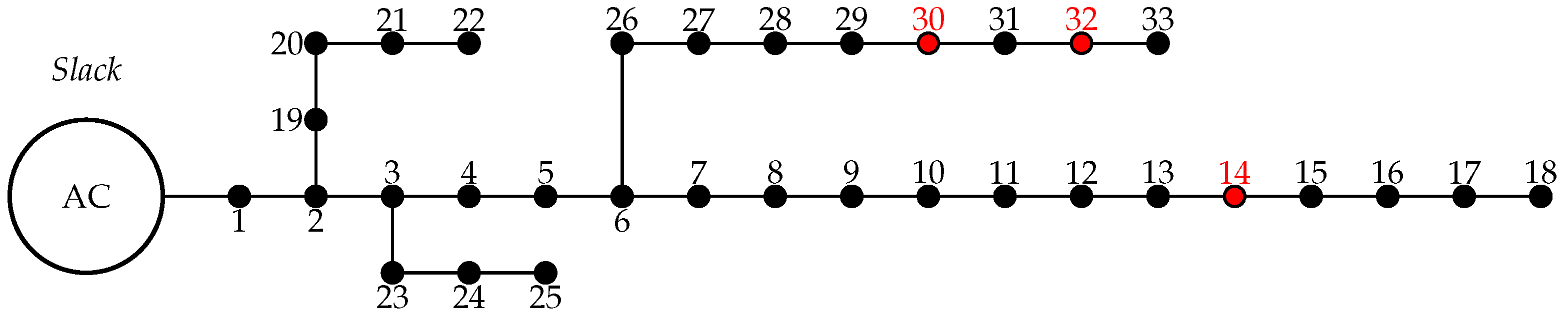
4.1. Thirty-Three-Node Radial Test System

Figure 8 illustrates the electrical configuration of the 33-node radial test system, which was employed to validate the optimization strategies considered in this study. This test system consists of 33 nodes, 32 lines, and an Alternating Current (AC) swing generator or slack generator connected to the first node. The nodes highlighted in red indicate the locations of the D-STATCOMs in the network. These locations were determined based on the results reported in [14] and the power injection ranges specified in Table 1.

Appendix A describes the electrical parameters of the 33-node test system. From left to right, it specifies the line number (l), the sending node (i), the receiving node (j), the resistance ($R_{ij}$) and the reactance ($X_{ij}$) of the line interconnecting nodes i and j, the nominal active power ($P_j$) and reactive power ($Q_j$) demanded at the receiving node, and the maximum current ($I_{ij}^{max}$) allowed for each line. Importantly, in this study, we treated the lines of the 33-node test system as telescopic lines, meaning that each line has a different current limit based on its proximity to the generator [14]. To calculate the maximum line currents, we conducted an HPF analysis in the 33-node test system without D-STATCOMs, considering the maximum power demand during the critical hour of the day (see Figure 7). After this calculation, we selected the conductors based on the current limits specified in RIC No. 4 [38].

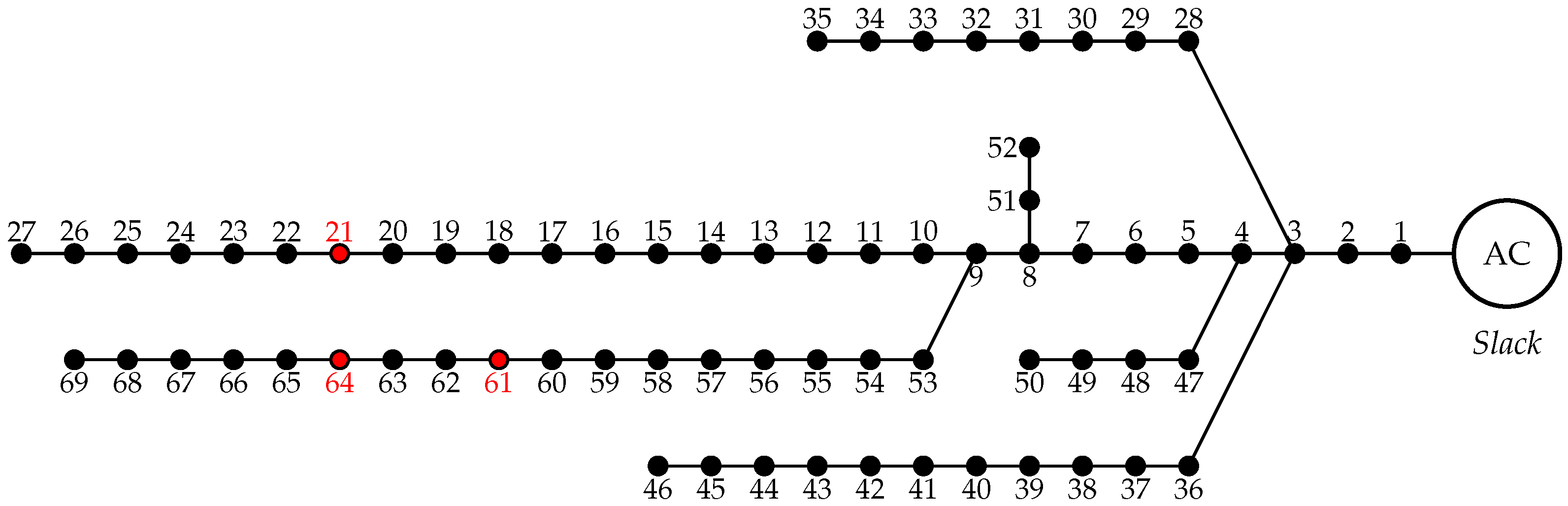
4.2. Sixty-Nine-Node Radial Test System

Figure 9 shows the electrical configuration of the 69-node radial test system, which was used to validate the optimization strategies considered in this study. This test system consists of 69 nodes, 68 lines, and an Alternating Current (AC) swing generator or slack generator connected to the first node. The nodes highlighted in red indicate the locations of the D-STATCOMs in the network. These locations were determined based on the results reported in [14] and the power injection ranges specified in Table 1.

The parameters of this test system are detailed in Appendix A, which is organized the same way as Appendix A.

4.3. Test System Adapted to the Characteristics of a Feeder in the City of Talca in Chile

In this study, we present a test system adapted to the characteristics of a feeder in the city of Talca in Chile, taking into account the following criteria:

• To select a test scenario, the literature suggests considering any reported system as a candidate for testing, as these systems have been created to replicate the behavior of real PDSs [14]. However, programmers must use their judgment to select the most appropriate one. In this case, the chosen candidate should represent the worst-case scenario in terms of voltage and/or load violations.
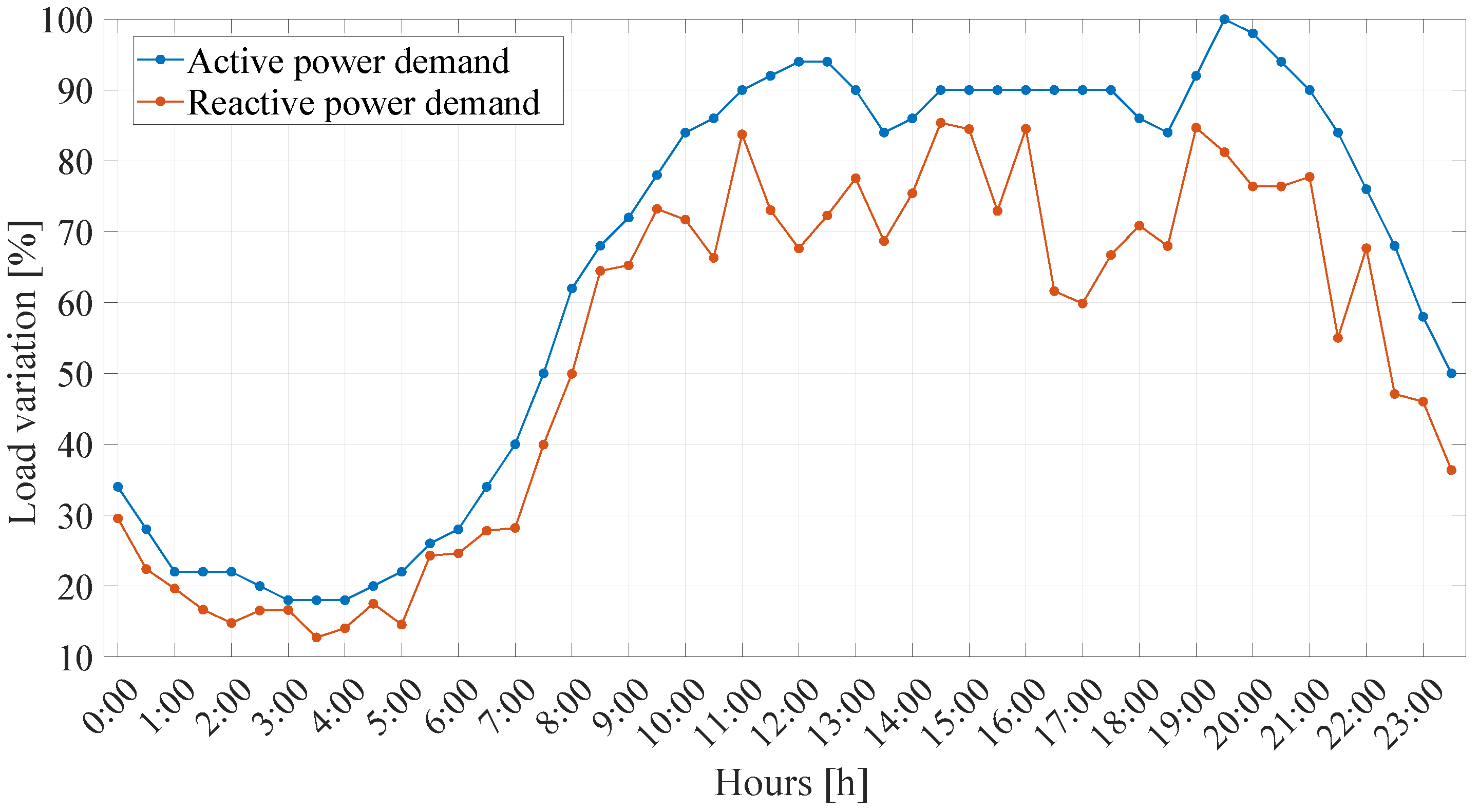
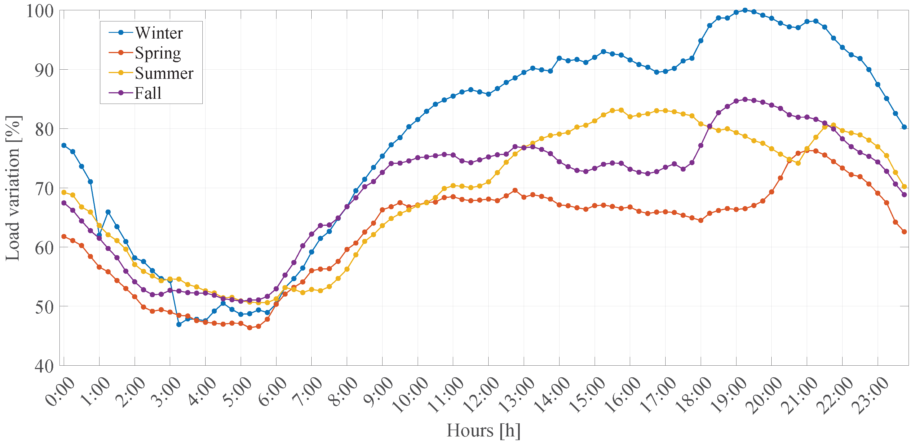
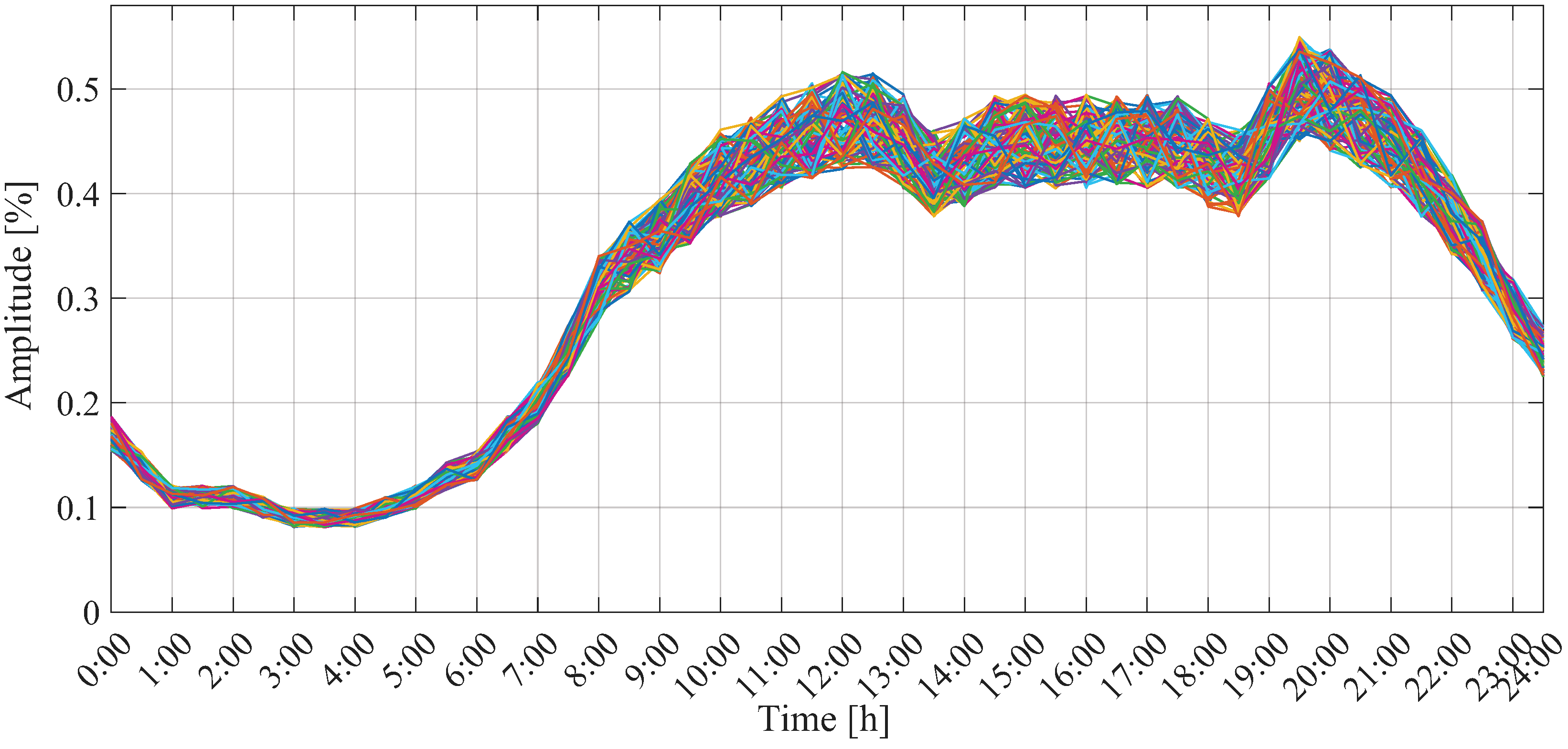
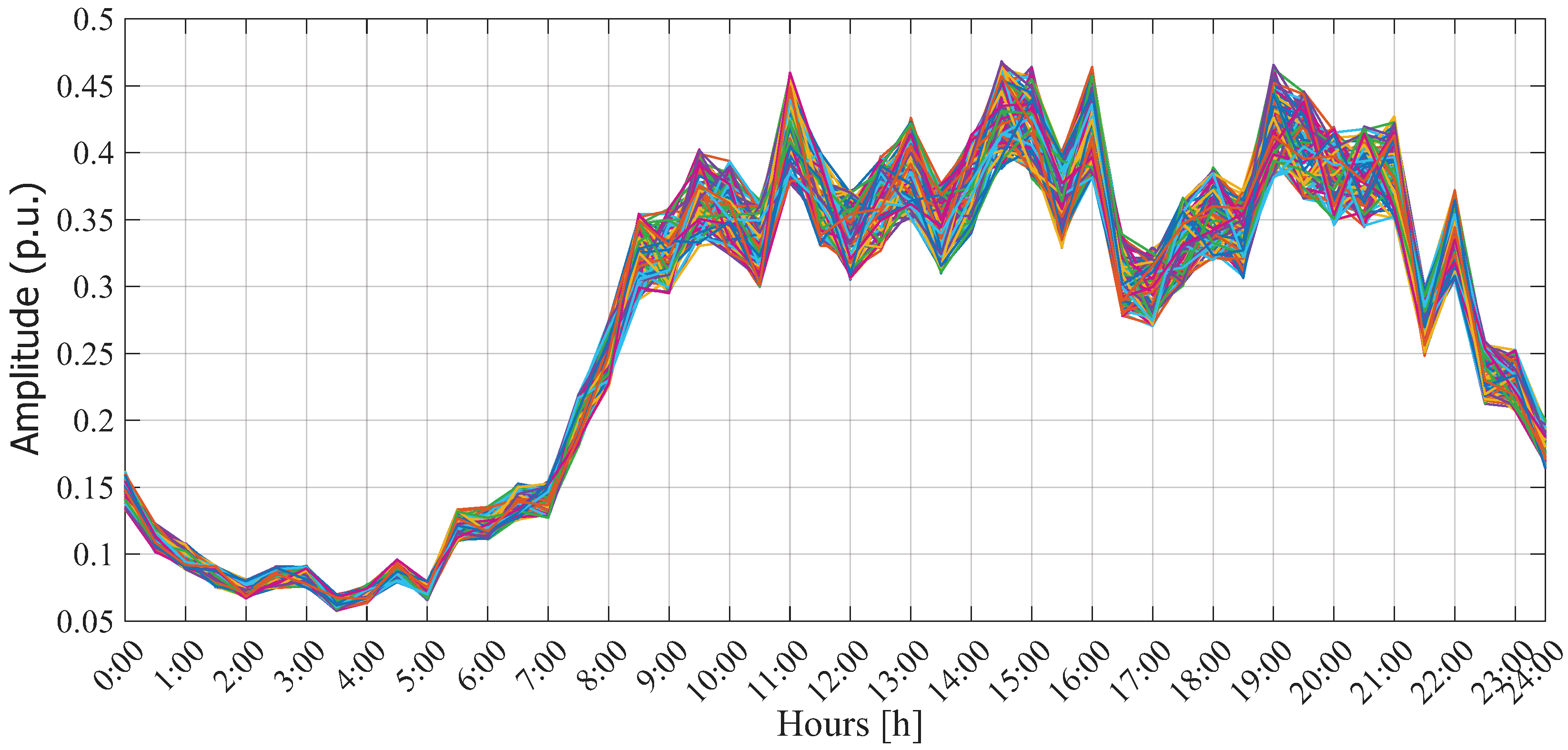
• According to Chilean regulations, the energy demand data of each feeder in Chile are available for access [53]. In this study, such data were used to replace the average demand curve of a Colombian PDS (see Figure 7). Although energy demand varies depending on the type of consumer (industrial, residential, or commercial), it is also influenced by the surrounding climatic conditions [54]. Hence, we here consider four different demand curves, one for each season (spring, summer, autumn, and winter).
• Since Talca’s feeder has four average demand curves, the current limit for each line must be recalculated by running an HPF that considers all four seasons. After this, we must select the highest currents throughout the year and follow the same procedure for conductor selection using RIC No. 4 [38].
• Another aspect worth mentioning regarding the demand curve is the time interval between measurements. In this adapted feeder, demand data are analyzed every 15 minutes, which modifies the encoding proposed in Section 3. In this case, a day of operation translates to 96 data points for each time period. Thus, the proposed encoding now includes a 1 × 288 vector, with each D-STATCOM injecting reactive power in a $1\times 96$ vector.
• The emission factor for conventional generators corresponds to that reported by the network operator in [55], i.e., 4.3278$e^{-1}\left[{\displaystyle \frac{\mathrm{Ton}{\mathrm{CO}}_2}{\mathrm{kWh}}}\right]$.

The Vaccaro feeder, located in the city of Talca in Chile and owned by Compañía General de Electricidad S.A., was selected as the candidate for testing due to its high power demand experienced between July 2022 and July 2023 [53]. The test system employed to model the Vaccaro feeder was the 33-node test system shown in Figure 8; hence, its parameters and baseline values are the same. The only difference lies in the determination of the current limits for the conductors, as an HPF must be conducted again considering the aforementioned factors.

Table 3. Updated current limits for the Vaccaro feeder.

Line	${\mathit{I}}_{\mathbf{ij}}^{max}$ [A]	Line	${\mathit{I}}_{\mathbf{ij}}^{max}$ [A]
1	410	17	99
2	307	18	99
3	266	19	99
4	195	20	99
5	195	21	99
6	195	22	99
7	99	23	99
8	99	24	99
9	99	25	114
10	99	26	99
11	99	27	99
12	99	28	99
13	99	29	99
14	99	30	99
15	99	31	99
16	99	32	99

presents the updated current limits for the Vaccaro feeder. Figure 10 and Figure 11, for their part, illustrate the weekly average active and reactive power demand for each season.

5. Simulation Results

The presentation of the results is divided into two parts. The first part discusses the fine-tuning of the optimization techniques used in the master stage, explaining their focus and the parameters employed to achieve the best results. The second part reports the results obtained by each technique in the different test systems under analysis.

To solve the problem of intelligent operation of D-STATCOMs in PDSs, all simulations were carried out using MATLAB^® 2022a on a Lenovo notebook with an Intel^® Core^TM i3 processor running at 2.1 GHz, 8 GB of RAM, and Windows 11, located at the Laboratory of Operation and Planning of Electrical Systems (LOPSE), operating in Curicó, Chile. Each simulation was executed 100 times to evaluate the performance of each methodology in terms of solution quality, average time, and standard deviation. To facilitate the numerical evaluation of all the optimization methods studied, the ${\mathrm{\Delta }}_h$ factor was set to $1\mathrm{h}$ for all simulation scenarios.

5.1. Fine-Tuning

Fine-tuning each optimization technique implemented in the master stage is one of the crucial steps in the proposed solution methodology [45]. Given the myriad options available, there is no specific way to accomplish this task. Therefore, the method used in this study to fine-tune each technique was based on a heuristic approach. It involves selecting the parameters that yield the best results, and these parameters vary depending on the test scenario and the objective function under consideration.

Table 4. Tuned parameters for the 33- and 69-node radial test systems.

Test Systems			33-Node Test System		69-Node Test System
Techniques	Parameters	Range	${\mathit{FO}}_{\mathbf{1}}$	${\mathit{FO}}_{\mathbf{2}}$	${\mathit{FO}}_{\mathbf{1}}$	${\mathit{FO}}_{\mathbf{2}}$
MC method	Number of individuals	[50–2000]	500	500	500	1000
	Number of iterations	[100–2000]	1000	1000	1000	1000
PGA	Number of individuals	[50–300]	300	300	300	300
	Number of iterations	[300–6000]	6000	2500	2500	2500
	Number of mutations	[5–20]	5	5	5	5
PSO	Number of individuals	[50–2000]	2000	2000	2000	500
	Number of iterations	[200–1500]	500	500	500	200
	Maximum inertia	[0.2–1]	0.8	0.5	0.8	0.8
	Minimum inertia	[0–0.6]	0.6	0.2	0.6	0.6
	Cognitive factor	[0.5–2]	2	0.5	2	2
	Social factor	[0–2]	1	2	1	1
	Velocity vector limit	[0.05–0.5]	0.05	0.05	0.05	0.05

shows the parameters selected during the implementation of each solution methodology in the 33- and 69-node test systems. From left to right, it specifies the optimization technique that was implemented, the parameters that were tuned in each technique, and the tuned values obtained for the different objective functions in each test system. Since the techniques differ in the number of parameters they possess, performing the same fine-tuning on each technique is challenging.

5.2. Results Obtained in the 33- and 69-Node Test Systems

In this subsection, we analyze the results of applying the proposed master–slave methodology to solve the problem of intelligent operation of D-STATCOMs in PDSs, with a specific focus on reducing energy losses and CO₂ emissions. Our analytical approach involves assessing each test system, beginning with a comprehensive statistical analysis of the results, followed by a more detailed graphical analysis.

5.2.1. Statistical Analysis

Table 5. Results obtained by each proposed master–slave methodology for each objective function and test system.

Test Systems		33-Node Test System		69-Node Test System
FOn		FO1 [kWh]	FO2 [TonCO2]	FO1 [kWh]	FO2 [TonCO2]
Base case		4444.3038	19.7346	4719.2523	20.6785
Solution reported in the literature [14]		3568.6463	19.5907	3729.9182	20.5159
Average reduction
Method	MC method	3522.6095	19.5831	3700.8778	20.5103
	PGA	3348.9625	19.5548	3488.3604	20.4762
	PSO	3349.9758	19.5553	3488.5301	20.4771
Maximum reduction
Method	MC method	3506.41	19.5798	3680.827	20.5069
	PGA	3348.6279	19.5548	3487.7505	20.4761
	PSO	3345.8634	19.5547	3482.3152	20.4757
Average standard deviation [%]
Method	MC method	0.1735	0.0054	0.2297	0.0054
	PGA	0.0035	0.0001	0.0068	0.0001
	PSO	0.0792	0.0015	0.1018	0.0039
Average processing time [s]
Method	MC method	1929.2804	1867.3774	4893.1803	11,204.963
	PGA	6356.2218	3523.6951	7632.2218	8241.9134
	PSO	3945.1104	3400.9324	8242.0869	990.3428
Accuracy [%]
Method	MC method	0.4598	0.0168	0.5417	0.0166
	PGA	0.0099	0.0003	0.0174	0.0003
	PSO	0.1227	0.0031	0.1781	0.0071

presents the results derived from testing the three proposed optimization methodologies to address the problem of intelligent operation of D-STATCOMs in PDSs. Particularly, it specifies the results obtained by each in the 33- and 69-node radial test systems in terms of minimum and average solution, average processing times, average standard deviation, and accuracy (which indicates how far the best solution is from the average solution) for the two objective functions guiding the optimization process: minimization of energy losses ($F{O}_1$) and reduction in CO₂ emissions ($F{O}_2$). Also, it presents the base cases for each test system, i.e., the energy losses and CO₂ emissions prior to considering the presence of D-STATCOMs in the network. Additionally, it includes the solutions proposed by the authors of [14], who suggested reducing energy losses via fixed reactive power injection. These solutions were taken into consideration for comparison purposes because these authors’ proposed strategy for the optimal integration and operation of D-STATCOMs in electrical networks yielded numerically sound results. Moreover, we must stress how important it is to create variable reactive power operation scenarios, as performed in the aforementioned study.

From the information presented in Table 5, we may highlight the following results:

• When analyzing the performance of the algorithms after being executed 100 times, the PGA exhibited the best repeatability over time and obtained the lowest average reduction in both test systems and both objective functions. Regardless of processing time or the number of times the technique was run, it consistently outperformed the others. For the 33-node test system, it achieved an average reduction of 24.646% in energy losses and 0.9109% in CO₂ emissions. In the case of the 69-node test system, it obtained an average reduction of 26.0823% in energy losses and 0.9784% in CO₂ emissions.
• Regarding average standard deviation, the PGA was the best-performing technique, with an average value of 0.0026% in both test systems and both objective functions. Although it did not yield the best minimum solution in any case, it proved to be the most reliable strategy due to its minimum solution being very close to the average solution in all simulation scenarios, with an average accuracy of 0.0069% with respect to the best solution. This demonstrates the PGA’s superior performance in terms of repeatability, as its very small standard deviation ensures consistent results every time it is executed.
• Despite the PGA being the best technique in terms of solution quality, one of its major drawbacks was its average processing time. According to the results, it required an average processing time of 6438.5130 seconds in both test systems and for both objective functions. Importantly, since the problem under analysis involves dispatching power for an entire day, the PGA’s average processing time (1.78 h) is reasonable in the context of the 24-hour time horizon under analysis. This allows network operators to explore multiple scenarios in short processing times.
• The other methodologies also yielded positive results, occasionally outperforming the PGA. For instance, the PSO consistently provided the best solution in each study case. Notably, in the case of energy losses in the 69-node test system, it achieved reductions of 26.2104%. It also demonstrated a remarkable performance in terms of computational speed and the ability to find minimum solutions. It, however, showed a tendency to converge to local optima as the number of individuals and iterations increased, whereas the PGA maintained its effectiveness. The MC method, for its part, provided better solutions than those proposed in [14]—a study serving as a reference for this research. Still, due to its inherent stochastic nature, it did not consistently deliver high-quality solutions with repeatability over time. For the MC method, expanding the exploration space increases the likelihood of obtaining high-quality solutions but also extends processing times, as observed in the 69-node test system regarding reduction in CO₂ emissions, where its average processing time exceeded three hours.

Table 6. Performance of the PGA in comparison to the other algorithms.

Test Systems		33-Node Test System		69-Node Test System
${\mathit{FO}}_{\mathit{n}}$		${\mathit{FO}}_{\mathbf{1}}$	${\mathit{FO}}_{\mathbf{2}}$	${\mathit{FO}}_{\mathbf{1}}$	${\mathit{FO}}_{\mathbf{2}}$
Average reduction [%]
Method	MC method	4.9294	0.1444	5.7423	0.1661
	PSO	0.0302	0.0026	0.0048	0.0044
Maximum reduction [%]
Method	MC method	4.4998	0.128	5.2454	0.1498
	PSO	−1.0826	−1.0001	−1.156	−1.0023

reports the performance of the PGA when compared to the other optimization techniques (considering both objective functions and both test systems). As observed, the PGA outperformed the PSO and the MC method in terms of average solutions. The most significant difference was observed in the 69-node test system, where the PGA outperformed the MC method by 5.7423% in terms of reduction in energy losses. The PSO, for its part, was the best-performing method concerning minimum solutions (the negative sign indicates that the PGA was outperformed). This was most noticeable in the 69-node test system (also when analyzing energy losses), where the PSO outperformed the PGA by 0.156%. Moreover, the PGA’s performance in reducing CO₂ emissions was also superior to that of the MC method and the PSO.

5.2.2. Graphical Analysis

In this subsection, we delve deeper into the results, examining the reductions achieved by each algorithm and the operational impact of the solution provided by the PGA on each test system under analysis.

• Thirty-Three-Node Test System

Figure 12 illustrate the maximum and average reductions (in percentage) obtained by each algorithm for both objective functions when compared to the base case and the solution proposed in the literature for the 33-node test system. In general, all methods proved to be superior to the base case and outperformed the constant reactive power injection solution proposed in [14]. This latter, as reported in [14], was able to reduce energy losses by 19.7029% and CO₂ emissions by 0.7293% compared to the base case.

Particularly in terms of CO₂ emission reductions, there was not a significant difference in both cases (average and maximum reductions) when compared to the base case. This is because reactive power injection does not directly correlate with emission reduction. Emissions primarily depend on the active power supplied by the generator. That said, the most notable impact of intelligent reactive power injection was observed in the reduction in energy losses, which are directly influenced by improved voltage profiles.

Concerning energy losses, the average reductions achieved by each algorithm when compared to the base case (see Figure 12) were above 20%. Regarding CO₂ emissions, the average reductions were all above 0.7676% (solution obtained by the MC method). From Figure 12, it is clear that the PSO obtained the maximum reduction in energy losses and CO₂ emissions, with values of 24.7157% and 0.9115%, respectively. However, the PGA yielded the best average reductions, with a value of 24.6460% for energy losses and 0.9109% for CO₂ emissions. Based on these results, we may conclude that, considering a year of operation, the PGA is capable of reducing energy losses by 399.7995 MWh and CO₂ emissions by 65.627 $Ton{\mathrm{CO}}_2$.

Moreover, when comparing the average reductions obtained by each algorithm to the constant reactive power injection solution reported in the specialized literature (see Figure 13), it is evident that the latter does not make the most of the existing distributed energy resources installed in the network. For instance, when analyzing the performance of the best strategy (PGA), it achieved higher average reductions in energy losses and CO₂ emissions, with values of 6.1559% and 0.1829%, respectively. Considering a year of operation, these indicators equate to reducing energy losses by 80.1845 MWh and CO₂ emissions by 13.1035 $Ton{\mathrm{CO}}_2$, meaning that the PGA produces better results than the constant reactive power injection solution. This underscores the importance of flexible reactive power injection by the D-STATCOMs at the different operating hours within the time horizon under analysis. Similarly, the PSO was the method that achieved the highest reduction in energy losses and CO₂ emissions, outperforming the constant injection solution by 6.2428% in terms of energy losses and 0.1835% in terms of CO₂ emissions.

The intelligent injection of reactive power into PDSs has also been found to affect their operating characteristics, directly impacting nodal voltages and line loadability. Figure 14 shows the hourly behavior of the node with the lowest voltage (node 18) when we implemented the constant reactive power injection solution proposed in [14] and the dynamic solution provided by the PGA. From this figure, it is clear that allowing flexible reactive power injection improves the system’s nodal voltages, reducing the chances of being penalized by the local regulator due to voltage violations (in case of exceeding the $\pm 8\%$ limit of the nominal voltage). This is possible because dynamic reactive power injection adapts to the system’s demand conditions, allowing network operators to have a flexible response to any transient changes in reactive power demand.

Furthermore, as observed in Figure 14, no voltage levels exceeded the nominal value during the entire time horizon under analysis, indicating no overvoltage issues. Similarly, no undervoltage issues were observed from 00:00 to 10:30. However, between 11:00 and 21:00, voltage dropped to critical levels, reaching its lowest point at around 19:30. In this regard, both solutions (constant and dynamic reactive power injection) managed to effectively control these voltage drops. Nonetheless, the PGA’s intelligent solution led to a 2.6388% increase in nodal voltage (from 0.9095 to 0.9335 p.u.), whereas the constant injection solution only led to a 1.3633% increase in nodal voltage (from 0.9095 to 0.9219 p.u.). In the remaining hours following 21:30, nodal voltage returned to its initial behavior.

The dynamic injection of reactive power has a noticeable impact on voltage levels, which, in turn, affects the loadability of all the system’s lines. If we focus on analyzing the line with the highest load index (the most critical or overloaded) and ensure that it does not exceed 100%, we can be sure that the other lines of the system will experience the same effect. Figure 15 illustrates the performance of the most critical line in the 33-node test system (line 6) before and after implementing the intelligent strategy for D-STATCOM operation. As can be seen, between 00:00 to 07:00, the line exhibits the lowest loadability (below 40%). Hence, we observed no significant difference between the proposed strategies in terms of reducing this index during this time frame. However, from 07:30 to 18:30, the line’s loadability increased and fluctuated between 80% and 90%. Both injection strategies, thus, started to take effect, successfully maintaining the load below 90%. The most notable difference, nonetheless, was observed during the critical hour (i.e., at 19:30). Without any proposed strategy (without D-STATCOMs), the line’s loadability at this hour reached 99.2085%. Here, the proposed intelligent strategy excelled, reducing the load by 8.0127%, in contrast to a mere 5.0395% reduction achieved by the constant reactive power injection solution. At the end of the day, load levels dropped from 21:00 to 00:00, bringing the line’s loadability back to around 40%.

Based on the results of this analysis, along with those of the voltage profile assessment, intelligent power management using the PGA managed to lower energy losses and CO₂ emissions while enhancing the network’s technical aspects such as voltage profiles and line loadability. In light of this, the PGA is the best option for solving the problem under analysis in the 33-node test system.

• Sixty-Nine-Node Test System

In the case of the 69-node test system, Figure 16 and Figure 17 illustrate the maximum and average reductions (in percentage) achieved by each algorithm for both objective functions with respect to the base case and the solution proposed in [14]. This latter, as reported in [14], was able to reduce energy losses by 20.9637% and CO₂ emissions by 0.7863% compared to the base case. As in the 33-node test system, the results exhibited a consistent trend, featuring improvements in reductions compared to both the base case and the solution proposed in the literature, along with a significant impact on the network’s technical and operating conditions.

Interestingly, in most cases, larger reductions were recorded in the 69-node test system compared to the 33-node test system. For instance, as observed in Figure 16, which compares the reductions obtained by the methodologies with respect to the base case, the PSO achieved the highest reductions (best solution), with a 26.2104% reduction in energy losses and a 0.9811% reduction in CO₂ emissions. However, this methodology exhibited poor results in terms of repeatability compared to the PGA. In this case, the average reductions in energy losses and CO₂ emissions achieved by the PGA were 26.0823% and 0.9784%, respectively. Therefore, considering a year of operation, this translates to a reduction of 449.2755 MWh in energy losses and 73.8395 $Ton{\mathrm{CO}}_2$ in emissions.

When comparing the average reductions obtained by each algorithm to those of the constant reactive power injection solution proposed in the literature (see Figure 17), a similar pattern is observed as in the 33-node test system. Once again, the constant injection solution does not make the most of the distributed energy resources installed in the network. Comparatively, the dynamic solution provided by the PGA outperformed the constant injection solution, with average reductions of 6.4762% in energy losses and 0.1935% in CO₂ emissions. If we consider a year of operation, this equates to reductions of 88.1685 MWh in energy losses and 14.4905 $Ton{\mathrm{CO}}_2$ in emissions when compared to the constant injection solution. These results highlight the importance of allowing flexible power injection by the D-STATCOMs during the different operating hours within the time horizon under analysis.

Another notable aspect in Figure 17 is the performance of the MC method, which deviates from the trend of achieving larger reductions than in the 33-node test system. In this case, this method outperformed the solution proposed in the literature by only 0.7786% in average energy loss reductions and 0.0275% in average CO₂ emissions reductions. To some extent, this performance decline can be attributed to the stochastic nature of the MC method, which tends to get trapped in local optima as the solution space expands. In this test system, we also observed that the PSO provided the best solution. However, in terms of average solution and standard deviation, the PGA outperformed the PSO.

Furthermore, the 69-node test system exhibited a behavior similar to that of the 33-node test system regarding nodal voltages and line loadability, both of which were improved compared to the base case and the solution reported in the literature. Figure 18 shows the hourly behavior of the node with the lowest voltage (node 65) when we implemented the constant reactive power injection solution reported in [14] and the PGA’s dynamic solution. As can be seen, no voltage levels exceeded the nominal value, indicating no overvoltage issues. Similarly, no undervoltage issues were observed from 00:00 to 18:30, highlighting the excellent conditions of the system. Between 19:00 and 21:00, nonetheless, voltage dropped to critical levels, reaching its lowest point at around 19:30. In this regard, both solutions (constant and dynamic reactive injection) managed to successfully control these voltage drops. The intelligent solution provided by the PGA managed to increase nodal voltage by 1.8936% (from 0.9136 to 0.9309 p.u.), whereas the constant injection solution led to a 1.1164% increase in nodal voltage (from 0.9136 to 0.9238 p.u.). In the remaining hours following 21:00, nodal voltage returned to its initial behavior.

For the 69-node test system, we also analyzed the line with the highest load index (the most critical or overloaded). Figure 19 depicts the behavior of the most critical line (line 4) before and after implementing the intelligent strategy for D-STATCOM operation. As observed, from 00:00 to 07:00, the line exhibited the lowest loadability (below 40%). Hence, the proposed strategies did not significantly differ from each other in reducing this index. However, between 07:30 and 18:30, the line’s loadability increased to levels ranging between 80% and 90%. Here, both solutions started to take effect, maintaining the load below 82%. During the system’s most critical hour (i.e., at 19:30), the line’s loadability without any proposed strategy (without D-STATCOMs) reached 97.9329%. At this point, the performance of the proposed strategies began to differ: the constant reactive power injection reduced the load by 9.2902%, while the intelligent strategy reduced it by 13.3698%. At the end of the day, the load levels dropped from 21:00 to 00:00, bringing the line’s loadability back to around 40%.

Based on the results obtained in the 33- and 69-node test systems, the PGA consistently yielded the best average solutions with the lowest standard deviations, which ensures high-quality solutions every time it is executed. Moreover, the processing times required by this methodology were relatively short (two hours for an entire day of operation), enabling network operators to analyze multiple scenarios while ensuring the best solution quality for each period of operation.

5.3. Uncertainty Analysis

To further validate the robustness of the proposed optimization methodology under realistic operating variability, an uncertainty analysis was conducted based on the evaluation of 100 different daily demand profiles for both active and reactive power. These profiles were generated to simulate variations in consumer behavior and network conditions across a typical day and are illustrated in Figure 20 and Figure 21. Each curve represents a possible operating scenario within the uncertainty space, with different colors indicating distinct active and reactive power demand patterns.

In this analysis, only the PGA, identified in Section 5.2.1 as the most effective metaheuristic, was applied. For each of the 100 demand scenarios, a single execution of the PGA was performed. This approach avoids repeated runs per scenario since the statistical performance of the algorithm was already thoroughly analyzed in Section 5.2.1. The objective was to evaluate whether the quality of the solution obtained under the average daily profile could be maintained across a wide range of variable conditions.

The results, summarized in

Table 7. Statistical analysis of solution robustness under demand uncertainty using PGA.

System	Objective Function	Avg. Reduction	Relative Reduction [%]	STD (Absolute)	STD [%]
33-node	Power losses [kWh]	3349.7227	24.9246	63.8036	1.9047
	CO2 emissions [ton]	19.5162	0.9279	0.1550	0.7940
69-node	Power losses [kWh]	3488.5267	26.3816	67.9297	1.9472
	CO2 emissions [ton]	20.6414	0.9956	0.1624	0.7869

, demonstrate that the proposed methodology maintains a consistent level of effectiveness under uncertainty.

In both the 33-node and 69-node systems, the PGA consistently achieved high reductions in power losses and CO₂ emissions across all 100 demand scenarios. Notably, the average reductions obtained—3349.7227 kWh and 19.5162 ton CO₂ for the 33-node system, and 3488.5267 kWh and 20.6414 ton CO₂ for the 69-node system—are remarkably close to the maximum reductions achieved under the average daily demand profile presented in Table 5 (3348.6279 kWh and 19.5548 ton CO₂ for the 33-node system, and 3487.7505 kWh and 20.4761 ton CO₂ for the 69-node system).

Moreover, the relative reductions achieved by PGA were 24.9246% and 26.3816% for power losses in the 33- and 69-node systems, respectively, while the emission reductions reached 0.9279% and 0.9956%. These values are accompanied by very low standard deviations, with STD values below 2% in all cases (1.9047% and 1.9472% for power losses; 0.7940% and 0.7869% for emissions in both systems), highlighting the high consistency and repeatability of the optimization strategy.

This level of performance, even under significant demand variability, confirms that the proposed methodology maintains excellent solution quality and robustness. The results validate that the optimization strategy not only performs well under ideal or average conditions but also retains its effectiveness across a wide range of realistic operational scenarios.

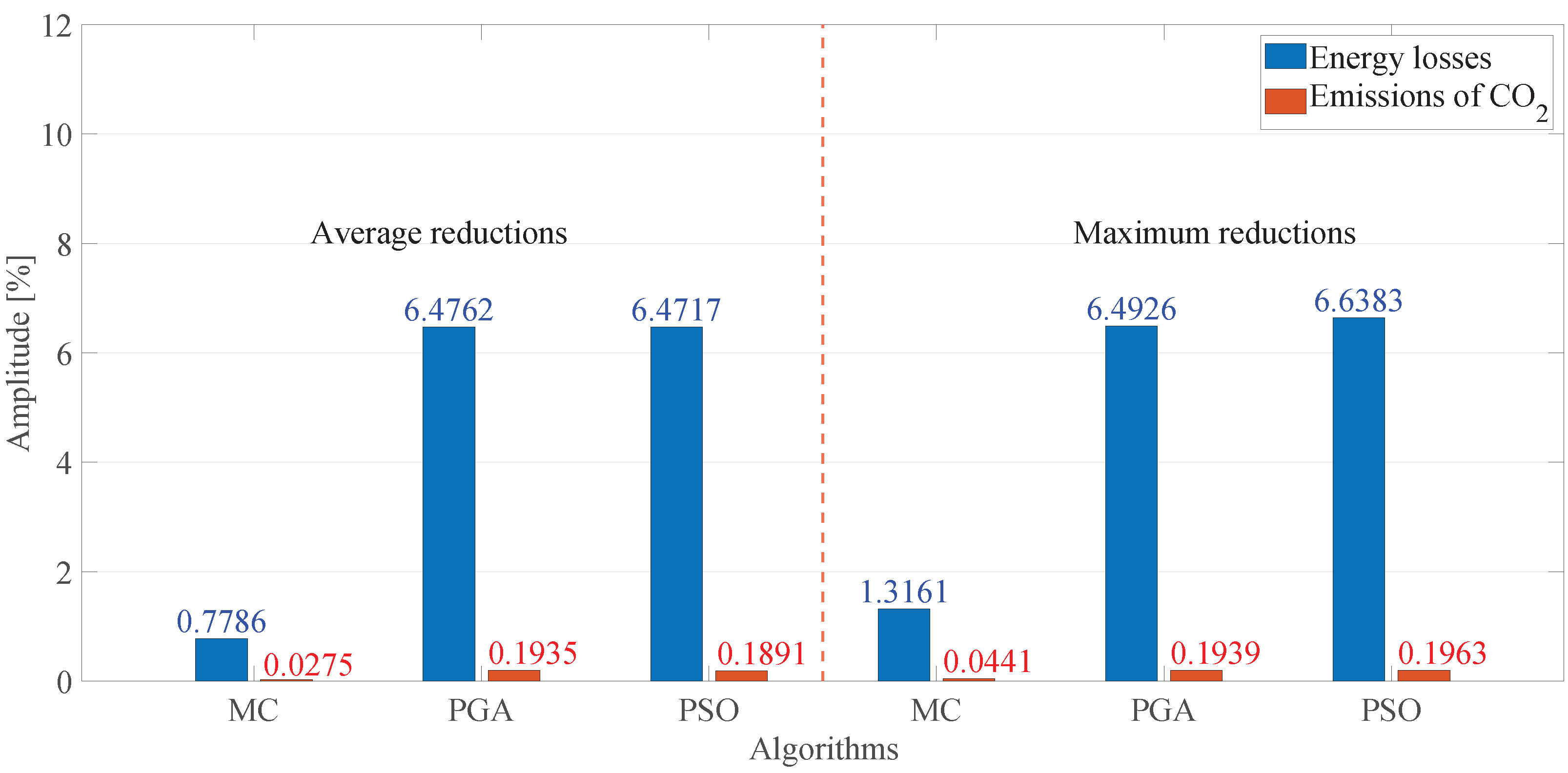
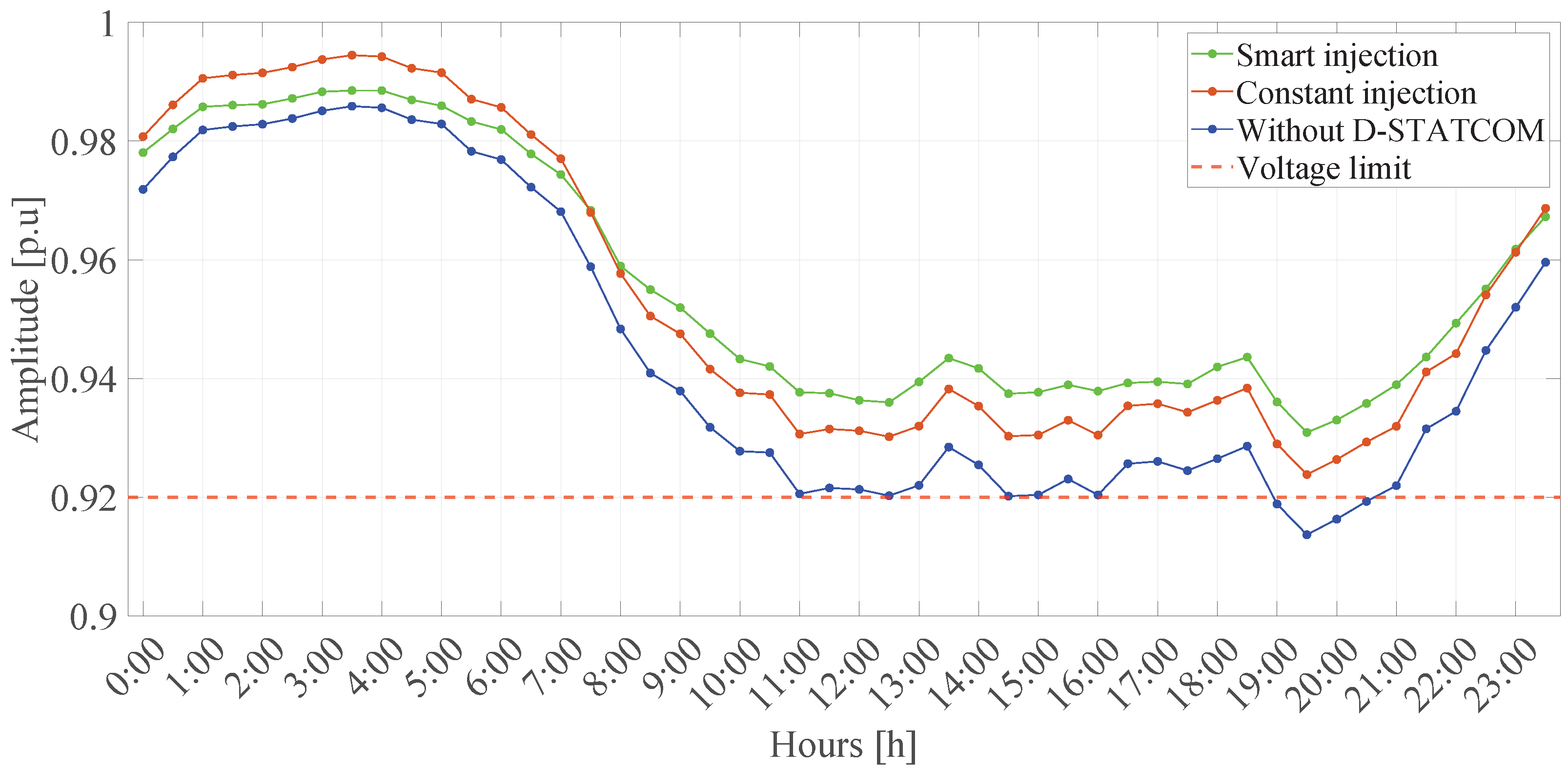
5.4. Results Obtained in the Vaccaro Feeder

In Section 3, we described a feeder that reflects the operating conditions of a distribution system located in the city of Talca in Chile. Notably, this feeder considers four study scenarios, corresponding to winter, spring, summer, and autumn from June 2022 to June 2023. In this subsection, we present a statistical analysis of the main results achieved after implementing the PGA in the aforementioned system. Additionally, we provide a detailed graphical analysis of the solutions produced by the proposed methodology in a test system adapted to the characteristics of a real distribution system owned by Compañía General de Electricidad in Chile.

5.4.1. Statistical Analysis

Table 8. Reductions achieved in the Vaccaro feeder after installing the D-STATCOMs.

${\mathit{FO}}_{\mathit{n}}$	${\mathit{FO}}_1$ [MWh]	${\mathit{FO}}_2$ [TonCO2]
Winter
Without D-STATCOMs	9.4738	12.5332
With D-STATCOMs	8.3872	12.4862
Processing time [s]	13,919.2009	5818.3968
Spring
Without D-STATCOMs	6.7983	9.9561
With D-STATCOMs	5.169	9.8857
Processing time [s]	9287.817	4012.5191
Summer
Without D-STATCOM	9.7885	11.0652
With D-STATCOMs	6.5103	10.9235
Processing time [s]	10,090.7899	3847.156
Autumn
Without D-STATCOM	8.3045	11.095
With D-STATCOM	6.4402	11.0144
Processing time [s]	12,255.1628	4952.9754

reports the impact of integrating D-STATCOMs into the selected distribution system (Vaccaro feeder). Particularly, it shows the values of each objective function under analysis before and after considering the intelligent operation of D-STATCOMs during the different seasons of the year, along with the processing times required by the PGA. Importantly, standard deviation and accuracy data were not included in this analysis because, in the previous section, the proposed methodology was already validated in the 33- and 69-node systems, and the presented results correspond to a single PGA execution. Additionally, the tuned parameters are the same as those presented in Table 4 for the 33-node test system (which was adapted to the conditions of the Vaccaro feeder in the city of Talca in Chile).

From the results reported in Table 8, it is clear that integrating D-STATCOMs into the selected distribution system has a positive impact on it. As observed, the most significant reductions in energy losses and CO₂ emissions occurred in the summer months. This finding is unsurprising because summer is the season with the highest demand for active and reactive power (see Figure 10 and Figure 11). During this season, energy losses and CO₂ emissions decreased by 33.4903% and 1.2805%, respectively, which translates to reductions of 304.8726 MWh in energy losses and 13.1781 $Ton{\mathrm{CO}}_2$ over the course of 93 operational days in the year under analysis. Spring and autumn were also found to benefit from D-STATCOM installations, whereas winter experienced the least improvements. This can be explained by the fact that, during the winter months, active and reactive power consumption is the lowest.

Moreover, as can be seen in Table 5, the average processing time required by the PGA in the Vaccaro feeder was twice that required in the original 33-node test system. This time increase is attributed to a change in the proposed encoding (from a 1 × 48 vector to a 1 × 96 vector), which directly impacts processing time. Despite this, this average processing time remained close to two hours, which is considered short for the 24-hour analysis conducted by the proposed intelligent strategy for D-STATCOM operation in the Vaccaro feeder.

5.4.2. Graphical Analysis

Figure 22 illustrates the reductions achieved after implementing the PGA in the system adapted to the power demand conditions of the city of Talca in Chile. As observed, the most significant impacts in terms of reductions occurred during the summer season, as mentioned earlier. Importantly, substantial reductions were also observed in the other seasons. For instance, in spring, energy losses and CO₂ emissions decreased by 23.9651% and 0.7068%, respectively, which translates to a reduction of 149.8956 MWh in energy losses and 6.4768 $Ton{\mathrm{CO}}_2$ during the 92 operational days in this season. Similarly, in autumn, energy losses and CO₂ emissions decreased by 22.4496% and 0.7259%, respectively, which equates to a reduction of 165.9227 MWh in energy losses and 7.1734 $Ton{\mathrm{CO}}_2$ during the 89 operational days in this season. Finally, in winter, energy losses and CO₂ emissions decreased by 11.4696% and 0.3745%, respectively, which translates to a reduction of 96.7074 MWh in energy losses and 4.183 $Ton{\mathrm{CO}}_2$ during the 89 operational days in this season.

Regarding the daily operation of the Vaccaro feeder during summer (which is the most critical season due to the high power demand), it experienced similar effects as seen in the 33-node test system. Notably, nodal voltages and line loadability were improved compared to the base case. Figure 23 depicts the hourly behavior of the node with the lowest voltage in the system (node 18) when we implemented the proposed dynamic reactive power injection solution provided by the PGA. As can be seen, no voltage levels exceeded the nominal value, indicating no overvoltage issues. Also, in terms of undervoltage, there were no low voltage issues, at least between 00:00 and 14:30. From 15:00 to 17:30, nevertheless, voltage significantly dropped in the base case, reaching its lowest point at around 15:30. In this regard, the proposed dynamic reactive power injection solution effectively managed to control this drop by increasing the node’s voltage by 2.2989% (from 0.9178 to 0.9389 p.u.). In the remaining hours following 18:00, the base case featured low voltages without violating the lower voltage bound. However, the proposed reactive power injection strategy for the D-STATCOMs managed to improve voltage profiles throughout the time horizon under analysis.

One noticeable difference when compared to the original 33-node test system is the shift in the peak demand hour. In such a system, the peak demand occurs at 19:30, whereas in the Vaccaro feeder, it occurs at 15:30. This shift can be explained by the nature of the data extracted from the PIP, as summertime is when power consumption is the highest at that specific hour, primarily due to the use of air conditioners or fans. Finally, Figure 24 illustrates the behavior of the most critical line in the system (line 25) before and after we implemented the intelligent strategy for D-STATCOM operation in the critical demand scenario (summer). As can be seen, from 00:00 to 10:00, the line exhibited its lowest loadability (below 80%), with an average reduction of around 10% between the base case and the dynamic reactive power injection scenario. Between 10:00 and 15:30, the line’s loadability increased, with the proposed methodology achieving an average reduction of approximately 20%. The critical loadability point occurred at 15:30, with the line’s loadability reaching nearly 100% of the maximum current capacity in the absence of the proposed strategies (without D-STATCOMs). In this critical scenario, the proposed intelligent strategy managed to reduce the line’s loadability by approximately 25%. At the end of the day, loadability decreased between 17:00 and 00:00, reaching approximately 65–75%. At all times, loadability in the proposed solution methodology remained below this range.

6. Results Analysis

6.1. Performance Evaluation in Test Scenarios

In general, our findings revealed that, for the 33-node test system, the PGA reduced energy losses by 24.646% and CO₂ emissions by 0.9109% compared to the base case. In terms of operational constraints, nodal voltage was improved by 2.6388% (during the critical hour and considering the node with the lowest voltage), and line loadability was reduced by 8.0127% (during the critical hour and considering the line with the highest load index). Regarding standard deviation, after executing the proposed methodology 100 times for each objective function, we observed a 0.0035% reduction in energy losses and a 0.0001% reduction in CO₂ emissions. When comparing the PGA with the constant reactive power injection solution reported in the literature, the former outperformed the latter by 6.1559% in energy loss reduction and by 0.1829% in CO₂ emissions reduction. In this test scenario, the PGA required processing times close to two hours.

For the 69-node test system, the PGA achieved a 26.0823% reduction in energy losses and a 0.9784% reduction in CO₂ emissions compared to the base case. Concerning operational improvements, it increased nodal voltage by 1.8936% (during the critical hour and considering the node with the lowest voltage) and significantly reduced line loadability by 13.3698% (during the critical hour and considering the line with the highest load index). In terms of standard deviation, after executing the proposed methodology 100 times for each objective function, we observed a 0.0068% reduction in energy losses and a 0.0001% reduction in CO₂ emissions. When comparing the PGA with the constant reactive power injection solution reported in the literature, the former again outperformed the latter by 6.4762% in energy loss reduction and by 0.1935% in CO₂ emissions reduction. Lastly, as in the 33-node test system, the PGA required processing times close to two hours in this test scenario.

The uncertainty analysis confirmed the robustness and reliability of the proposed optimization methodology under realistic operating conditions. By evaluating 100 distinct scenarios of active and reactive power demand variability using the PGA algorithm, the strategy demonstrated strong consistency in achieving significant reductions in both power losses and CO₂ emissions. The close agreement between the results obtained under uncertain conditions and those from the average daily profile, along with low standard deviation values across all cases, validates the repeatability and quality of the solutions. These findings reinforce the practical applicability of the proposed method for real-world distribution systems subject to demand fluctuations.

6.2. Comparison Between Optimization Techniques

When comparing the performance of the PGA to that of the MC method, the former outperformed the latter by 5.3358% in average reductions in energy losses and by 0.0175% in average reductions in CO₂ emissions. When compared to the PSO, the PGA outperformed it by 0.1552% and 0.0035%, respectively. Based on these results, the PGA is identified as the algorithm with the best performance, achieving the best average solution and the lowest standard deviation in the two test scenarios (33- and 69-node test systems).

6.3. Scalability and Processing Time

Although average processing time is not the sole criterion for selecting the most effective methodology, the proposed PGA-based approach consistently required less than two hours to solve the 24-hour power dispatch problem across all tested scenarios. This duration is considered technically reasonable and operationally viable, given that the proposed method is aimed at daily operational planning rather than real-time control.

It is important to clarify that the objective of this work is to support day-ahead operational planning of D-STATCOMs in power distribution systems. Therefore, the computational time of approximately two hours is not only acceptable, but also provides a practical advantage: it allows decision-makers to obtain high-quality dispatch strategies that minimize energy losses or CO₂ emissions while satisfying all technical constraints. Moreover, such computational time can be significantly shortened through hardware upgrades or parallel computing techniques if faster processing is required for specific operational needs. This clarification reinforces the practical scope of the proposed methodology and its suitability for real-world applications in distribution network planning.

6.4. Adaptation to Real Operating Conditions

Regarding the test system adapted to the characteristics of a feeder in the city of Talca in Chile (particularly variations in power demand during the different seasons), the PGA showed its superiority over the other techniques. In summer (the most critical season in terms of power demand), it achieved significant reductions in energy losses (33.4902%) and CO₂ emissions (1.2805%). Concerning the system’s operation during the critical hour, the PGA managed to increase the voltage at the node with the lowest voltage by 2.527% and reduce the load of the most critical line by 23.4448%. In spring, it reduced energy losses by 23.9651% and CO₂ emissions by 0.7068%. In autumn, it reduced energy losses by 22.4496% and CO₂ emissions by 0.7259%. Lastly, in winter (the season with the least reductions), it reduced energy losses by 11.4696% and CO₂ emissions by 0.3745%. One of the reasons why the highest reductions were observed during this time of year is because summer is the season with the highest power consumption according to data provided by the network operator.

7. Conclusions

The results of this study confirm that the initial objective—developing an intelligent and effective strategy for the reactive power dispatch of D-STATCOMs in power distribution systems—was successfully achieved. By integrating a PGA-based master–slave optimization approach, the methodology demonstrated its capability to enhance both technical and environmental performance under realistic operating conditions.

The consistent outperformance of the PGA across different network scenarios validates its suitability for this type of complex optimization problem. Beyond delivering optimal results in terms of energy loss and emission reduction, the approach proved robust, scalable, and adaptable, satisfying the key operational requirements of modern distribution systems.

These findings suggest that the proposed strategy can serve as a viable solution for utilities aiming to improve grid reliability, reduce losses, and support the decarbonization of electricity distribution. Compared to conventional reactive compensation methods or fixed dispatch strategies, this approach introduces a dynamic and data-driven mechanism that better aligns with the evolving needs of smart grids.

In conclusion, the proposed methodology not only fulfills the research hypotheses but also contributes a practical and high-impact tool for the intelligent integration of D-STATCOMs. Its adoption could accelerate the transition toward more efficient, resilient, and sustainable distribution networks, supporting compliance with regulatory standards and long-term energy policy goals.

8. Future Works

As future work, we recommend the development and implementation of a multi-objective model that considers the network’s operating costs and employs innovative optimization techniques not previously reported for solving the reactive power dispatch problem of D-STATCOMs. Furthermore, future studies should incorporate the power dispatch of other distributed energy resources, such as photovoltaic systems, wind generators, and energy storage devices, into the mathematical formulation. Addressing the optimal integration of these devices while considering both investment and operating costs would provide a more holistic approach to distribution network planning. Additionally, future research could explore the integration of power loss and CO₂ emission minimization into a unified equivalent cost function. This approach would allow for a comprehensive economic evaluation of the impact of D-STATCOM deployment in electric distribution grids by modeling the trade-offs between power losses and greenhouse gas emissions in monetary terms. Such an analysis would offer valuable insights for achieving both economic and environmental objectives in modern power systems.

References

1. Sallam, A.A.; Malik, O.P. Electric Distribution Systems; Power Systems; Wiley-IEEE Press: Hoboken, NJ, USA, 2018. [Google Scholar]
2. Morón, J.A.Y. Sistemas Eléctricos de Distribución; Reverté: Barcelona, Spain, 2021. [Google Scholar]
3. Montoya, O.D.; Molina-Cabrera, A.; Chamorro, H.R.; Alvarado-Barrios, L.; Rivas-Trujillo, E. A Hybrid approach based on SOCP and the discrete version of the SCA for optimal placement and sizing DGs in AC distribution networks. Electronics 2020, 10, 26. [Google Scholar] [CrossRef]
4. Tolabi, H.B.; Ali, M.H.; Rizwan, M. Simultaneous reconfiguration, optimal placement of DSTATCOM, and photovoltaic array in a distribution system based on fuzzy-ACO approach. IEEE Trans. Sustain. Energy 2014, 6, 210–218. [Google Scholar] [CrossRef]
5. Gil-González, W.; Montoya, O.D.; Rajagopalan, A.; Grisales-Noreña, L.F.; Hernández, J.C. Optimal selection and location of fixed-step capacitor banks in distribution networks using a discrete version of the vortex search algorithm. Energies 2020, 13, 4914. [Google Scholar] [CrossRef]
6. Yu, Y.; Zhu, G.; Zhang, Q.; Behzadnia, M.; Yang, Z.; Liu, Y.; Xie, J. Multinonmetal-Doped V2O5 Nanocomposites for Lithium-Ion Battery Cathodes. ACS Appl. Energy Mater. 2024, 7, 11031–11037. [Google Scholar] [CrossRef]
7. Soleimani, A.; Roghanian, P.; Heidari, M.; Heidari, M.; Pinnarelli, A.; Vizza, P.; Mahdavi, M.; Mousavi, S.F. Refining Hybrid Energy Systems: Elevating PV Sustainability, Cutting Emissions, and Maximizing Battery Cost Efficiency in Remote Areas. Energy Nexus 2025, 8, 100452. [Google Scholar] [CrossRef]
8. Sultana, B.; Mustafa, M.; Sultana, U.; Bhatti, A.R. Review on reliability improvement and power loss reduction in distribution system via network reconfiguration. Renew. Sustain. Energy Rev. 2016, 66, 297–310. [Google Scholar] [CrossRef]
9. Jordehi, A.R. Allocation of distributed generation units in electric power systems: A review. Renew. Sustain. Energy Rev. 2016, 56, 893–905. [Google Scholar] [CrossRef]
10. Paredes Martínez, G.E. Metodologías de proyección de demanda y evaluación del impacto de vehículos eléctricos en redes de distribución. Appl. Sci. 2022, 12, 2341. [Google Scholar]
11. Riquelme, P.J. Tecnologías para la Transmisión. In Estudio de Nuevas Tecnologías; Universidad de Chile: Santiago, Chile, 2012; p. 25. [Google Scholar]
12. Barreto-Parra, G.F.; Cortés-Caicedo, B.; Montoya, O.D. Optimal Integration of D-STATCOMs in Radial and Meshed Distribution Networks Using a MATLAB-GAMS Interface. Algorithms 2023, 16, 138. [Google Scholar] [CrossRef]
13. Nacional, C.E. Reportes Mensuales PMGD. 2023. Available online: https://www.coordinador.cl/desarrollo/documentos/gestion-de-proyectos/pequenos-medios-generacion-distribuida/reportes-mensuales-pmgd/ (accessed on 19 April 2023).
14. Grisales-Noreña, L.F.; Montoya, O.D.; Hernández, J.C.; Ramos-Paja, C.A.; Perea-Moreno, A.J. A Discrete-Continuous PSO for the Optimal Integration of D-STATCOMs into Electrical Distribution Systems by Considering Annual Power Loss and Investment Costs. Mathematics 2022, 10, 2453. [Google Scholar] [CrossRef]
15. Sirjani, R.; Jordehi, A.R. Optimal placement and sizing of distribution static compensator (D-STATCOM) in electric distribution networks: A review. Renew. Sustain. Energy Rev. 2017, 77, 688–694. [Google Scholar] [CrossRef]
16. Beas Rabah, F.J. Evaluación de un compensador estático de reactivos en redes de distribución con centrales PMGD. Appl. Sci. 2014, 4, 112–125. [Google Scholar]
17. Sayahi, K.; Bouallegue, B.; Bacha, F.; Barhoumi, E.M. Implementation of a D-STATCOM and Active Power Filter Control Strategy–Based on Virtual Flux Direct Power Control Technique for an Electrical Energy Quality Improvement. Int. J. Energy Res. 2025, 2025, 9910095. [Google Scholar] [CrossRef]
18. Satyanrayana, M.; Veeramsetty, V.; Rajababu, D. Power Quality Issues Classification and Mitigation Techniques in Power System. In Advanced Computation Solutions for Energy Efficiency; Springer: Berlin, Germany, 2025; pp. 183–216. [Google Scholar]
19. Banerji, A.; Biswas, S.K.; Singh, B. DSTATCOM control algorithms: A review. Int. J. Power Electron. Drive Syst. 2012, 2, 285. [Google Scholar] [CrossRef]
20. Montoya, O.D.; Gil-González, W.; Hernández, J.C. Efficient Operative Cost Reduction in Distribution Grids Considering the Optimal Placement and Sizing of D-STATCOMs Using a Discrete-Continuous VSA. Appl. Sci. 2021, 11, 2175. [Google Scholar] [CrossRef]
21. Salkuti, S.R. An efficient allocation of D-STATCOM and DG with network reconfiguration in distribution networks. Int. J. Adv. Technol. Eng. Explor. 2022, 9, 299. [Google Scholar]
22. Cortés-Caicedo, B.; Molina-Martin, F.; Grisales-Noreña, L.F.; Montoya, O.D.; Hernández, J.C. Optimal design of PV Systems in electrical distribution networks by minimizing the annual equivalent operative costs through the discrete-continuous vortex search algorithm. Sensors 2022, 22, 851. [Google Scholar] [CrossRef]
23. Montoya, O.D.; Grisales-Noreña, L.F.; Ramos-Paja, C.A. Optimal allocation and sizing of PV generation units in distribution networks via the generalized normal distribution optimization approach. Computers 2022, 11, 53. [Google Scholar] [CrossRef]
24. Zare, P.; Davoudkhani, I.F.; Mohajery, R.; Zare, R.; Ghadimi, H.; Ebtehaj, M. Multi-Objective Coordinated Optimal Allocation of Distributed Generation and D-STATCOM in Electrical Distribution Networks Using Ebola Optimization Search Algorithm. In Proceedings of the 2023 8th International Conference on Technology and Energy Management (ICTEM), Babol, Iran, 8–9 February 2023; IEEE: Piscataway, NJ, USA, 2023; pp. 1–7. [Google Scholar]
25. Eroğlu, F.; Kurtoğlu, M.; Eren, A.; Vural, A.M. Multi-objective control strategy for multilevel converter based battery D-STATCOM with power quality improvement. Appl. Energy 2023, 341, 121091. [Google Scholar] [CrossRef]
26. Belhamidi, M.; Lakdja, F.; Guentri, H.; Boumediene, L.; Yahiaoui, M. Reactive Power Control of D-STATCOM in a Power Grid with Integration of the Wind Power. J. Electr. Eng. Technol. 2023, 18, 205–212. [Google Scholar] [CrossRef]
27. Han, T.; Chen, Y.; Ma, J.; Zhao, Y.; Chi, Y.y. Surrogate modeling-based multi-objective dynamic VAR planning considering short-term voltage stability and transient stability. IEEE Trans. Power Syst. 2017, 33, 622–633. [Google Scholar] [CrossRef]
28. Han, T.; Chen, Y.; Ma, J. Multi-objective robust dynamic VAR planning in power transmission girds for improving short-term voltage stability under uncertainties. IET Gener. Transm. Distrib. 2018, 12, 1929–1940. [Google Scholar] [CrossRef]
29. Mousaei, A.; Gheisarnejad, M.; Khooban, M.H. Challenges and opportunities of FACTS devices interacting with electric vehicles in distribution networks: A technological review. J. Energy Storage 2023, 73, 108860. [Google Scholar] [CrossRef]
30. Hashish, M.S.; Hasanien, H.M.; Ji, H.; Alkuhayli, A.; Alharbi, M.; Akmaral, T.; Turky, R.A.; Jurado, F.; Badr, A.O. Monte carlo simulation and a clustering technique for solving the probabilistic optimal power flow problem for hybrid renewable energy systems. Sustainability 2023, 15, 783. [Google Scholar] [CrossRef]
31. Papazoglou, G.; Biskas, P. Review and Comparison of Genetic Algorithm and Particle Swarm Optimization in the Optimal Power Flow Problem. Energies 2023, 16, 1152. [Google Scholar] [CrossRef]
32. Grisales-Noreña, L.F.; Gonzalez Montoya, D.; Ramos-Paja, C.A. Optimal sizing and location of distributed generators based on PBIL and PSO techniques. Energies 2018, 11, 1018. [Google Scholar] [CrossRef]
33. Sadeghian, Z.; Akbari, E.; Nematzadeh, H.; Motameni, H. A review of feature selection methods based on meta-heuristic algorithms. J. Exp. Theor. Artif. Intell. 2025, 37, 1–51. [Google Scholar] [CrossRef]
34. Saxena, N.K.; Kumar, A. Reactive power control in decentralized hybrid power system with STATCOM using GA, ANN and ANFIS methods. Int. J. Electr. Power Energy Syst. 2016, 83, 175–187. [Google Scholar] [CrossRef]
35. Pérez-Ramírez, J.; Montoya-Acevedo, D.; Gil-González, W.; Montoya, O.D.; Restrepo, C. Shunt active power filter using model predictive control with stability guarantee. E-Prime Adv. Electr. Eng. Electron. Energy 2025, 12, 101029. [Google Scholar] [CrossRef]
36. Gandhi, O.; Rodríguez-Gallegos, C.D.; Zhang, W.; Reindl, T.; Srinivasan, D. Levelised cost of PV integration for distribution networks. Renew. Sustain. Energy Rev. 2022, 169, 112922. [Google Scholar] [CrossRef]
37. Grisales-Noreña, L.F.; Montoya, O.D.; Perea-Moreno, A.J. Optimal Integration of Battery Systems in Grid-Connected Networks for Reducing Energy Losses and CO2 Emissions. Mathematics 2023, 11, 1604. [Google Scholar] [CrossRef]
38. de Electricidad y Combustibles SEC. Reglamento de Instalaciones de Consumo N°04—Conductores, Materiales y Sistemas de Canalización; SEC: Santiago, Chile, 2020. [Google Scholar]
39. Montoya, O.D.; Molina-Cabrera, A.; Giral-Ramírez, D.A.; Rivas-Trujillo, E.; Alarcón-Villamil, J.A. Optimal integration of D-STATCOM in distribution grids for annual operating costs reduction via the discrete version sine-cosine algorithm. Results Eng. 2022, 16, 100768. [Google Scholar] [CrossRef]
40. Gil-González, W. Optimal Placement and Sizing of D-STATCOMs in Electrical Distribution Networks Using a Stochastic Mixed-Integer Convex Model. Electronics 2023, 12, 1565. [Google Scholar] [CrossRef]
41. Rao, V.S.; Rao, R.S. Optimal Placement of STATCOM using Two Stage Algorithm for Enhancing Power System Static Security. Energy Procedia 2017, 117, 575–582. [Google Scholar] [CrossRef]
42. Rohouma, W.; Balog, R.S.; Peerzada, A.A.; Begovic, M.M. D-STATCOM for harmonic mitigation in low voltage distribution network with high penetration of nonlinear loads. Renew. Energy 2020, 145, 1449–1464. [Google Scholar] [CrossRef]
43. Etanya, T.F.; Tsafack, P.; Ngwashi, D.K. Grid-connected distributed renewable energy generation systems: Power quality issues, and mitigation techniques—A review. Energy Rep. 2025, 13, 3181–3203. [Google Scholar] [CrossRef]
44. Noreña, L.F.G.; Rivera, O.D.G.; Toro, J.A.O.; Paja, C.A.R.; Cabal, M.A.R. Metaheuristic optimization methods for optimal power flow analysis in DC distribution networks. Trans. Energy Syst. Eng. Appl. 2020, 1, 13–31. [Google Scholar] [CrossRef]
45. Eremia, M.; Liu, C.C.; Edris, A.A. Advanced Solutions in Power Systems: HVDC, FACTS, and Artificial Intelligence; John Wiley & Sons: Hoboken, NJ, USA, 2016. [Google Scholar]
46. Rani, K.R.; Rani, P.S.; Chaitanya, N.; Janamala, V. Improved Bald Eagle Search for Optimal Allocation of D-STATCOM in Modern Electrical Distribution Networks with Emerging Loads. Int. J. Intell. Eng. Syst. 2022, 15. [Google Scholar]
47. Illana, J.I. Métodos Monte Carlo; Departamento de Física Teórica y del Cosmos, Universidad de Granada: Granada, Spain, 2013. [Google Scholar]
48. Castiblanco-Pérez, C.M.; Toro-Rodríguez, D.E.; Montoya, O.D.; Giral-Ramírez, D.A. Optimal Placement and sizing of D-STATCOM in radial and meshed distribution networks using a discrete-continuous version of the genetic algorithm. Electronics 2021, 10, 1452. [Google Scholar] [CrossRef]
49. Grisales-Noreña, L.; Montoya, O.D.; Gil-Gonzalez, W. Integration of energy storage systems in AC distribution networks: Optimal location, selecting, and operation approach based on genetic algorithms. J. Energy Storage 2019, 25, 100891. [Google Scholar] [CrossRef]
50. Eberhart, R.; Kennedy, J. Particle swarm optimization. In Proceedings of the IEEE International Conference on Neural Networks, Citeseer, Perth, WA, Australia, 27 November–1 December 1995; Volume 4, pp. 1942–1948. [Google Scholar]
51. Clerc, M.; Kennedy, J. The particle swarm-explosion, stability, and convergence in a multidimensional complex space. IEEE Trans. Evol. Comput. 2002, 6, 58–73. [Google Scholar] [CrossRef]
52. Grisales-Noreña, L.F.; Morales-Duran, J.C.; Velez-Garcia, S.; Montoya, O.D.; Gil-González, W. Power flow methods used in AC distribution networks: An analysis of convergence and processing times in radial and meshed grid configurations. Results Eng. 2023, 17, 100915. [Google Scholar] [CrossRef]
53. Información de Electricidad y Combustible SEC. Plataforma de Información Pública. 2023. Available online: https://www.sec.cl/gda/pip/ (accessed on 30 April 2023).
54. Dictuc; Vinken. Diseño para el perfeccionamiento del mercado eléctrico nacional en la transición hacia esquemas de ofertas incorporando señales de flexibilidad y nuevos agentes participantes. Inf. Final. Com. Nac. Energía. 2021. Available online: https://www.cne.cl/wp-content/uploads/2022/07/Dictuc-Vinken-Diseno-para-el-perfeccionamiento-del-mercado-electrico-nacional.pdf (accessed on 4 August 2023).
55. Compañía General de Electricidad (CGE). Informe de Responsabilidad Corporativa; Compañía General de Electricidad (CGE): Santiago, Chile, 2019; Available online: https://www.cge.cl/wp-content/uploads/2020/11/CGE_REPORTE_2019_4baja.pdf (accessed on 4 August 2023).
Figure 1. Proposed master–slave solution methodology.
Sci 07 00098 g001
Figure 2. Encoding scheme for D-STATCOM operation in the master stage.
Sci 07 00098 g002
Figure 3. Flowchart of the Monte Carlo algorithm.
Sci 07 00098 g003
Figure 4. Flowchart of the population-based genetic algorithm.
Sci 07 00098 g004
Figure 5. Flowchart of the Particle Swarm Optimizer.
Sci 07 00098 g005
Figure 6. Flowchart of the slave stage.
Sci 07 00098 g006
Figure 7. Average active and reactive power demand in a Colombian power distribution system [20].
Sci 07 00098 g007
Figure 8. Electrical configuration of the 33-node radial test system [20].
Sci 07 00098 g008
Figure 9. Electrical configuration of the 69-node radial test system [20].
Sci 07 00098 g009
Figure 10. Average active power demand per season in the Vaccaro feeder.
Sci 07 00098 g010
Figure 11. Average reactive power demand per season in the Vaccaro feeder.
Sci 07 00098 g011
Figure 12. Average and maximum reductions obtained by the algorithms compared to the base case in the 33-node test system.
Sci 07 00098 g012
Figure 13. Average and maximum reductions obtained by the algorithms in the 33-node test system compared to the solution reported in [14].
Sci 07 00098 g013
Figure 14. Voltage at the critical node during constant and dynamic reactive power injection by the D-STATCOMs in the 33-node test system.
Sci 07 00098 g014
Figure 15. Loadability of the critical line during constant and dynamic reactive power injection by the D-STATCOMs in the 33-node test system.
Sci 07 00098 g015
Figure 16. Average and maximum reductions obtained by the algorithms compared to the base in the 69-node test system.
Sci 07 00098 g016
Figure 17. Average and maximum reductions obtained by the algorithms in the 69-node test system compared to the solution reported in [14].
Sci 07 00098 g017
Figure 18. Voltage at the critical node during constant and dynamic reactive power injection by the D-STATCOMs in the 69-node test system.
Sci 07 00098 g018
Figure 19. Loadability of the critical line during constant and dynamic reactive power injection by the D-STATCOMs in the 69-node test system.
Sci 07 00098 g019
Figure 20. Active power demand variation.
Sci 07 00098 g020
Figure 21. Reactive power demand variation.
Sci 07 00098 g021
Figure 22. Reductions achieved per season after implementing the proposed intelligent strategy in the Vaccaro feeder.
Sci 07 00098 g022
Figure 23. Voltage at the critical node during dynamic reactive power injection by the D-STATCOMs in the Vaccaro feeder.
Sci 07 00098 g023
Figure 24. Loadability during dynamic reactive power injection by the D-STATCOMs in the Vaccaro feeder.
Sci 07 00098 g024