Exploring the Energy Landscape of Conformationally Constrained Peptides in Vacuum and in the Presence of an Explicit Solvent Using the MOLS Technique

Abstract

This research represents the first application of the MOLS method to characterize the conformational energy landscape of an antimicrobial peptide within a solvent environment, providing a novel approach to understanding peptide behavior in solution. This method’s exhaustive nature ensures that all minimum-energy conformations for a given amino acid sequence are sampled. In this work, we employed a combination of MOLS and VMD software to generate structural models of a cyclic peptide, both solvated and non-solvated, and then utilized the CHARMM force field to conduct energy calculations throughout the sampling process. In the presence of a solvent, this method predicted a structure close to the experimental crystal structure. A significant reduction was observed in gamma turn motifs in the presence of water. The solvent molecules also favored different hydrogen bonding patterns in the peptide by orchestrating an intermolecular interaction with the peptide atoms. This intermolecular interaction involves an ARG side chain and further stabilizes the backbone. It is evident that solvent interactions are key in designing antimicrobial peptides. This study will help in designing and understanding peptides for use as therapeutic agents like antibacterial or antimicrobial peptides. Each conformer obtained from the MOLS method would be one of the best starting points for molecular dynamic simulation to further explore the landscape.

1. Introduction

Conformational methods for characterizing peptides are of interest when determining their flexible nature. This flexibility results in many native-like conformations with differences in physical properties such as energies, dihedral angles, the orientation of side chains, increased structural activity levels, etc. Many studies have focused on analyzing the conformational variations in linear peptides. Apart from these peptides, another interesting class of peptides to be studied using conformational methods is the class of cyclic peptides [1,2,3]. This peptide class differs from regular peptides; their cyclic nature conformationally restricts them. Although these peptides have limited flexibility due to the constraints placed upon them, they are still capable of displaying a variety of different side chain orientations as well as variations in their secondary structural motifs. Many studies have explored this form of peptide in solution and crystal form. Ramakrishnan et al., 1985, studied the variations among these peptides regarding symmetries and possible hydrogen bonding patterns [4]. Earlier structures reported in this class were tripeptides. Tripeptides are strained systems and only have a few conformations. A crystal structure of cyclo trisarcosyl exemplifies this [5]. This structure commonly features a cis geometry in its peptide linkage. In 1968, Venkatachalam’s study showed the formation of three-fold symmetric structures [6]. Manjula, in 1979, showed not only a symmetric structure but also a non-symmetric structure with two cis and one trans linkage [7]. The results of these studies conclusively demonstrated that a symmetrical molecular configuration featuring exclusively cis linkages possesses a lower energy state compared to a structure incorporating two cis linkages and a single trans linkage. The experimental evidence supporting this comes from Kessler and colleagues’ work in both the solid and solution states, revealing a symmetric conformation in solution and an asymmetric structure in the solid state. The flexibility of the cyclic peptide’s structure is evident, despite the reduced number of residues.

Researchers have extended their studies on these peptides to tetrapeptides and pentapeptides. With 12 atoms in their cyclic ring, tetrapeptides are less strained than tripeptides. Tetrapeptides have an all-trans conformation in their peptide units. In 1970, Groth provided experimental evidence of peptides showing a preference for obtaining an equal probability of cis and trans linkages [8]. The theoretical proof of this type of peptide having all-trans and alternative cis trans linkages was presented by Ramakrishnan and Sarathy, 1968, and Manjula, Ramakrishnan, 1979, respectively [7,9].

The backbone geometry of the pentapeptide ring does not determine its lower-energy conformation; instead, this is governed by the specific hydrogen bonding interactions present within the structure. A 4-1 beta turn and a 3-1 gamma turn make up the motif and backbone bonding pattern for pentapeptides. Ramakrishnan and Narasinga Rao, in 1982, theoretically determined the various conformations of these cyclic peptides [10]. The experimental crystal structures, as detailed in a 1982 report by Mauger et al., illustrated the presence of a beta turn stabilized by a 4-1 hydrogen bond, a key structural feature within the molecular ring. Subsequent studies by Manjula in 1979 demonstrated that altering the orientation of this peptide enhances its stability by forming an additional gamma turn [8,11].

Higher-order cyclic hexapeptides have been studied the most extensively, with both theoretical and experimental methods. Researchers have synthesized this type of peptide easily compared to other peptide classes. The most significant characteristic of this peptide is that its backbone adopts an ordered structure and has a well-defined backbone ordering in the trans conformation [1]. Apart from this geometrical criterion, these peptides form structures with two beta turns. A type II beta turn shows a specific backbone orientation when the four Cα atoms of the corresponding residues lie in a single plane. If the structure has a beta type I turn, the backbone has a twist. Peptides with two type I beta turns have a perfect chair conformation, and they have a boat-like structure if their beta turn is type II. In nature, variations in this pattern exist, and peptides often have minor distortions. Several experimental results from detailed studies of sequence symmetry show that, in synthetic peptides, when all amino acid residues are of various types, they form two beta turns. Their corresponding hydrogen bonds stabilize these structures. An analysis of the crystal structure reveals that cyclic peptides with a tripeptide fragment share the same beta fold, resulting in two-fold symmetry. There is also the case of dissimilar tripeptide fragments being present. These peptides have two types of beta folds, one being the inverse fold of the other. The final case is that of two beta turns with completely dissimilar residues having different beta turns [1].

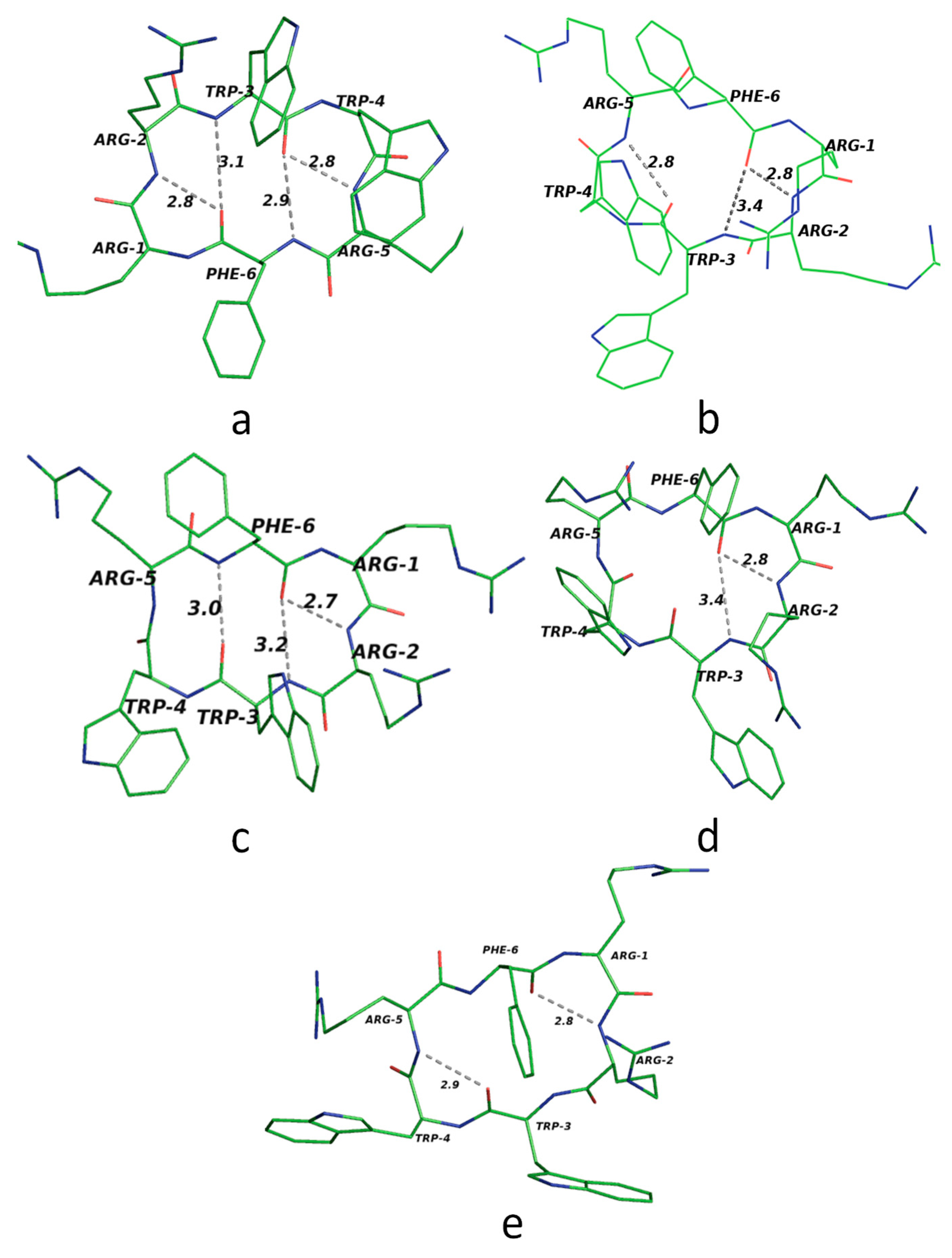
In their study, Ramakrishnan et al. [10] found that, besides the above criteria, different hydrogen bonds stabilize peptides. They identified these bonds by utilizing stereochemical studies and energy calculations. Using the minimization technique on these peptides, they showed the presence of different hydrogen bonds with secondary structural motifs like beta turns and gamma turns. According to their results, there are various bonds that occur like the bifurcated bond between amino acid residues 4-1 and 3-1 with type I or the inverse type. Similarly, for the type II beta turn, the same acceptor oxygen forms hydrogen bonds. There are also parallel bonding patterns seen in between amino acid residues like 3N-6O and 6N-3O [12].

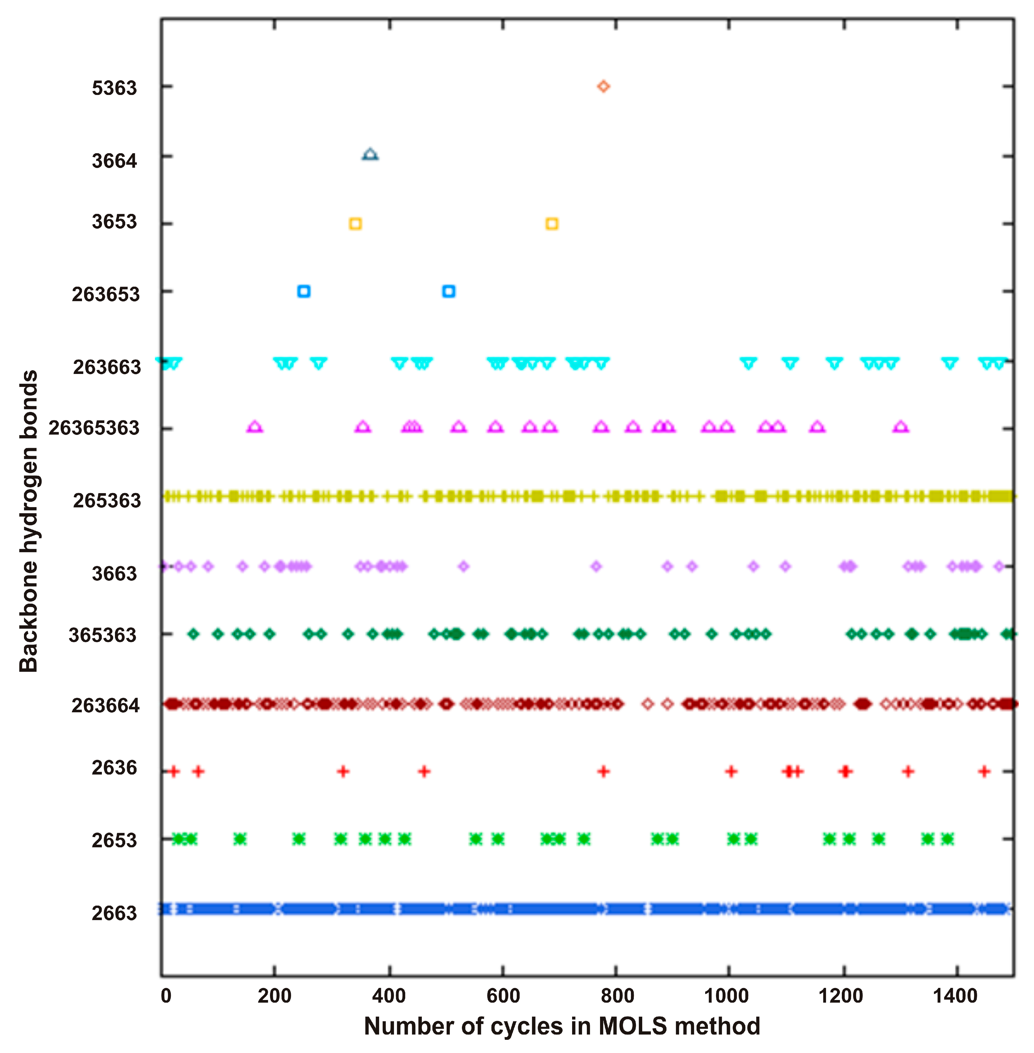
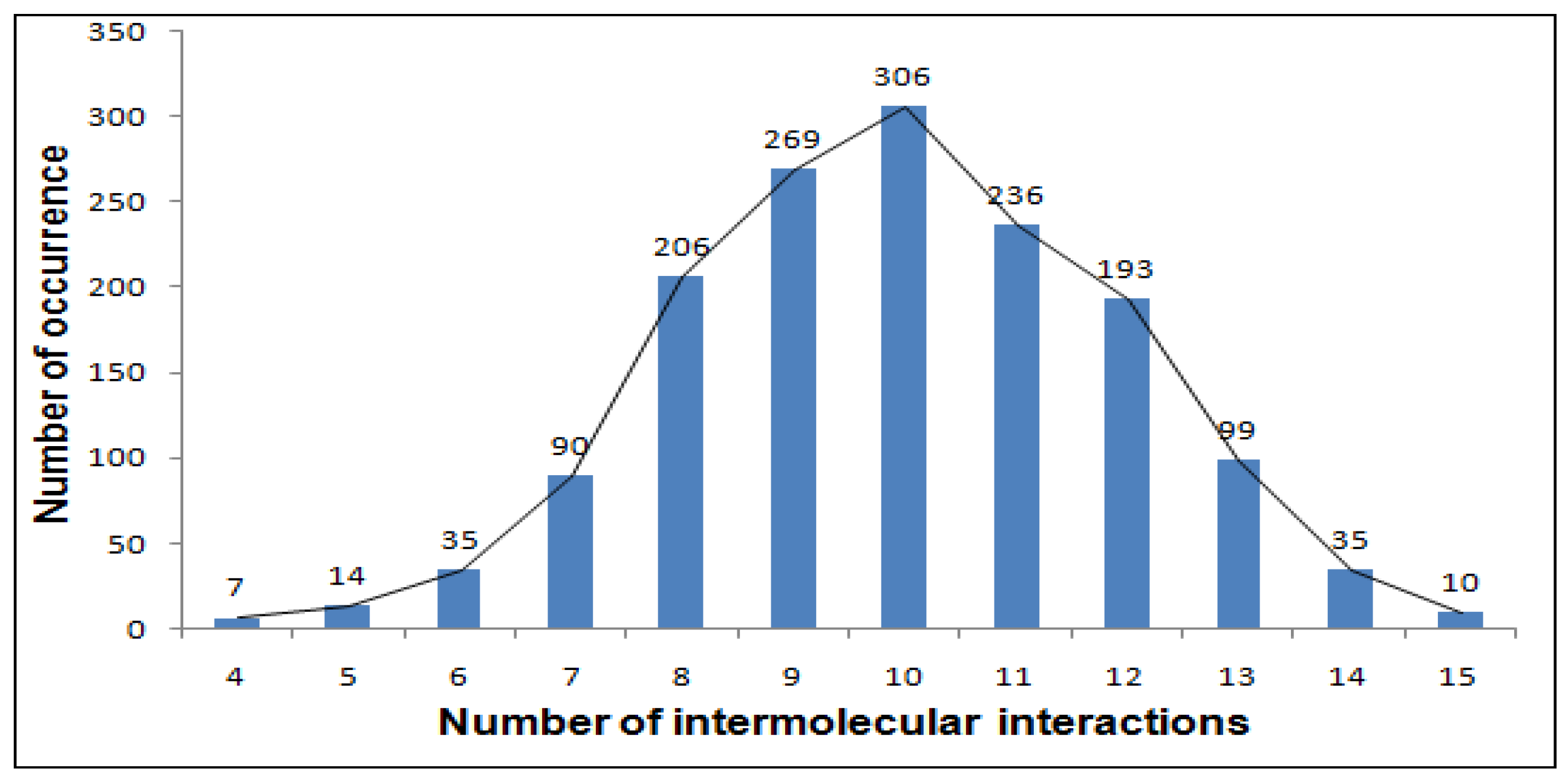
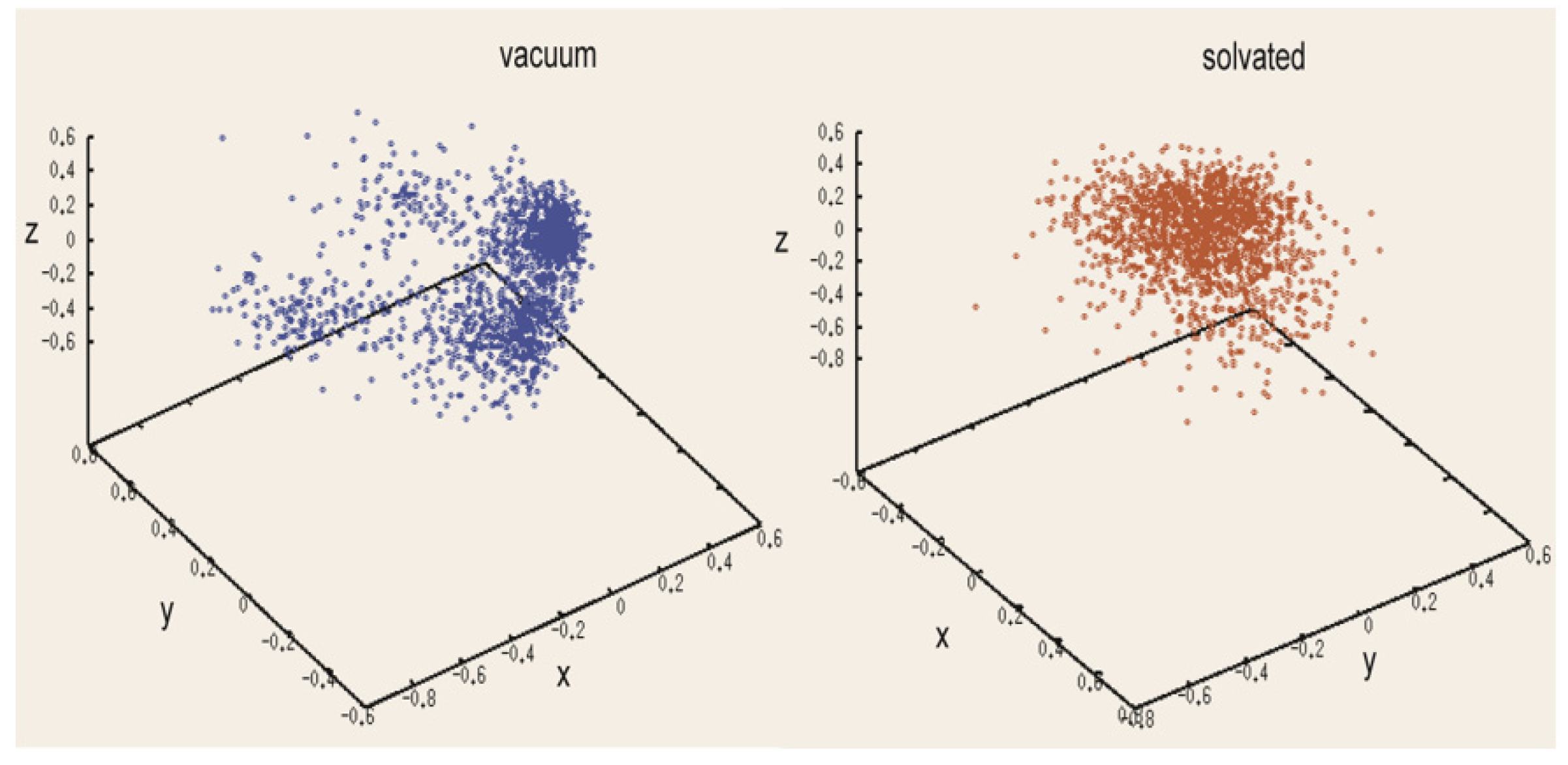
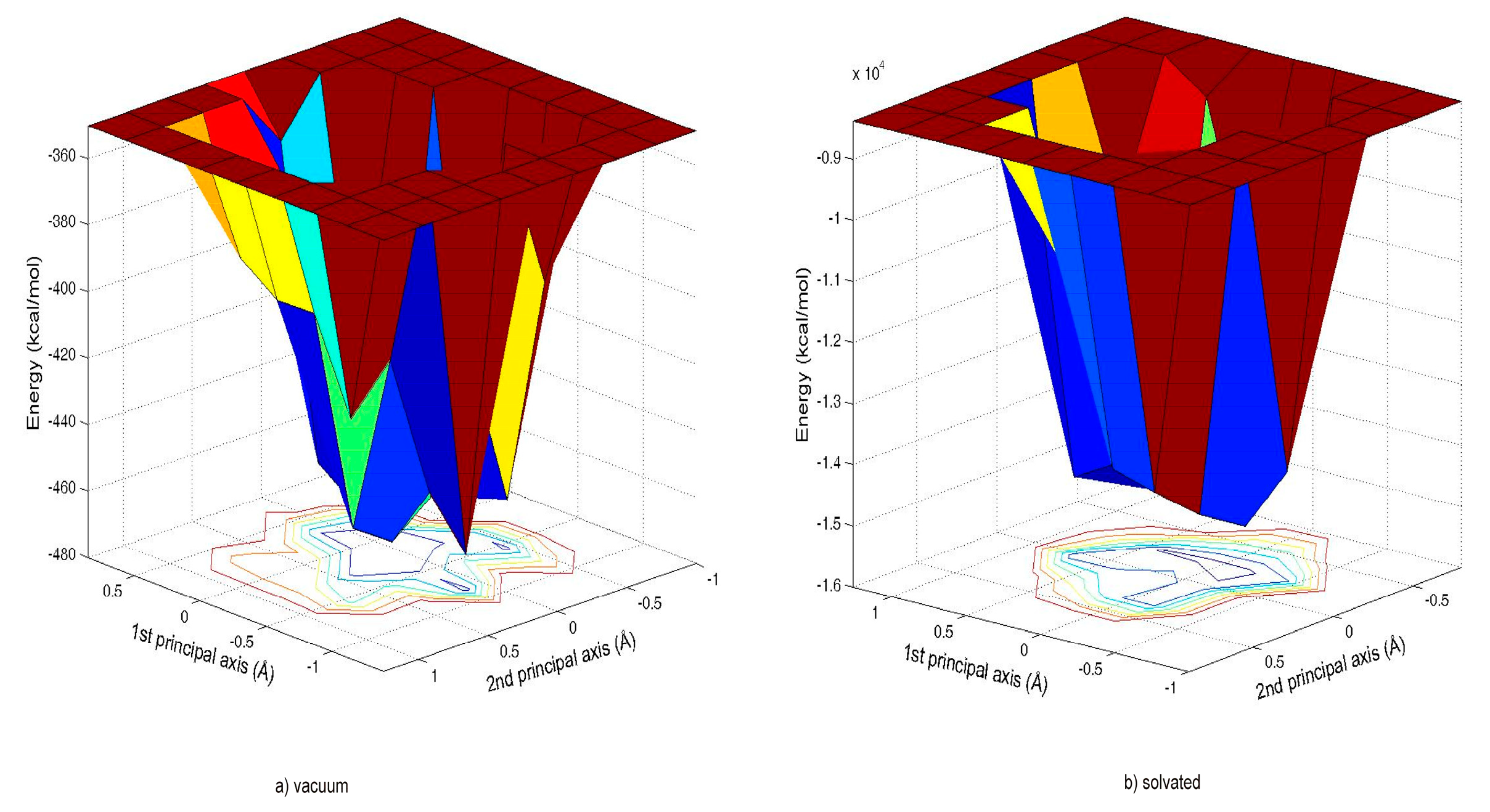
We investigated the cyclic hexapeptide of an antimicrobial peptide with the sequence RRWWRF in the current study. Here, the amino acid residues do not have similar patterns, and so we took this as a test case. We used the solved NMR structure from the PDB databank with id 1QVL [13]. We took the best model as the input for our MOLS algorithm. To investigate conformational variations, we explored the conformation of this peptide in a vacuum and with an explicit solvent. This served as a preliminary study for our mean field technique, MOLS. We present a comprehensive account of the peptide’s conformational energy landscape, meticulously detailing its features within an explicit water environment. We also describe the various secondary motif structures and the backbone hydrogen bonding patterns, along with their effects on the environment. The Materials and Methods Section describes the addition of explicit water molecules and interaction energy calculations. Then, the results obtained for each are compared.

2. Materials and Methods

One of the methods used to thoroughly investigate the conformational space of oligopeptides is the mean field technique (MFT) when it is combined with MOLS sampling. The mean field technique (MFT) along with MOLS sampling was previously employed by researchers on the ECEPP3/and AMBER force fields, but the inclusion of solvent molecules was disregarded. A detailed explanation of this method was already outlined in [14,15] and is also available at https://shodhganga.inflibnet.ac.in/handle/10603/198217, accessed on 18 April 2025. This method’s application in this study is described as follows.

This technique divides the conformational space into a number of subspaces, each containing numerous states. The effective potential obtained by setting a unique subspace to a particular state is conducted by taking the probability weighted average of the pairwise interactions in the subspace and comparing it to that of the states in all other subspaces. Initially, this method sets equal probabilities for all states within a given subspace; these probabilities are then recalculated using the Boltzmann function of the effective potential. The next cycle involves recalculating effective potentials using the new probabilities. We repeat this iterative procedure until the probabilities converge. The subspace with the highest probability after convergence will be the optimum one in the conformational space. For example, if we apply this method to determine the protein backbone conformation, then each of the backbone torsion angles will be considered the subspace, and the values that it can attain will be from 0 to 360°. Other consecutive states in steps of 10° can be accessed, but the effective potential cannot simply be calculated as the weighted sum of pairwise interactions because one of the torsion angles is set to such a value. If one sets the values for a pair of torsion angles, the occurring interactions will also depend on all the intermediate torsion angles. Calculating the potential is rigorous and requires considering all torsion angles, leading to a combinatorial explosion [14,15].

Using MOLS sampling, which tackles the small conformational space sample size, simplifies calculating the effective potential, easing the complexity of the problem. This method is used in the design of agricultural and clinical trials [16]. Usually, this involves identifying a small representative sample of a multivariable experimental space. We perform these calculations on this subspace instead of the whole space. A Latin square of order m is the arrangement of m symbols in an m × m square matrix in such a way that each symbol occurs exactly once in every row and once in every column [15]. A simple Latin square of order 3 is shown in Figure 1. This example uses the letters of the Latin alphabet (A, B, C) as symbols to construct the square [14,15]. Two Latin squares of order m are called orthogonal if, when one is superimposed on the other, all m² possible combinations of the two sets of m symbols are present and each symbol of the one square occurs once and only once, with the symbols of the other squares being present. 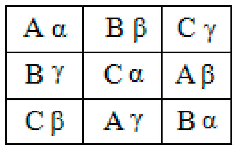Figure 2 shows a pair of orthogonal Latin squares involving two sets of three elements each [14]. This pair was constructed by the superposition of two Latin squares, one square containing Latin letters (A, B, C) and the other constructed with Greek letters (α, β, γ). Figure 2 shows that each subsquare contains one Latin and one Greek letter, and each letter combination appears only once. The symbols are arranged so that all m² pairs appear in the array [14,15]. Upon extending this concept to N mutually orthogonal Latin squares (MOLS), every pair is orthogonal. In the example of three MOLS (m = 3), the first square is orthogonal to the second and third squares, and the second is orthogonal to the third. The construction of a complete set of m-1 mutually orthogonal Latin squares of order n is shown to be possible if m is a prime number or an integer power of a prime [14,15,16].

A single Latin square of order m allows one to investigate the effects of setting three subspaces, each at the m different states in only m² trials instead of the m³ trials that would be required for a complete and exhaustive search of the sampling. A set of n mutually orthogonal Latin squares of order m allows one to investigate the effects of setting n factors to m different values, again in only m² (instead of mⁿ) trials. The above description shows that a distinctive feature of using MOLS to select sample points is the sample’s inclusion of every possible pairwise setting of all states of all subspaces [14,15,16].

When applying this method to the exploration of conformational spaces, including the protein mapped out by the backbone torsion angles of a peptide chain, we identify subspaces with torsion angles, where there are n such angles, as well as identifying states as the values that the torsion angles can take, where there are m such values accessible to each torsion angle. Out of a total of mⁿ points available in the conformational space, we select n² points using MOLS and calculate the potential energy corresponding to each of these conformations. In order to calculate the effective potential realized from setting the torsion angle to a specific value, we take the Boltzmann-weighted average of the potential energies at these points in the MOLS grid at which the set value of the torsion angle appears. We note that, as described above, this ensures the pairwise sampling of the set value of the torsion angle with every value of every other torsion angle. We repeat this procedure for all values of all torsion angles, using the same MOLS grid specifying the m² conformations. At the end of this set of calculation, we obtain the effective potential corresponding to every set value of each torsion angle. In the routine MFT procedure, these potentials are used to recalculate probabilities, which are used to recalculate the effective potential in iterative cycles until it converges [14]. In the present method using MOLS sampling, however, this is not possible since the effective potential is itself calculated as a Boltzmann-weighted average of the potential calculated in the MOLS grid. Thus, we use the effective potentials at the end of one round of calculations described above directly as substitutes for the final probabilities. For each torsion angle, we consider the value with the lowest effective potential the most probable one; the set of the most probable values for all torsion angles defines the optimum conformation of the peptides [14,15].

A crucial assumption underlying the MFT procedure, in particular when used with MOLS sampling, is regarding the degree of independence of the variables. The procedure works best when the variables are completely independent of each other; however, in that case, they are not required, and a few simple one-dimensional searches would quickly identify the optimum.

Backbone torsion angles are highly interdependent, and the procedure outlined above may not lead always to a single global optimum. The second assumption implicit in the procedure is that such a single global optimum exists on the potential energy landscape. In fact, as many studies have shown, most definitions of the force field operating in proteins and peptides describe the presence of several optima (minima) in the conformational space with approximately equal energy values. This method is an efficient way of exploring the entire space in an exhaustive manner and identifying all the optima. The construction of a single MOLS grid of order m, as described above, results in one optimal or low-energy conformation. Repeating this procedure by using a unique set of MOLS leads to another set. There are (m!)ⁿ different ways of constructing the MOLS grid [15]; in principle, the calculations may be repeated as many times as possible to repeatedly obtain all low-energy conformations. This does not mean that there are (m!)ⁿ low-energy conformations for a peptide. The conformations generated in the preceding cycles are obtained as they were in the previous process.

The well-known Met-enkephalin test case proved the usefulness of this method; the procedure, repeated over a few hundred cycles, exhaustively identified all minima. The energies of the experimental structure and the theoretical structure also fall within the range of the energies generated by this method. Some structures were also present with an energy that had not been seen anywhere else before. In the abovementioned method, we used the ECEPP/3 semi-empirical force field, without including explicit water molecules [14,15].

In the present work, we implemented our method for cyclic peptides. Here, we used the input as the selected structure. The program was changed so that the user could provide their own built structure as the input. Here, we used the antimicrobial cyclic hexapeptide PDB ID 1QVL as the test case [13]. The cyclic nature of the peptide backbones means that the first and last terminals of the linear peptide fuse to form a peptide bond, eliminating main chain rotation. We applied rotations to the side chains and then generated an optimized structure using two different environments, in the presence and in the absence of an explicit solvent. We used the VMD program [17] to explore both environments. We added explicit water molecules to each of the defined n2 MOLS conformations by placing a solvent box using the VMD program. We solvated the peptide using TIP3P water molecules, extending the water approximately 10 Å in each direction from the molecule’s ends. When the side chains of the peptide were in or out of plane, it was ensured that the solvent molecule always covered them. After this, we calculated the conformational energy of the peptide structure using the CHARMM22 potential [18]. The calculation of the total energy involved the summation of several energy terms, namely, the torsion angle energy, the energy from electrostatic interactions, the van der Waals energy, and the energy associated with intermolecular interactions. The MOLS method involved obtaining effective energies for each conformational variable value based on the calculated potential energy of the n² molecule, in order to identify the optimal conformation associated with it. We solvated the obtained optimal conformation using the same procedure and removed the conformational constraints by performing 1000 steps of conjugate gradient minimization using the NAMD minimization procedure [19]. In the minimization process, the energies of bond length, bond angle, and torsion angle and the improper nonbonded energies were taken into account. We did not use water–water interaction terms. Furthermore, a separate set of 1500 conformations was generated for the peptide, which was devoid of water molecules and subjected to a vacuum environment. Computation was conducted to generate one structure with and without a solvent using an AMD Opteron processor at 2.2 GHz for 57 min and 10 min, respectively.

3. Results

Utilizing the MOLS method, we investigated the conformational changes in the antimicrobial cyclic hexapeptide (RRWWRF) both in the presence and absence of explicit solvent molecules, analyzing the impact of solvation on its structure. The structure with the lowest energy, derived from both sources, was presented by us, after which we conducted an analysis of the motifs and their distributions. Furthermore, our analysis included an examination of conformational flexibility, which was determined using backbone bonding patterns; in the case of explicit solvation, we also described the interactions between the peptide and the surrounding water molecules. In this report, we investigate and document the influence the solvent has on the energy landscape of the system.

3.1. The Minimum Energy Structure

A visual representation of the global structure, as derived from the application of the MOLS method, is presented in Figure 3. As illustrated in Figure 3a, the most stable structure is characterized by a 2.97 Å bond that links the nitrogen of phenylalanine 6 (6Phe N) to the backbone oxygen of tryptophan 3 (3Trp O), thus contributing to its stabilization. Unlike in the experimental structure, the side chains differ; there are three Arg residues with donors stabilized by backbone interactions (Figure 3a), resulting in the lowest energy of −501.15 kcal/Mol, as expected. An analysis of structural variation shows backbone and heavy atom rmsd values of 0.48 Å and 4.09 Å, respectively, between the experimental and lowest-energy structures. In Figure 3b, we observe the lowest-energy structure in water molecules; it has a backbone interaction similar to that of the experimental structure in between 6Phe and 3Trp O. The side chain of the Arg residues is bonded with the oxygen atoms of the solvent molecules, and thus, they are stretched outside of the plane of the backbone atoms, leading to less of a structural difference from the experimental structure by having an rmsd of 0.38 Å with respect to the backbone atoms and a deviation of 2.83 Å with respect to the heavy atoms with an energy value of −19,182.78 kcal/Mol.

As detailed in our previous publications, the lowest-energy structure identified from the range of structures investigated is rarely the most accurately sampled, a consequence of the conformational differences between this theoretically derived minimum energy state and experimentally observed structures. The findings presented in this work corroborate previous research [14,15], further solidifying the validity of this assertion. We found structures that are very close to the experimental ones with respect to the rmsd of heavy atoms, and Figure 4 shows these conformations. Figure 4a shows the structure obtained without a solvent, exhibiting a 3.65 Å deviation. This structure has a large rmsd because it has an additional bond in between the backbone atoms 2Arg N and 6Phe O; this makes the backbone of the residue 1Arg to move out of the plane to that of the experimental structure, and its energy is −447.54 kcal/Mol. Figure 4b shows the structure that has an rmsd of 1.65 Å, which was obtained from the solvated structure. The solvated structure, as expected, has a lower rmsd value than the vacuum structure; its backbone is nearly identical, possessing the same stabilizing bonds as the experimental structure (backbone hydrogen bonds omitted for clarity), and its energy is −13,523.22 kcal/Mol.

3.2. Structural Motifs

Extensive research on cyclic hexapeptides has already demonstrated the typical adoption of a trans configuration for all their peptide linkages. Due to the nature of peptide linkages, the resulting conformation includes two beta folds. In order to visualize the beta folds present in each of the 1500 conformations produced through the application of the MOLS method, considering both vacuum and solvent environments, we employed PROMOTIF software [20] for the purpose of identifying beta and gamma folds by meticulously analyzing the frequency of secondary structural motifs. In defining the beta folds, we utilized a contiguous sequence of four amino acid residues which are 7 Å long. The classification of a fold as a beta turn is contingent upon the presence of a hydrogen bond within its structure; this hydrogen bond serves as a crucial defining feature that distinguishes beta turns from other types of folds. When considering a sequence of three consecutive amino acid residues, specifically those designated as i, i + 1, and i + 2, it is possible for a hydrogen bond to form between the first residue in this sequence (i) and the third residue (i + 2), as shown in

Table 1. Classic and inverse turns.

Turn Type	φ (i + 1) (deg)	ψ (i + 1) (deg)
Classic	75.0	−64.0
Inverse	−79.0	69.0

and

Table 2. The distribution of beta folds for the cyclic peptide in the two environments of interest.

Type of Beta Motif	Vacuum				Total	Solvated				Total
	Turns		Bends			Turns		Bends
	1234	3456	1234	3456		1234	3456	1234	3456
II’	-	410	-	10	420	-	1050	-	21	1071
IV	-	998	9	77	1084	-	378	5	42	425
Total	-	1408	9	87	1504		1428	5	63	1496

. Among the 1500 generated structures analyzed, 1496 were explicit solvated structures, comprising 1428 beta turns, and the remaining structures were beta bends and beta folds. Meanwhile, among the non-solvated structures, 1504 had beta folds, and among them, 87 were beta bends, and the rest were turns. Table 2 shows that the beta motifs are nearly identical in both systems; however, the difference lies in the intramolecular interactions occurring during turn formation. Explicit solvation strongly favors the 3456 beta II′ turn, which occurs approximately 2.56 times more frequently than it does in non-solvated structures. The type IV beta turn of 3456 occurs the most in the non-solvated system, and it occurs 2.64 times more frequently than it does in solvated structures. In the present case, the II′ beta motif is the most common in the solvated structure compared to the non-solvated one, and this is as observed in the experimental results mentioned [13].

Table 3. The distribution of gamma turns for the cyclic peptide in vacuum and in the presence of an explicit solvent.

Type	Vacuum					Solvated
	123	234	345	456	Total	123	234	345	456	Total
Inverse	2	-	-	63	65	-	-	-	11	11
Classic	-	-	575	-	575	-	-	92	-	92
Total	2		575	63	640	-	-	92	11	103

shows the occurrence of gamma turns. Explicit solvation decreases the occurrence of turns compared to non-solvated structures. There are six times more occurrences of gamma turns in the non-solvated structures than there are in the solvated ones. In both cases of the conformational search, single- and double-beta folds and gamma folds occur. This shows that the occurrence of double-beta folds is less likely, as shown in

Table 4. The frequencies of single- and double-folded structures for the cyclic peptide.

Type	Vacuum			Solvated
	Single Fold	Double Fold	Total	Single Fold	Double Fold	Total
Beta	1488	8	1496	1490	3	1493
Gamma	640	-	640	103	-	103
Total	2128	8	2136	1593	3	1596

. Figure 5 shows such a double-beta fold structure obtained from non-solvated structures, and it has a 1–4 type IV bend and also a 3–6 type IV bend, and there are no gamma turns. The solvated structure shows two beta folds, as illustrated in Figure 6; one is a 1–4 type IV bend, and the other is a 3–6 type II′ bend. The non-solvated structure has both type IV and II′ folds, but the solvated structure only has type IV and type II′ beta double folds.

Table 5. The distribution of both beta and gamma motif structures for the cyclic peptide.

Type	No. of Structures
	Vacuum	Solvated
Single β fold, classic γ turn	575	92
Single β fold, inverse γ turn	63	11
Double β folds, inverse γ turn	1	-

displays the additional structures we observed, which include combinations of beta folds and gamma turns. This again demonstrates that the non-solvated structures yield more of these combinations than the solvated structures.

3.3. Hydrogen Bonds

We analyzed the intramolecular hydrogen bonds in both instances, with a theoretical explanation provided by Ramakrishnan et al. (1985) [12]. They thoroughly explained the potential backbone interactions of cyclic peptides, ranging from tripeptides to polypeptides. Figure 7 shows a possible hydrogen bonding pattern for the structures obtained without a solvent. Figure 7a illustrates a molecular structure with all backbone hydrogen bonds, resulting in a total energy of −440.20 kcal/mol; these bonds specifically connect residues 2N-6O, 3N-6O, 5N-3O, and 6N-3O. Figure 7b shows the three backbone bonding patterns, and a bond exists between 2N-6O, 3N-6O, and 5N-3O. There is a beta motif in the 3456 residue and a classic gamma turn at 345 with energy −470.13 kcal/mol. Figure 7c, illustrates a distinct structure featuring three bonds between 2N-6O, 3N-6O, and 6N-3O. Figure 7d shows a bond between 2N-6O and 3N-6O, with the motif being a beta fold at 3456 and a gamma turn of the inverse type at the 456 residue. Figure 7e shows two backbone hydrogen bonding patterns between the backbone atoms of 2N-6O and 5N-6O; this pattern also appeared in an earlier report by Ramakrishnan et al., showing a beta turn and a classic type IV gamma turn at residue 3456 and a classic turn at residue 345. These pictures show the overall variation in backbone bonding patterns and motifs. Steric hindrance avoidance, primarily stemming from interactions between a residue’s side chain and the preceding main chain carbonyl oxygen, leads to distorted conformations, as these interactions are largely determined by the residue type and its specific side chain [21].

Figure 8a–e illustrate the diverse array of backbone hydrogen bonds observed within the solvated peptide structures. In contrast to the non-solvated conformations, which exhibit a different number of hydrogen bonds, the solvated conformations are characterized by a maximum of three hydrogen bonds. As depicted in Figure 8a, the backbone bonding pattern among the 3N-6O, 5N-3O, and 6N-3O residues demonstrates the presence of a stabilizing antiparallel bonding interaction that is formed between residues 3 and 6. As shown in Figure 8b, the backbone bonding pattern of 2N-6O and 5N-3O is consistent with observations from prior studies. This structure contains a secondary motif composed of a type IV beta fold and a classic gamma turn involving residues 3456 and 345, respectively, a pattern also observed in Figure 8a. Figure 8c displays a 3456 beta II′ fold secondary motif, with hydrogen bonds 3N-6O and 6N-3O and an additional parallel bond with an explicit solvent molecule. Figure 8d illustrates a structure containing two hydrogen bonds (5N-3O and 6N-3O), lacking a gamma turn, and exhibiting only a type IV beta fold within residue 3456. A beta fold at residue 345 (type IV) and an inverse gamma turn at residue 456, along with two hydrogen bonds (3N-6O and 6N-4O), are shown in the structure (Figure 8e).

We investigated the combination of backbone hydrogen bonds along the conformational cycles of the MOLS method for solvated and un-solvated structures to determine the solvent-favored backbone hydrogen bonding pattern. Figure 9 shows the occurrence of all bonds for non-solvated structures. This figure shows 13 different combinations of backbone bonding patterns. Figure 10 shows eight such bonding patterns for the solvated structures. The most favored non-solvated bonding patterns (2N-6O and 6N-3O) are not favored in the solvated structures. In the non-solvated structures, the most favored bonding patterns, in addition to those previously discussed, include 2N-6O and 5N-3O; further analysis reveals that among the two- and three-bond combinations, the 2N-6O, 3N-6O, and 6N-3O bonds show a significantly greater contribution to the non-solvated structures compared to their solvated counterparts. The bonds between the nitrogen and oxygen atoms in the molecules 3N-6O, 5N-3O, and 6N-3O exhibit identical bonding characteristics. An analysis of the backbone bonding patterns reveals nearly identical occurrences of the 2N-6O–3N-6O and 3N-6O–6N-3O bonds, regardless of solvent presence. From the bonding pattern, it is shown that the solvate structure’s distinct feature is its preference for the 5N-3O and 6N-3O backbone bonding patterns, bifurcating from residue 3 to residues 5 and 6, respectively. The bonding pattern indicates a lower probability of backbone hydrogen bond formation in the solvated structure compared to the non-solvated structure.

3.4. The Intermolecular Interaction

In the solvated structures, the interaction of water molecules throughout all the generated conformations is analyzed. Figure 11 displays the occurrences of possible intermolecular interactions between explicit water and the peptide. We observed that the number of interactions varied between 4 and 15, averaging at 10, which represents the most frequent occurrence. Figure 12 depicts the structure exhibiting the minimum (a) and maximum (b) number of intermolecular interactions. Reduced water molecule interactions cause Arg residue side chains to interact with main chain atoms to stabilize. Increased water molecule interactions cause all Arg residue donors to interact with water molecules, pulling them away from the backbone plane. Fluctuations in water molecule count lead to diverse backbone interactions, enabling structural flexibility and specific backbone bonds to achieve a lower energy state, as confirmed by the experimental results showing flexibility in this cyclic peptide with water.

3.5. Energy Landscape

Determining the peptide potential energy landscape allows researchers to understand the dynamic nature of peptides and explore various conformations in different kinetic states. Representing the peptide landscape with only two or three states is not ideal; a folding funnel model is a better representation of the folding pathway. Small oligopeptides have considerable conformational flexibility as their degrees of freedom are not limited. The energy landscape is represented as a multidimensional surface, consisting of states, peaks, and local minima. Using the MOLS method, we explore conformational variables and degrees of freedom to create the potential energy landscape; each generated structure is minimized to its nearest minimum, and then the landscape is constructed. The landscape’s complexity stems from the peptides’ conformational flexibility, as previously discussed. To solve this, the problem is reduced from a multidimensional to a low-dimensional space. These reduced dimensions should provide almost all the characteristics of the landscape. We applied a similar procedure to that used by Levy and Becker [22,23,24]. This method reduces the multidimensional space to a low-dimensional space with the help of a principal component analysis (PCA). The implemented PCA is the so-called principal coordinate analysis (PCoorA). In cyclic peptides, rotations occur from the side chains due to the closed-ring form of the backbone. This conformational constraint reduces the flexibility of the molecule and thus the volume of the conformational space. Here, we observed the flexibility attributed to the environment of the peptide. Figure 13 shows a plot of the first principal component versus the second principal component analysis, while the left side shows the structures generated in vacuum and the right the solvated one. The volume of spread for the vacuum structure is greater compared to the solvated one. This indicates that the non-solvated structure has a larger group of similar conformations, thus exhibiting greater flexibility. This is also evident in the greater number of backbone bending patterns, as previously discussed. The spread of the data seems to be smaller in the solvated structures, and the structures are almost close to each other, thus leading to a more restricted backbone bonding pattern than that of the non-solvated structures. Under these conditions, the variance of the two axes in vacuum is 10% more than that in the solvated condition. We also explored the energy landscape with respect to the two principal axes. The representation of a 3D topographical map displays the local minima and is thus called the minimum envelope representation, as referred to by O. M. Becker (1998) [24]. Figure 14 shows a 3D topographical energy map of the vacuum (a) and the solvated (b) peptide. This figure shows the presence of a broad funnel structure. In the case of the map for the non-solvated structures, the funnel seems to be rugged, and the bottom of the deep basin does not contain only a single dominating structure, as it has many when compared to those of the solvated form. In the case of the solvated peptide, the landscape is smooth; this shows the effects of solvent interactions and their ability to maintain structures with defined backbones and folds, as seen in the experimental structure, but there is minor flexibility due to different backbone interactions occurring. The local minima in the solvent seem confined in a particular region.

4. Conclusions

In this study, the MOLS method was used to explore the conformational energy landscape of peptides, which are not constrained. We reported that this sampling method explores all possible local minima of a given sequence. In the current study, we took a cyclic hexapeptide and examined its conformations in the presence and absence of an explicit solvent. The solvated peptide closely matched the experimental results, with a lower heavy atom RMSD than that of the un-solvated form. A further analysis of secondary motif presence revealed entirely distinct patterns in the non-solvated and solvated structures. As expected, the solvated structures show fewer gamma turns. Solvation also reduced the number of possible backbone hydrogen bonding patterns in the peptide, resulting in altered side chain orientation. In conclusion, to determine the cyclic peptide’s structure, the nature of the environment is important. The conformations obtained from the MOLS method will be a good starting structure for molecular simulation and for further mutational studies to enhance the properties of antimicrobial peptides.

References

1. Kessler, Η. Conformational and biological activity of cyclic peptides. Angew. Chem. Int. Ed. Engl. 1982, 21, 512–523. [Google Scholar] [CrossRef]
2. Ovchinnikov, Y.V.; Ivanov, V.T. Proteins; Neurath, H., Hill, R.L., Eds.; Academic Press: New York, NY, USA, 1982; Volume 5, p. 307. [Google Scholar]
3. Karle, I.L.; Karle, J. Conformation of cyclo(Gly-L-Pro-L-Pro-Gly-L-Pro-L-Pro)2Mg2+ complex crystallized from C2H3CN solution. Proc. Natl. Acad. Sci. USA 1981, 78, 681–685. [Google Scholar] [CrossRef] [PubMed]
4. Ramakrishnan, C.; Narasinga Rao, B.N. Stereochemical studies on cyclic peptides. Int. J. Pept. Protein Res. 1980, 15, 81–95. [Google Scholar] [CrossRef] [PubMed]
5. Groth, P. Crystal Conformation of Cyclotrisarcosyl at −160 degrees C. Acta Chem. Scand. 1976, A30, 838. [Google Scholar] [CrossRef]
6. Venkatachalam, C.M. Stereochemical studies on cyclic peptides. II molecular structure of cyclotriprolyl. Biochim. Biophys. Acta 1968, 168, 397. [Google Scholar] [CrossRef]
7. Manjula, G.; Ramakrishnan, C. Stereochemical studies on cyclic peptides. IX. Conformational studies on cyclic tetrapeptides containing alternating cis and trans peptide units. Biopolymers 1979, 18, 591–607. [Google Scholar] [CrossRef]
8. Groth, P. Crystal Structure of Cyclotetrasarcosyl. Acta Chem. Scand. 1970, 24, 780. [Google Scholar] [CrossRef]
9. Manjula, G.; Ramakrishnan, C. Stereochemical studies on cyclic peptides. Int. J. Peptide Protein Res. 1979, 13, 353. [Google Scholar] [CrossRef]
10. Ramakrishnan, C.; Narasinga Rao, B.N. Conformation in Biology; Srinivasan, R., Sarma, R.H., Eds.; Adenine Press: New York, NY, USA, 1982; p. 141. [Google Scholar]
11. Mauger, A.B.; Stuart, Ο.Α.; Highet, R.J.; Silverton, J.V. Synthesis of an actinomycin-related peptide, cyclo-(Thr-D-Val-Pro-Sar-MeAla), and conformational studies by nuclear magnetic resonance and x-ray crystallography. J. Am. Chem. Soc. 1982, 104, 174. [Google Scholar] [CrossRef]
12. Ramakrishnan, C.; Paul, P.K.C.; Ramnarayan, K. Cyclic peptides––Small and big and their conformational aspects. J. Biosci. 1985, 8, 239–251. [Google Scholar] [CrossRef]
13. Appelt, C.; Wessolowski, A.; Söderhäll, J.A.; Dathe, M.; Schmieder, P. Structure of the Antimicrobial, Cationic Hexapeptide Cyclo(RRWWRF) and Its Analogues in Solution and Bound to Detergent Micelles. Chembiochem 2005, 6, 1654–1662. [Google Scholar] [CrossRef] [PubMed]
14. Vengadesan, K.; Gautham, N. Conformational studies on enkephalins using the MOLS technique. Biopolymers 2004, 74, 476–494. [Google Scholar] [CrossRef]
15. Vengadesan, K.; Gautham, N. Enhanced sampling of the molecular potential energy surface using mutually orthogonal Latin squares: Application to peptide structures. Biophys. J. 2003, 84, 2897–2906. [Google Scholar] [CrossRef]
16. Finney, D.J. Randomized blocks and Latin squares. In Experimental Design and Its Statistical Basis; Cambridge University Press: London, UK, 1955; pp. 45–67. [Google Scholar]
17. Humphrey, W.; Dalke, A.; Schulten, K. VMD–Visual molecular dynamics. J. Mol. Graph. 1996, 14, 33–38. [Google Scholar] [CrossRef]
18. MacKerell, A.D., Jr.; Bashford, D.; Bellott, M.L.; Dunbrack, R.L., Jr.; Evanseck, J.D.; Field, M.J.; Fischer, S.; Gao, J.; Guo, H.; Ha, S.; et al. All-atom empirical potential for molecular modeling and dynamics studies of proteins. J. Phys. Chem. B 1998, 102, 3586–3616. [Google Scholar] [CrossRef] [PubMed]
19. Phillips, J.C.; Braun, R.; Wang, W.; Gumbart, J.; Tajkhorshid, E.; Villa, E.; Chipot, C.; Skeel, R.D.; Kale, L.; Schulten, K. Scalable molecular dynamics with NAMD. J. Comput. Chem. 2005, 26, 1781–1802. [Google Scholar] [CrossRef] [PubMed]
20. Hutchinson, E.G.; Thornton, J.M. PROMOTIF—A program to identify and analyze structural motifs in proteins. Protein Sci. 1996, 5, 212–220. [Google Scholar] [CrossRef]
21. Hoffmann, R.W. Flexible Molecules with Defined Shape—Conformational Design. Angew. Chem. Int. Ed. Engl. 1992, 31, 1124–1134. [Google Scholar] [CrossRef]
22. Levy, Y.; Becker, O.M. Energy landscapes of conformationally constrained peptides. J. Chem. Phys. 2001, 114, 993–1009. [Google Scholar] [CrossRef]
23. Becker, O.M.; Levy, Y.; Ravitz, O. Flexibility, conformation spaces and bioactivity. J. Phys. Chem. B 2000, 104, 2123–2135. [Google Scholar] [CrossRef]
24. Becker, O.M. Principal coordinate maps of molecular potential energy surfaces. J. Comput. Chem. 1998, 19, 1255–1267. [Google Scholar] [CrossRef]
Figure 1. A Latin square of order 3.
Sci 07 00093 g001
Figure 2. Two Latin squares are shown, one with Latin letters A, B, and C and the other with Greek letters α, β, and γ. The second Latin square is orthogonal to the first. These are two mutually orthogonal Latin squares of order 3 obtained from MOLS sampling.
Sci 07 00093 g002
Figure 3. The lowest-energy structure obtained (a) in vacuum and (b) in the presence of water.
Sci 07 00093 g003
Figure 4. The superposition of the lowest heavy atom rmsd structures with that of the experimental structure (a) in vacuum and (b) in the presence of an explicit solvent.
Sci 07 00093 g004
Figure 5. The structure obtained in vacuum with two beta bends, with one being 1–4 type IV and the other 3–6 type IV.
Sci 07 00093 g005
Figure 6. One of the structures with two beta bends, with one being 1–4 type IV and the other 3–6 type II′ in water.
Sci 07 00093 g006
Figure 7. (ae) display the various hydrogen bonding patterns observed in a vacuum.
Sci 07 00093 g007
Figure 8. (ae) show the various possible hydrogen bonding patterns observed in the presence of the explicit solvent.
Sci 07 00093 g008
Figure 9. The various combinations of hydrogen bonding patterns seen among the structures generated in vacuum throughout the 1500 cycles of the MOLS method (If the y value is 2636, then there are two bonds in between the atoms of residues 2N-6O and 3N-6O).
Sci 07 00093 g009
Figure 10. The various combinations of hydrogen bonding patterns seen among the structures generated in the presence of an explicit solvent throughout the 1500 cycles of the MOLS method (If the y value is 2636, then there are two bonds in between the atoms of residues 2N-6O and 3N-6O).
Sci 07 00093 g010
Figure 11. The distribution of the number of structures generated in the solvent compared to the number of intermolecular interactions observed.
Sci 07 00093 g011
Figure 12. A stereo view of the structure, (a) showing an interaction with fewer water molecules and (b) showing an interaction with many more water molecules.
Sci 07 00093 g012
Figure 13. This figure shows the distribution of the three principal coordinates obtained for the 1500 cycles of the MOLS method in vacuum (left-hand side) and in the presence of the explicit solvent (right-hand side), where x, y, and z represent the 1st, 2nd, and 3rd principal axes, respectively.
Sci 07 00093 g013
Figure 14. The conformational energy landscape for the 1500 structures generated from the MOLS method in (a) vacuum and (b) in solvent. x and y represent the principal coordinates, and z represents the respective energy.
Sci 07 00093 g014