Optimization of the Archimedean Spiral Hydrokinetic Turbine Design Using Response Surface Methodology

Abstract

This research investigates enhancing the performance of an Archimedes screw-type hydrokinetic turbine (ASHT). A 3D transient computational model employing the six degrees of freedom (6-DOF) methodology within the ANSYS Fluent software 2022 R1, was selected for this purpose. A central composite design (CCD) methodology was applied within the response surface methodology (RSM) to enhance the turbine’s power coefficient ($C_p$). Key independent factors, including blade length (L), blade inclination angle ($\gamma$), and external diameter ($D_e$), were systematically varied to determine their optimal values. The optimization process yielded a maximum $C_p$ of 0.337 for L, $\gamma$, and $D_e$ values of 168.921 mm, 51.341°, and 245.645 mm, respectively. Experimental validation was conducted in a hydraulic channel, yielding results that demonstrated a strong correlation with the numerical predictions. This research underscores the importance of geometric design optimization in improving the energy capture efficiency of the ASHT, contributing to its potential viability as a competitive renewable energy solution in the pre-commercial phase of development.

1. Introduction

The increasing global energy demand presents significant challenges for sustainable development as traditional energy sources continue to strain the environment. This growing consumption of energy, coupled with the finite nature of fossil fuels, has intensified the need for cleaner, renewable energy alternatives [1]. Among these, hydrokinetic energy, which harnesses the natural kinetic energy of moving water, has emerged as a promising solution. Hydrokinetic power generation offers a different approach compared to traditional hydroelectric methods. Instead of relying on massive dams and water storage, these systems harness the natural flow of water. This distinction makes them a gentler option for the environment and allows them to be used in a wider range of water bodies [2,3].

Hydrokinetic energy can be extracted from natural and artificial water bodies such as rivers, canals, and ocean currents. These resources offer vast untapped potential for generating electricity in a sustainable manner. Specifically, hydrokinetic turbines, designed to capture energy from flowing water without extensive infrastructure, are playing a crucial role in advancing renewable energy technology [4,5]. One such innovation is the Archimedean spiral hydrokinetic turbine (ASHT), which is designed to operate efficiently in low-velocity water flows. Its simple yet effective design enables it to harness energy from currents in rivers, tidal flows, and artificial channels [6].

Other common hydrokinetic turbine technologies include horizontal-axis hydrokinetic turbines (HAHTs) and vertical-axis hydrokinetic turbines (VAHTs). HAHTs, which operate similarly to wind turbines, are known for their high efficiency in unidirectional and steady flow environments, with typical power coefficient of performance ($C_p$) ranging from 0.35 to 0.45 [7]. VAHTs, such as Darrieus and Savonius turbines, can operate in multidirectional flows and require less alignment with the flow direction but often exhibit lower $C_p$ values, typically between 0.2 and 0.35, depending on the design [8]. In comparison, ASHTs offer unique advantages for shallow or confined water bodies due to their compact geometry and low start-up velocity requirements. While their $C_p$ values are generally slightly lower than those of HAHTs, recent optimization efforts, including the present study, aim to bridge this gap, improving the ASHT’s competitiveness as a viable solution for decentralized and low-head hydrokinetic energy applications.

Currently, several relevant studies focus on the ASHT, examining design processes, numerical simulation, and experimental evaluation. It is important to note that this technology remains in the early stages of development, with limited studies specifically addressing the application of the Archimedean spiral in hydrokinetic contexts. Research on the ASHT has evolved primarily from earlier studies on the Archimedean spiral wind turbine (ASWT). For instance, in wind turbine applications, these foundational studies have provided valuable insights that have informed the initial design parameters of the ASHT, guiding its adaptation for hydrokinetic energy generation. For example, the ASWT’s performance has been analyzed at different blade inclination angles ($\gamma$). In this analysis, $\gamma$ was set at values of 65°, 60°, 55°, and 50° [9]. The highest $C_p$ observed was 0.22 at a tip speed ratio ($TSR$ or $\lambda$) of 1.71 when $\gamma$ was 50°. Labib and colleagues determined that the highest Cp values occurred at lower $TSR$ values [9]. Another comparative study examined two distinct ASWT configurations: one with blades fixed at a 60° angle and the other with variable blade angles of 30°, 45°, and 60° [10]. Applying computational fluid dynamics (CFDs) simulations, the study found that the turbine with variable-angle blades obtained a maximum $C_p$ of 0.226 at a $\lambda$ of 1.96, while the turbine with fixed-angle blades reached a maximum $C_p$ of 0.207 at a $\lambda$ of 1.57. This represented a 9.18% increase in $C_p$. Furthermore, the authors noted that the first and third blades played a crucial role in maximizing energy extraction, specifically in wind energy applications [9].

The performance assessment of ASHT has been the central point of numerous studies documented in the literature. Suntivarakorn et al. investigated their design and operation for low-head hydropower generation. The researchers optimized the blade geometry, specifically the number of blades and the diameter-to-length ratio. A spiral turbine with a 2/3 diameter-to-length ratio and three blades exhibited superior performance. This design reached its peak torque output at a water flow speed of 1 m/s and achieved an optimal efficiency of 48% [11].

Monatrakul and Suntivarakorn investigated the operation of spiral turbines with varying of $\gamma$ for low-head hydropower applications. CFDs were employed to analyze the impact of $\gamma$ (15°, 18°, 21°, and 30°) on turbine efficiency under different water velocities. The results indicated that a blade angle of 21° yielded the highest torque in free-flow conditions. However, when a collection chamber was incorporated, a blade angle of 30° resulted in the highest efficiency, significantly surpassing the performance of a conventional three-bladed axial turbine [12]. Rat et al. explored the adaptation of the Archimedes spiral turbine, traditionally used in wind energy, to generate electricity from the kinetic energy of small rivers and streams. The turbine was directly coupled to a permanent magnet synchronous generator (PMSG) to convert the mechanical energy into electrical power. The system (turbine and PMSG) was simulated using MATLAB/Simulink to analyze its performance under various water flow conditions. The results showed that the turbine exhibits a rapid response to changes in water flow, with the angular speed and torque quickly stabilizing [13]. Rajbanshi et al. numerically investigated the influence of water velocity on turbine performance. Their findings revealed that increasing the water velocity from 1 to 2 m/s led to a substantial increase in the generated force and torque, with values ranging from 6.498 N to 25.974 N and 0.0725 Nm to 0.291 Nm, respectively. However, this increase in power output was accompanied by a decrease in turbine efficiency, which dropped from 37.81% at the lowest velocity to 18.96% at the highest velocity [14]. Badawy et al. employed CFDs to simulate and design an ASHT. The authors selected five NACA series profiles: 4401, 4405, 65107, 4403, and 4407, to evaluate their performance based on a $TSR$ of two for a turbine blade with a NACA 4401 profile [15].

Monatrakul et al. investigated the performance of spiral turbines with different $\gamma$ (18° and 21°) for low-head hydropower generation. Laboratory experiments and field tests were conducted to evaluate the efficiency and power output of these turbines under various water flow conditions. The findings demonstrated that 21° achieved the greatest efficiency, especially when dealing with faster water flow. Moreover, integrating this turbine with a straight duct followed by a diffuser and a nozzle chamber emerged as the optimal arrangement, producing substantial power even in slower-moving water [16]. A study contrasting the performance of ducted (DASHT) and non-ducted (ASHT) Archimedes spiral hydrokinetic turbines was presented by Song et al., highlighting significant differences in their energy capture capabilities. The ASHT, inspired by technologies like the ASWT, operates efficiently at lower speeds due to the higher density of water, achieving a maximum $C_p$ of 0.237 at a $TSR$ of 1.5. In contrast, the DASHT demonstrates a remarkable improvement, reaching a maximum $C_p$ of 0.525 at a $TSR$ of 2.5, which represents a 122% increase in performance compared to the ASHT [6].

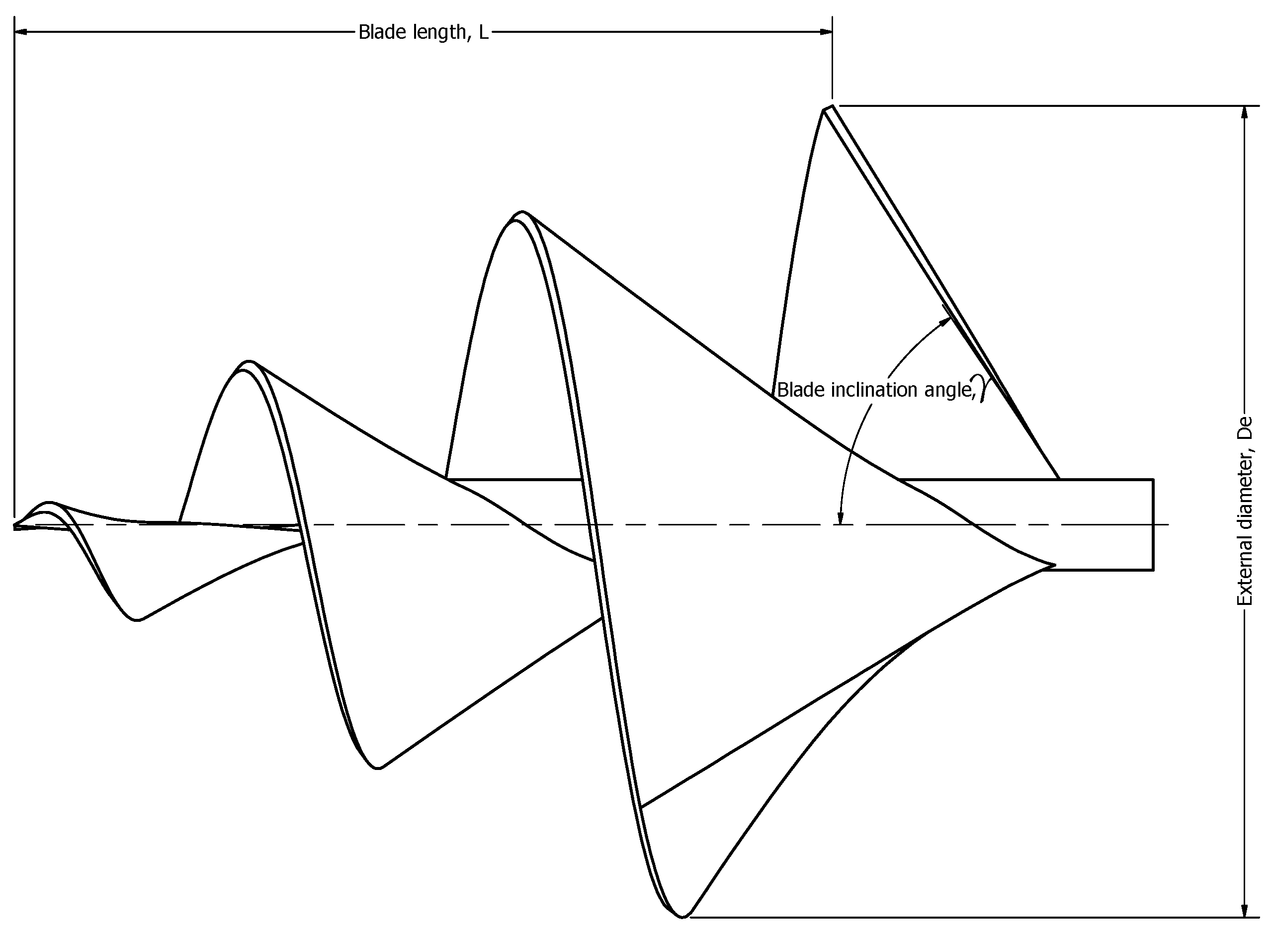
According to the literature review, the performance of ASHT is a function of its design parameters and operational conditions. Key parameters such as the diameter of the rotor, $\gamma$, the length of the blade, and the number of blades have a direct impact on the turbine’s energy-capturing efficiency. Therefore, the optimization of the turbine’s geometry is critical to maximize its power output and operational efficiency under different water flow conditions. Despite these insights, most existing studies have explored the influence of these parameters individually or through limited combinations. This research gap highlights the novelty of applying response surface methodology (RSM) to enhance the turbine’s efficiency by simultaneously optimizing three key geometric parameters: blade length (L), blade inclination angle ($\gamma$), and external diameter ($D_e$). This integrated approach provides a more comprehensive understanding of their combined effects on the power coefficient ($C_p$), which has not been thoroughly explored in previous research.

RSM, a widely recognized statistical approach, serves to optimize intricate systems influenced by numerous factors [17,18]. In this study, a central composite design (CCD) will be specifically employed as the experimental design framework. The CCD allows for the efficient exploration of the design space by systematically varying the turbine’s key parameters, thus generating data that help model the relationship between these factors and the turbine’s performance. One advantage of CCD is its ability to fit a quadratic model, which provides a more accurate representation of nonlinear effects in the system. Additionally, CCD requires fewer experimental runs than a full factorial design, which reduces both time and resource consumption. However, one disadvantage is that the quality of the model may be sensitive to experimental noise or inaccuracies in the measurement of responses, which can affect the reliability of the optimization results.

The novelty of this work also lies in the combination of statistical optimization with experimental validation, offering both a predictive and practical contribution to the field. Following the optimization process, the design resulting from the experimental methodology will undergo experimental validation in a controlled environment. The optimized turbine will be tested in a hydraulic channel, simulating real-world conditions to evaluate its performance. This experimental validation is crucial to ensure that the optimized design performs as predicted under actual operating conditions, providing a robust foundation for future real-world applications.

2. Methodology

2.1. Archimedean Spiral Hydrokinetic Turbines

The ASHT is a device designed to capture energy from the flow of water, such as rivers or tidal currents. The turbine’s helical, spiral-shaped rotor, inspired by the geometry of the Archimedean spiral, allows it to harness the kinetic energy of moving water efficiently. Unlike traditional water turbines, ASHTs can operate effectively in low-flow conditions due to their unique shape, which promotes smooth, continuous rotation even at low water velocities. This design makes ASHTs particularly suitable for hydrokinetic energy generation in decentralized or shallow water environments, contributing to sustainable energy solutions by leveraging natural water flow without the need for large-scale dams or infrastructure.

The ASHT comprises a cylindrical shaft which supports three equidistant blades, each with an external diameter ($D_e$) and a helical angle ranging from 0° to 360°. The blades are positioned at relative helical angles of 0°, 120°, and 240° in the angular displacement plane, ensuring uniform distribution around the shaft. The blade radius, represented as $D_e$/2, is defined as the vertical distance between the blade tip and the center of the rotating shaft. Prototypical ASHT models, specifically designed for the geometric optimization process, were developed using Inventor professional software 2024. For this process, the key factors considered were $D_e$, the blade length (L), and the blade inclination angle $\gamma$, which was kept constant across all three blades. Additionally, a uniform blade thickness of 3.0 mm was established for all blades. A schematic diagram of the ASHT, illustrating the angular and geometric layout of its components, is shown in Figure 1.

Methodology for Constructing an Archimedean Spiral Turbine Blade

The construction of an Archimedean spiral turbine blade involves a meticulous process that ensures the accuracy of its helical shape. This process, detailed in the following steps, combines traditional geometric techniques with modern digital tools to achieve optimal performance.

• Drawing the base circle: Begin by drawing a circle that represents the desired external diameter of the blade. This circle is divided into 12 equal segments, each 30° apart. More divisions can be made to achieve the desired level of construction precision.
• Division of the radius: Starting from a drawn radius, divide it into 12 equally spaced sections, matching the divisions made on the circumference.
• Drawing intermediate circles: Concentric circles are drawn, passing through each equidistant point along the radius. To facilitate reference, the points on the external diameter are labeled with uppercase letters (A, B, C, etc.), while the equidistant points on the radius are numbered from 1 to 12 (see Figure 2).
• Identifying key points: Reference points are placed at each intersection of the letters and corresponding numbers, starting from the intersection between line A and circle 1, then line B and circle 2, and so on, until all 12 points are marked.
• Generating the Blade Profile: Using modeling software, the 12 reference points are connected in a continuous sequence, forming the complete blade profile.

2.2. Optimization with Design of Experiments (DOE) and RSM

RSM is crucial for process optimization because it enables the concurrent study of multiple factors and their interactions, thereby facilitating the identification of optimal conditions [19,20]. Unlike traditional methods that consider each variable in isolation, RSM offers a more integrated and efficient approach, leading to a deeper understanding of how variables influence system performance [19].

Among the various types of DOE that can be applied alongside RSM, the central composite design (CCD) stands out for its ability to explore a wide range of conditions with a relatively small number of experiments [21]. This design combines a full factorial design with additional points at the extremes and the center of the experimental space, enabling more accurate estimation of the response surface and the identification of significant interactions among the factors [22,23].

In addition to the CCD, other approaches, such as Box–Behnken design, are particularly useful for optimizing processes while avoiding the extremes of the variables. This design employs a fractional approach that allows for the exploration of the design space without the need to conduct an excessive number of experiments [22].

Another type of design is the Latin hypercube design, which is a powerful technique used to generate a set of experiments that ensure comprehensive coverage of the experimental space [24]. This approach minimizes point repetition and facilitates a more balanced evaluation of factor effects. While there are other methodologies available, the full factorial design remains one of the most traditional approaches. It is particularly valuable for exploring all levels of each factor.

For optimization purposes,

Table 1. Independent variable and levels.

Independent Variable	Values
Blade length, L (mm)	70	120	170
External diameter, $D_e$ (mm)	150	200	250
Blade inclination angle, $\gamma$ (°)	30	45	60

presents the independent variables and their corresponding levels. The study employed a central composite design (CCD) to analyze the influence of multiple factors on turbine performance. Specifically, $D_e$, L, and $\gamma$ were the independent variables considered for optimization, and $C_p$ served as the response variable. This methodology permitted a comprehensive assessment of how these factors influence the turbine, thereby enabling the identification of conditions that yield maximum energy output.

$C_p$ represents a turbine’s efficiency in the conversion of fluid kinetic energy to mechanical energy [25,26]. It is defined as the ratio of the useful power generated by the turbine ($P_{out}$) to the power available in the fluid flow ($P_{in}$). $C_p$ is expressed as Equation (1) [18,25,27].

$$C_p={\displaystyle \frac{P_{out}}{P_{in}}}.$$

(1)

$P_{in}$ is determined using Equation (2):

$$P_{in}={\displaystyle \frac{1}{2}}\rho A{v}^3,$$

(2)

where $\rho$ represents the fluid density, A is the rotor area, and v is the fluid velocity. Since this is a horizontal axis turbine, the area A is calculated as $\pi {(D_e/2)}^2$. These parameters are fundamental for evaluating the amount of energy available for the turbine to capture.

$P_{out}$ can be calculated as the multiplication of the angular velocity ($\omega$) and the torque (T) of the turbine, according to the Equation (3).This relationship is crucial for understanding how mechanical energy is generated from fluid movement [18,28].

$$P_{out}=T\omega .$$

(3)

The parameters T and $\omega$ were determined during numerical simulations of the turbine’s operation and were measured experimentally for optimal treatment.

CCD, the total number of experimental trials (N), is determined according to the relationship expressed in Equation (4). The variable k in this equation stands for the total number of factors being investigated, whereas n indicates the number of central points that are necessary for assessing measurement variability [29]. For the optimization process of the present system, which involves three distinct factors and two repetitions at the center point, the total number of runs N is calculated to be 17.

$$N=k^2+2k+n.$$

(4)

Table 2. Experimental treatments.

Run	Blade Length, L (mm)	External Diameter, ${\mathit{D}}_{\mathit{e}}$ (mm)	Blade Inclination Angle, $\mathit{\gamma }$ (°)
1	120	150	45
2	170	250	60
3	170	150	30
4	70	200	45
5	120	200	60
6	120	250	45
7	70	150	60
8	120	200	30
9	70	250	30
10	170	250	30
11	170	200	45
12	70	150	30
13	70	250	60
14	170	150	60
15	120	200	45
16	120	200	45
17	120	200	45

presents the experimental treatments that illustrate the combinations of factors according to the specified levels defined in the DOE. Each treatment reflects a unique configuration of the input variables, enabling a comprehensive evaluation of their effects on the response variable. This systematic approach to varying the factors ensures that the interactions among them can be thoroughly investigated, providing valuable insights into the optimization process.

At the conclusion of the 17 tests, regression models can be formulated based on the data obtained from the simulations. In many engineering applications, second-order polynomial models are commonly employed to approximate the true input–output function. This is due to their effectiveness in representing the main effects of geometric variables and their interactions on the response variable [30,31]. While various function types like linear, quadratic, cubic, and other functions can be used to generate regression models, second-order polynomials are often preferred in this field [30,31].

The observation of quadratic curvature in $C_p$ from previous numerical results aligns with the common practice of utilizing second-order response surfaces in turbine design [17,28,32,33,34,35]. Consequently, Equation (5) presents the general expression of a comprehensive regression model that incorporates the three independent factors examined in this study [32,36]:

$$C_p={\beta }_0+{\beta }_1\gamma +{\beta }_{2}L+{\beta }_3{D}_e+{\beta }_{12}\gamma L+{\beta }_{13}\gamma D_e+{\beta }_{23}L{D}_e+{\beta }_{11}{\gamma }^2+{\beta }_{22}{L}^2+{\beta }_{33}{D}_e^2.$$

(5)

The equation includes a constant term, ${\beta }_0$, as well as linear coefficients (${\beta }_1$, ${\beta }_2$, and ${\beta }_3$) associated with independent factors. Additionally, it features quadratic coefficients (${\beta }_{11}$, ${\beta }_{22}$, and ${\beta }_{33}$) and interaction coefficients (${\beta }_{12}$, ${\beta }_{13}$, and ${\beta }_{23}$). The response variable that was maximized in this context is $C_p$.

Numerical evaluation of the simulation data was executed utilizing analysis of variance (ANOVA). ANOVA decomposes the total variation within a dataset into components associated with specific sources of variation [37,38]. This decomposition aids in determining the significance of each geometric parameter by utilizing various descriptive statistics, such as the p-value, F-ratio, the sums of squares ($SS$), and variance ($MS$). A low p-value combined with a high F-ratio indicates the relative importance of each term within the model [39]. Coefficients associated with a p-value below the chosen significance level are considered statistically significant effects [40,41,42]. The interaction of geometric parameters on turbine performance was analyzed, and optimal values were identified. Significance was statistically determined using p-values ($p<0.05$ signifies significance and the rejection of the null hypothesis of no relationship), which were obtained from the F-distribution [40].

In contrast, the F-ratio is calculated by the mean square ($MS$) divided by the mean square error ($M{S}_E$). The MS itself is determined by dividing the sum of squares ($SS$) by the degrees of freedom (f) for that specific term [43,44]. Degrees of freedom indicate the amount of independent information within the data and are linked to the sample size [45]. The df of a term signifies the quantity of information it utilizes. The total sum of squares ($S{S}_T$) is the sum of the treatment sum of squares ($SS$) and the error sum of squares ($S{S}_E$) [46,47].

To statistically evaluate the developed regression models, the correlation coefficient ($R^2$) and adjusted $R^2$ ($R_{adj}^2$) were computed to determine the explained variance [48,49], and their significance in fitting the experimental data was assessed through their p-values. All these analyses were performed using the free software R Project, with a 95% confidence level.

2.3. Numerical Simulation

In the optimization process for the ASHT, a total of 17 treatments were simulated. CFD simulations were used, utilizing a user-defined function (UDF) alongside a six degrees of freedom (6-DOF) approach to accurately model the turbine’s rotation. This solver calculates the hydrodynamic forces and moments acting on the blades by numerically integrating pressure and shear stress over the surface of the blades [50,51]. Furthermore, it tracks the rotor’s motion history, enabling the computation of the rotor’s angular velocity from the force balance acting on the blades during post-processing [52]. The linear movement of the body’s center of mass, as observed from the inertial reference frame, is given by Equation (6) [53,54].

$$\dot{\overrightarrow{V}}={\displaystyle \frac{1}{m}}\sum \overrightarrow{F_G}.$$

(6)

The translational motion of the body is denoted by $\dot{\overrightarrow{V}}$, its mass by m, and the force vector by $\overrightarrow{F_G}$. Equation (7) is also used to find the body’s rotational motion by considering coordinates fixed to the body, where ${\dot{\overrightarrow{\omega }}}_B$ represents the angular velocity vector, L is the matrix containing the moments of inertia, and ${\overrightarrow{M}}_B$ denotes the moment vector of the object [55,56]. In this context, $L^{-1}$ represents the inverse of the inertia matrix L, which is used to compute the angular acceleration vector by isolating ${\dot{\overrightarrow{\omega }}}_B$ in the rotational dynamics equation.

$${\dot{\overrightarrow{\omega }}}_B={\mathbf{L}}^{-1}\left(\sum {\overrightarrow{M}}_B-({\overrightarrow{\omega }}_B\times L{\overrightarrow{\omega }}_B)\right).$$

(7)

The 6-DoF method allows for live estimation of angular positions by considering the turbine’s mass properties, specifically its mass and moment of inertia. This technique computes $\omega$ by examining the forces and torques on the rotor. In the simulation setup, the ASHT and its surroundings were oriented to facilitate water flow from −X to +X, creating momentum that spins the turbine around the +X axis (one rotational freedom). Notably, the AST’s movement is restricted to rotation solely about the X-axis; other potential movements are disabled. Details regarding the specifications of the ASHT, which are influenced by its geometry and materials, can be found in

Table 3. Specifications for the 6-DoF turbine model.

Parameter	Value
Moment of inertia [kg m2]	0.00843
Mass [kg]	2.709
Coordinates of center of mass $(x,y,z)$ [m]	(21.404, −0.012, −0.005)

. A lower moment of inertia makes it easier for the ASHT to start rotating; however, excessively small values can destabilize the rotor’s spin. Acrylonitrile butadiene styrene (ABS), with a density of 1070 kg/m³, was the material selected for calculating the moment of inertia.

With the simulation configured and running, the 6-DoF model induced acceleration of the turbine body due to fluid-blade interactions, leading to a stable maximum $\omega$. Then, a specific load was applied through the 6-DoF UDF, causing a gradual deceleration of the turbine until its rotation ceased (0 rad/s). In this study, the preload value was set to 1.355 Nm. This preload data enabled the construction of the $C_p$ versus $TSR$ curve. Given that the simulation incorporated a single degree of rotational freedom, it was not necessary to use any dynamic meshing techniques available in Fluent software 2022 R1.The computational domain, as shown in Figure 3, mirrors configurations used in similar studies on hydrokinetic turbines [17,57], with the stationary domain modeled as a parallelepiped and the rotational domain as a cylinder. The size of both regions is determined by $D_e$.

ASHT geometry was created using Inventor. For unsteady simulations, ANSYS Fluent was employed using the k-$\omega$ SST turbulence model. For horizontal-axis hydrokinetic turbines, where complex flow phenomena, including adverse pressure gradients and flow separation, are observed, the k-$\omega$ SST model is favored for its accurate handling of these conditions. A time step of 0.005 s was set for this simulation. The simulation domain was defined with a constant inlet velocity of 1.2 m/s at the left boundary, representing an average flow speed characteristic of rivers such as Colombia’s Magdalena and Cauca, where flow velocities generally range between 1.1 and 2.5 m/s. A pressure outlet of 0 Pa was applied at the right boundary, and a no-slip boundary condition was used at the blade surfaces. Wall boundary conditions were established for all other outer domain surfaces.

The CFD setup includes simplifications that limit its real-world applicability, particularly the assumption of a steady, uniform inlet velocity, which does not capture the unsteady and spatially variable nature of natural river flows. Additionally, the model excludes factors like sediment transport and debris, which can affect turbine performance and durability.

Mesh quality was assessed through Richardson extrapolation, using three different mesh densities. The comparison object was the area under the $C_p$ vs. $TSR$ curve. Richardson extrapolation provides a refined estimation for numerical results involving derivatives, integrals, or differential equations and is widely used for evaluating spatial discretization errors in CFD, one of the primary sources of numerical error [58,59,60,61]. The generalized Richardson extrapolation approach from Roache (1994) was used, alongside the grid convergence index (GCI), to examine discretization errors between mesh densities. The convergence index I is expected to approach 1 to confirm that the solution lies within the asymptotic range [62].

Figure 4a shows the simulation results, presenting the curve $C_p$ vs. $TSR$ obtained from the mesh independence study. Minimal variations were observed among different meshes, as shown in Figure 5a, demonstrating an asymptotic trend for the selected meshes. An I value of 1.000054 verified convergence, with GCI values of 0.22% (medium-coarse) and 0.076% (fine–medium), indicating mesh independence. The medium mesh, selected for further simulation, used an initial layer thickness of 1.58 × 10⁻³ m, yielding a maximum y⁺ value of 90.37, well within the wall function range of 30–300, validating the use of wall functions.

To ensure accurate simulation results, a time-step ($\Delta t$) independence analysis was conducted in addition to the mesh independence analysis. Here, Richardson extrapolation was applied to assess how varying the $\Delta t$ impacts simulation outcomes. The study tested three distinct $\Delta t$ (0.00025 s, 0.0005 s, and 0.001 s) with the aim of determining the convergence time step index (CTI), analogous to the grid convergence index (GCI) but adapted for temporal resolution study, a CTI threshold of 2% or less was set as the criterion for final $\Delta t$ selection. Figure 4b displays the resulting $C_p$ vs. $TSR$ curves for each $\Delta t$. Minor differences appeared at the ends of the curves. With CTI values of 1.69% (CTI₁₂) and 2.28% (CTI₂₃) between $\Delta t$, the results were favorable, indicating that the data remained consistent across the simulation. All subsequent simulations employed a $\Delta t$ of 0.0005 s, for which the asymptotic convergence analysis resulted in a value of 0.9952, indicating that our chosen time step falls within the asymptotic convergence range, closely approaching the theoretical optimum of 1.

The simulation’s convergence was assessed by monitoring the rate of change of key parameters like the global $C_p$, aiming for a change of less than 10⁻⁴, rather than solely relying on residual error levels. A first-order upwind scheme was used for advection, PRESTO for pressure discretization, and the coupled scheme with PISO adjustments for pressure-velocity coupling to ensure stability and efficiency in the CFD simulations.

2.4. Experimental Test

2.4.1. Data Collection System

As depicted in Figure 6, the data collection system includes a torque transducer and a direct current (DC) motor. Employing the Futek TRS 605-FSH02052 torque transducer, torque measurements are possible from 0 Nm, with a maximum measurable value of 1 Nm. This sensor type is specifically engineered to quantify the torque transmitted between two rotating axles without any physical connection. The integrated encoder within the sensor provides critical information on the angular position and rotational speed of the shafts, enabling highly accurate and real-time torque measurements. The sensor is connected to data acquisition software installed on a computer via cables, allowing for seamless data logging and analysis.

An encoder is a sensing device that converts mechanical motion into electrical signals, allowing for precise monitoring of the position, speed, and direction of a rotating shaft. It operates by generating a series of pulses as the shaft rotates, which are then processed to determine angular displacement and velocity. This real-time feedback is essential for applications requiring high precision, such as torque measurement in rotating systems.

The DC motor is capable of reaching a maximum speed of 600 rpm. This motor is powered by a regulated supply providing both current and voltage, facilitating the control of loading conditions. A braking force is applied by the motor, which is positioned to rotate oppositely to the turbine, as the load is increased. This braking effect effectively slows down the rotor, enabling accurate torque measurements at various rotational speeds of the turbine.

To ensure the reliability of measurements and protect the components from water exposure, the entire data acquisition system is housed within a sealed, water-resistant vessel. This protective enclosure allows the torque sensor and other components to be submerged in the water current without being affected by external flow conditions, maintaining operational integrity and precise data collection. Figure 7 shows the hermetic and moisture-resistant container that encapsulates the data acquisition system. A general view of the container and a detailed cross-section expose the internal configuration of the components.

2.4.2. Experimental Water Channel Description

The experimental tests took place in a closed-loop water channel specifically engineered for controlled hydrodynamic investigations. The channel, with an approximate cross-sectional area of 0.495 m × 0.350 m, height and width, respectively, and a total length of about 5 m, exhibited a wetted area of 0.330 m × 0.350 m for the tests. The wetted area is defined as the portion of the cross-sectional area of a conduit that is in contact with the fluid, in this case, water. In other words, it is the area over which the fluid’s frictional force acts directly. The system (Figure 8) includes a pump (5) driven by a motor (6), which ensures the flow’s circulation. On the suction side, the setup incorporates a suction line (2), an eccentric reducer of 10 × 6 inches (4), and a gate valve (3) to regulate flow. The discharge section features a discharge line (9), an 8 × 5-inch concentric reducer (7), and a check valve (8). The entire assembly is connected by a suction (1) and a discharge tank (11), enabling continuous water recirculation.

A GRUNDFOS centrifugal pump, model NK 125-200/176-154 EUP A1F2AE-SBAQE (manufactured by Grundfos, Bjerringbro, Denmark), was utilized, providing a hydraulic flow rate of 1200 GPM at a 9.8 m head. The pump was driven by a 15 HP motor operating at 1800 revolutions per minute. The target flow velocity was established at 0.5 m/s and its accuracy was confirmed using a portable flow meter (FLOWATCH model, Geneva, Switzerland) with precision of ±0.2%.

2.4.3. Rotor Fabrication Process

Based on the optimal geometry from the regression model, the turbine rotor was fabricated using 3D printing technology. This manufacturing method was selected due to its ability to produce parts with complex geometries, which is essential for optimizing the performance of the turbine [63,64]. The rotor was 3D printed using polylactic acid (PLA), a biodegradable thermoplastic. PLA is recognized for its excellent printability, dimensional accuracy, and good mechanical properties, making it a suitable material for 3D printed prototypes and functional parts [65]. Additionally, PLA is environmentally friendly and has a lower environmental impact compared to other plastics [66]. The 3D printing process consumed 89.43 m of filament, equivalent to 266.73 gr, and took a total of 8 h and 41 min to complete. A 15% infill density was used, with a bed temperature of 60 °C and a nozzle temperature of 210 °C. The 3D printed rotor was then integrated into the turbine assembly. Figure 9 illustrates the completed turbine installed within the recirculating water channel, ready for performance evaluation.

3. Results

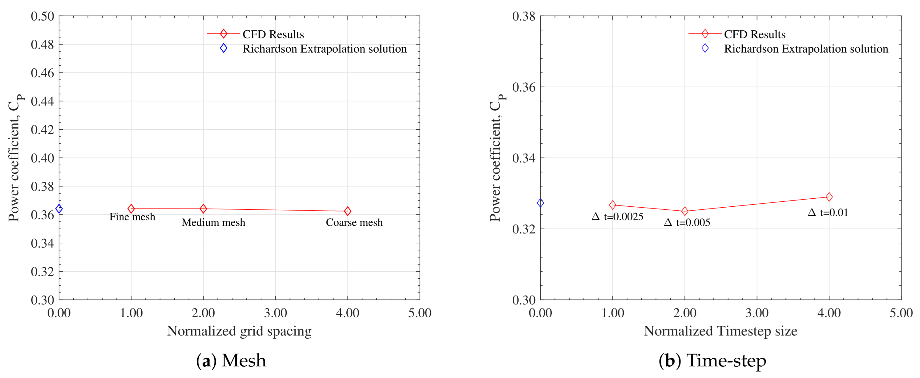
3.1. Numerical Results

Table 4. Experimental treatments.

Run	Blade Length, L (mm)	External Diameter, ${\mathit{D}}_{\mathit{e}}$ (mm)	Blade Inclination Angle, $\mathit{\gamma }$ (°)	Numerical ${\mathit{C}}_{\mathit{p}}$ [-]
1	120	150	45	0.291
2	170	250	60	0.337
3	170	150	30	0.242
4	70	200	45	0.270
5	120	200	60	0.327
6	120	250	45	0.330
7	70	150	60	0.268
8	120	200	30	0.252
9	70	250	30	0.236
10	170	250	30	0.287
11	170	200	45	0.333
12	70	150	30	0.217
13	70	250	60	0.281
14	170	150	60	0.320
15	120	200	45	0.315
16	120	200	45	0.315
17	120	200	45	0.315

shows the maximum numerical power coefficient, $C_p$, for each of the 17 study treatments. Treatment 2, with a $C_p$ value of 0.337, exhibits the highest $C_p$ among all treatments.

From the results in Table 4, it can be inferred that there is no direct relationship between any of the parameters and $C_p$. Increasing or decreasing a parameter does not guarantee, by default, an increase in the power coefficient. Additionally, there are multiple configurations with relatively high $C_p$ values (Treatment 2, Treatment 5, Treatment 6, and Treatment 11), indicating that optimization is a multivariable and complex problem. Given that the $C_p$ values are very close for some treatments, for example, Treatment 2 has a $C_p$ of 0.337 and Treatment 11 has a $C_p$ of 0.333. This suggests that small modifications in the independent factors can have a significant impact on the turbine’s performance.

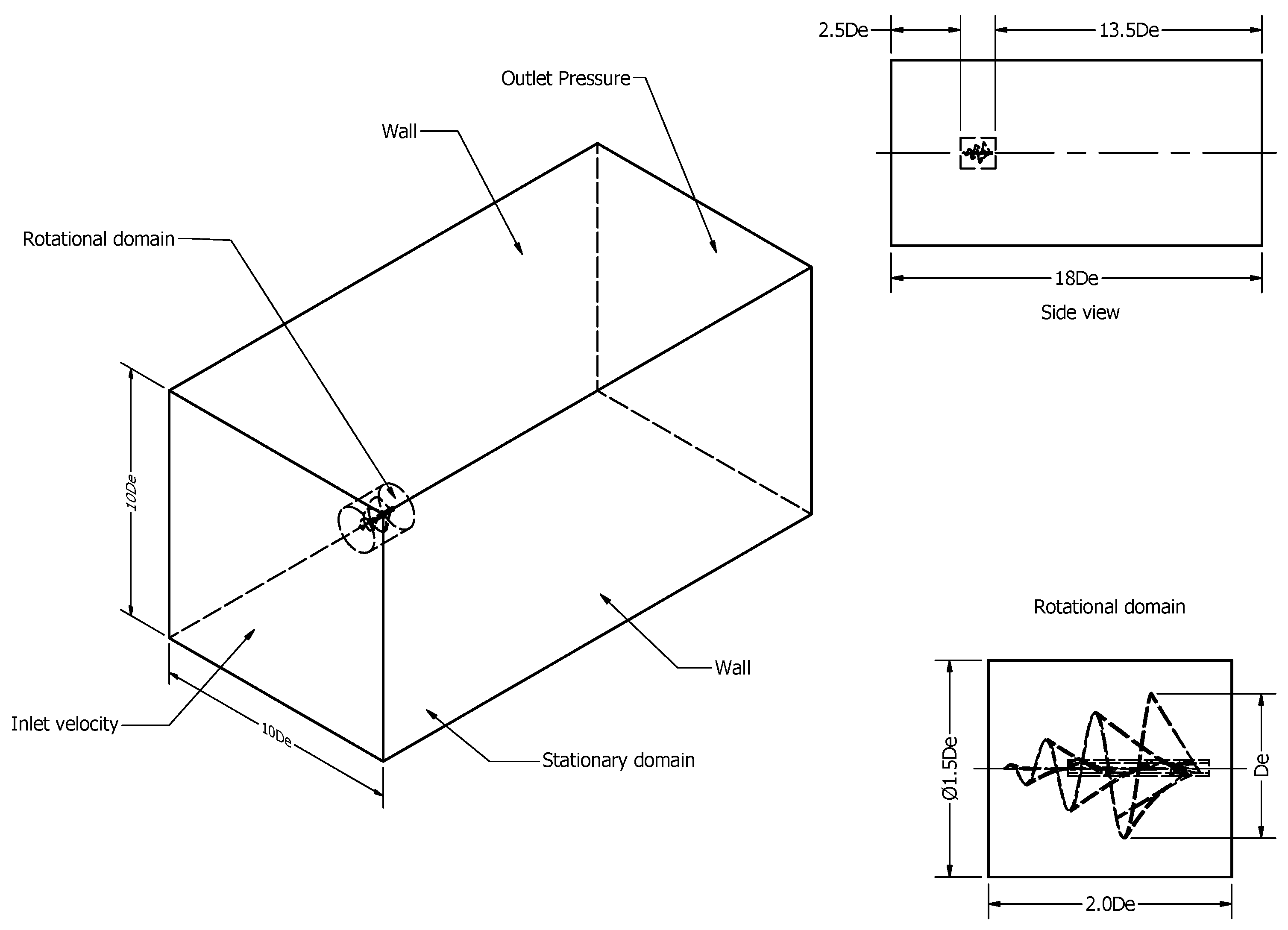
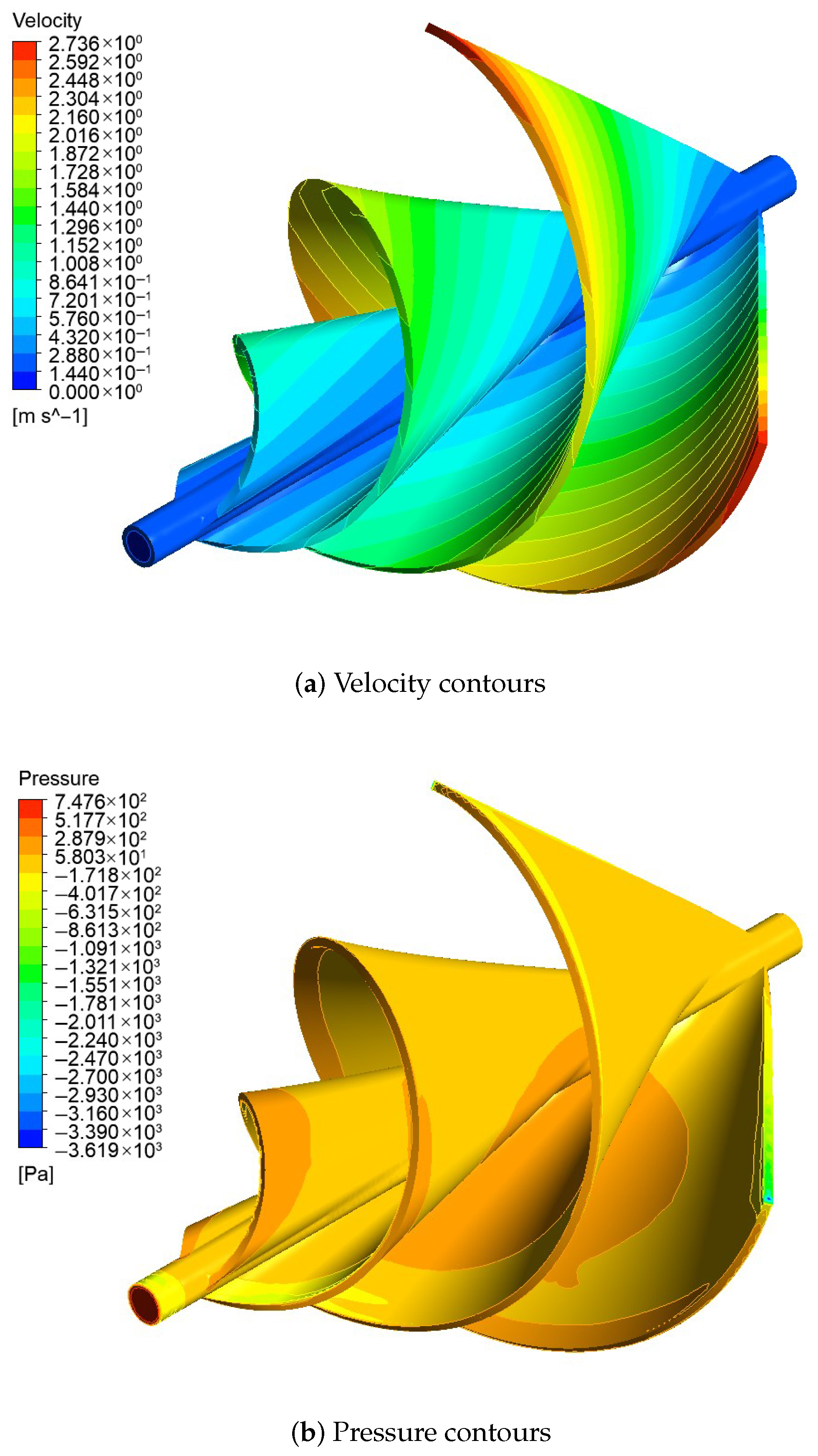
Figure 10 presents the velocity and pressure contours for Treatment 2. In the presented figures, the color spectrum denotes the intensity of the velocity or pressure fields. Warmer tones correspond to greater magnitudes, while cooler tones signify lesser values. Figure 10a reveals that high-velocity regions are concentrated near the blade tips, while low-velocity regions occur in stagnation zones and flow separation regions. Figure 10b demonstrates that the fluid impinging on the rotor blades results in high-pressure regions, whereas regions of low pressure correspond to zones of fluid acceleration.

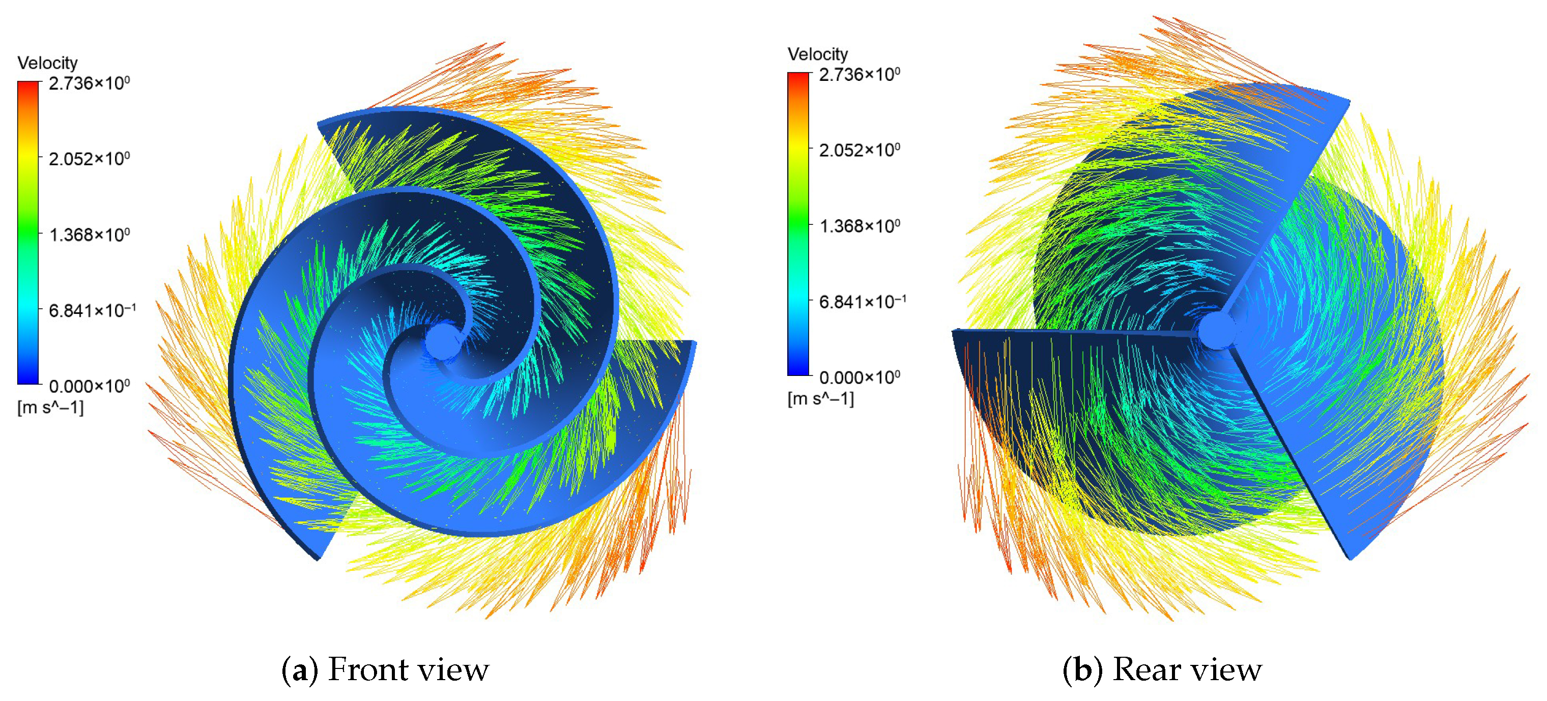
Figure 11 shows the velocity vectors exiting the rotor in the rear and front views. The velocity vectors show the direction and magnitude of the fluid flow as it inlets and exits the rotor. We can observe the formation of a swirling flow pattern, which is characteristic of many types of rotating machinery. The color coding reveals the distribution of velocities across the rotor inlet and exit plane. It can be seen that the velocity is higher near the blade tips and lower near the hub.

Given the complexity of the problem presented in Table 4, a more in-depth statistical analysis will be conducted using the open-source statistical software R 2024.12.0. This analysis aims to identify the optimal combination of factors that maximizes the power coefficient, $C_p$.

3.2. Statistical Analysis

3.2.1. Regression Model Development

A regression model was constructed using $C_p$ from Table 4 and analyzed through ANOVA. This approach allowed for identifying the contribution of each term within the model. To evaluate the model’s effectiveness in accurately reflecting the numerical results, several statistical metrics were considered: the correlation coefficient ($R^2$), the adjusted correlation coefficient ($R_{adj}^2$), and the p-value of the model. Given the potential for nonlinear relationships and the possibility of interactions among the predictors, a second-order regression model was deemed the most appropriate choice for this analysis. This model allows for the inclusion of both linear and quadratic terms, as well as interaction terms, to account for more complex relationships.

Table 5. Results of the analysis of variance.

Term	Sum of Square	Degrees of Freedom	Mean Square	F-Ratio	p-Value
Model		7		40.99	0.0000312
$\gamma$	0.008913	1	0.008913	147.169	0.00000591
L	0.006113	1	0.006113	100.943	0.0000207
$D_e$	0.001758	1	0.001758	29.027	0.001022
${\gamma }^2$	0.001652	1	0.001652	27.27	0.001223
$L^2$	0.003057	1	0.003057	50.469	0.000193
$D_e^2$	0.000453	1	0.000453	7.473	0.029181
$\gamma L$	0.000126	1	0.00126	2.082	0.192225
$\gamma D_e$	0.000146	1	0.000146	2.413	0.164265
$L{D}_e$	0.000124	1	0.000124	2.045	0.195810
Error	0.000424	7	0.000061

shows the results of ANOVA for the second-order model, which examines the relationship between the response variable and the independent variables.

The small p-value (0.0000312) strongly suggests that the overall model is statistically significant, implying its ability to account for a considerable amount of the variation observed in the response variable. The linear components ($\gamma$ and L) and the quadratic components (${\gamma }^2$, $L^2$, and $D_e^2$) exhibit high statistical significance (very small p-values), indicating that both their direct and squared effects play a crucial role in explaining the changes in the response. Conversely, the interaction components ($\gamma L$, $L{D}_e$, and $\gamma D_e$) are not statistically significant (p-value exceeding 0.05), suggesting that the combined effects of these variable pairs do not meaningfully contribute to the model’s explanatory power. The ‘error’ component represents the portion of the response variability that the model does not explain. The small mean squared error suggests a good agreement between the predictions and the actual data. Considering these results, we can infer that the second-order regression model is appropriate for describing the relationship between $C_p$ and the independent variables.

Among the studied factors, the blade inclination angle ($\gamma$) had the most significant influence on $C_p$, with a p-value of 0.00000591. Physically, this strong influence is due to the angle’s critical role in determining how the incoming water flow interacts with the turbine blades. The inclination directly affects the alignment of the blade surfaces relative to the flow direction, which governs the efficiency of momentum transfer from the fluid to the rotor. An optimal angle maximizes the hydrodynamic thrust while minimizing flow separation and energy losses, thereby enhancing the conversion of kinetic energy into mechanical rotation.

The blade length (L), with a p-value of 0.0000207, also exhibits a statistically significant impact on $C_p$. From a physical standpoint, the length of the turbine determines the volume of fluid that interacts with the screw per unit of time. Longer blades increase the surface area available for fluid contact, enabling greater momentum exchange. Additionally, a longer turbine allows for an extended fluid-structure interaction path, enhancing energy capture. However, beyond a certain point, increases in length may lead to structural limitations or frictional losses, highlighting the importance of optimizing this parameter within practical constraints.

The external diameter ($D_e$) showed a statistically significant, albeit comparatively lower, influence on $C_p$, with a p-value of 0.001022. Physically, $D_e$ defines the frontal area through which the turbine intercepts the incoming water flow, directly affecting the amount of kinetic energy available for extraction. A larger diameter increases the swept area, thereby enhancing the theoretical energy capture potential. However, this geometric increase also brings certain trade-offs: a larger $D_e$ leads to greater rotational inertia, which can reduce the responsiveness of the rotor to changes in flow velocity. Additionally, it may result in higher frictional losses due to proximity to channel walls and the generation of unutilized secondary flows. These effects can limit the practical gains in efficiency, underscoring the need to balance energy capture with hydrodynamic and mechanical losses when selecting the optimal diameter.

Beyond the analysis of variance findings detailed in Table 5, the second-order regression model yielded an $R^2$ value of 0.9814. This signifies that the model accounts for roughly 98.14% of the variance in the response. The $R_{adj}^2$, which accounts for the number of predictors in the model, was 0.9574. This suggests strong generalizability of the model to unseen data and confirms the importance of the incorporated variables in elucidating the observed variation. Based on the ANOVA results, Equation (8) represents the final regression model developed. This model was selected as it provided the best fit to the data and was statistically significant.

$$\begin{array}{cc}\hfill C_p=& -0.2285+0.01243\gamma +0.0011443L+0.0009396D_e+0.0000052940\gamma L\hfill \\ \hfill & -0.0000056990\gamma D_e+0.0000015740L{D}_e-0.0001103{\gamma }^2\hfill \\ \hfill & -0.00000501L^2-0.0000015170D_e^2\hfill \end{array}.$$

(8)

3.2.2. Assumption Verification

To validate the second-order regression model, several diagnostic checks are typically performed. Key assumptions to check include linearity, homoscedasticity, and normality of residuals [67,68]. Violation of these assumptions can undermine the model’s reliability and may require adjustments or the use of alternative modeling techniques. Validating a regression model is essential, as it assesses how effectively the model fits the data and predicts new, unseen observations. A thoroughly validated model ensures greater reliability and accuracy in its results [69].

A fundamental assumption in linear regression is that the residuals are normally distributed. To assess this assumption, various statistical tests and graphical methods are employed. Normality tests, such as the Shapiro–Wilk, Jarque–Bera, and Cramer–von Mises tests, provide p-values indicating the likelihood of observing the data if the residuals were truly normally distributed [70,71]. Small p-values suggest a significant departure from normality. Additionally, visual inspection of a histogram of the residuals can reveal skewness or excess kurtosis. A Q–Q plot allows for a comparison of the empirical distribution of the residuals to a theoretical normal distribution; significant deviations from the diagonal line cast doubt on the normality assumption. Non-normal residuals can compromise the validity of statistical inferences based on the model and the accuracy of confidence intervals. Figure 12 shows the Frequency Distribution and Q–Q Plot, while

Table 6. Normality assessment of the response variable.

Normality Test	p-Value
KS limiting form	0.7951
D’Agostino and Pearson test	0.57752
KS Marsaglia method	0.7384
Cramer–von Mises test	0.0992
KS Stephens modification	0.1500
Anderson–Darling test	0.0571
Jarque–Bera test	0.7560

provides the results of the normality tests for the response variable.

The histogram of the residuals, Figure 12a, shows a roughly bell-shaped distribution, which is indicative of a normal distribution. However, there seems to be a slight right skew, suggesting that there might be a few outliers or that the distribution is not perfectly symmetric. The Q–Q plot, Figure 12b, shows that the majority of the points fall approximately along the diagonal line, indicating a reasonable fit to a normal distribution. However, there are some deviations at the tails, particularly in the upper right quadrant, which could suggest slightly heavier tails than a normal distribution. The p-values from the various normality tests, in Table 6, are generally quite high, indicating that it fails to reject the null hypothesis of normality. This means that there is not enough evidence to conclude that the residuals are significantly different from a normal distribution. However, it is worth noting that some of the p-values are closer to the significance level (e.g., 0.05), which could suggest a borderline case. Overall, the evidence suggests that the residuals are reasonably normally distributed.

Before proceeding further with the regression analysis, it must verify the assumption of independent errors. Autocorrelation, or correlation between successive error terms, can lead to biased estimates and unreliable confidence intervals. To test for autocorrelation, it uses the Durbin–Watson test. This test provided a p-value that tells if there is significant evidence of autocorrelation [72,73]. If the p-value is less than the chosen significance level, it concludes that the residuals are not independent, suggesting that it may need to adjust the model. The test produced a p-value of 0.255, suggesting that the independence assumption, meaning there is no self-correlation in the errors, holds true, and we fail to reject it.

To finalize the examination of the regression model’s underlying assumptions, evaluating the assumption of consistent error variance, or homoscedasticity, is crucial. Breaches of this assumption, termed heteroscedasticity, can lead to skewed standard errors and untrustworthy hypothesis tests, potentially undermining the accuracy of the model’s conclusions [74]. The Breusch–Pagan test is a frequently used method for identifying heteroscedasticity. A p-value from this test below the selected significance level suggests the existence of heteroscedasticity, implying that the model might need modifications, such as data transformation or the use of robust standard errors, to guarantee more dependable outcomes. Given a p-value of 0.431, the constant variance assumption is met.

Table 7. Comparison of results.

Experimental Treatments	Numerical ${\mathit{C}}_{\mathit{p}}$ [-]	Predicted ${\mathit{C}}_{\mathit{p}}$ [-]	Residuals [-]
1	0.291	0.298	−0.007032
2	0.337	0.345	−0.008475
3	0.242	0.243	−0.001270
4	0.270	0.278	−0.007355
5	0.327	0.320	0.006737
6	0.330	0.324	0.005952
7	0.268	0.270	−0.001762
8	0.252	0.260	−0.007837
9	0.236	0.237	−0.001063
10	0.287	0.286	0.001132
11	0.333	0.327	0.006272
12	0.217	0.209	0.007845
13	0.281	0.280	0.000643
14	0.320	0.320	0.000435
15	0.315	0.315	−0.000098
16	0.315	0.315	−0.000098
17	0.315	0.315	−0.000098

provides a comparison between the results obtained from simulations and those predicted by the regression model, presenting the residual values.

3.2.3. Determination of the Optimal Point

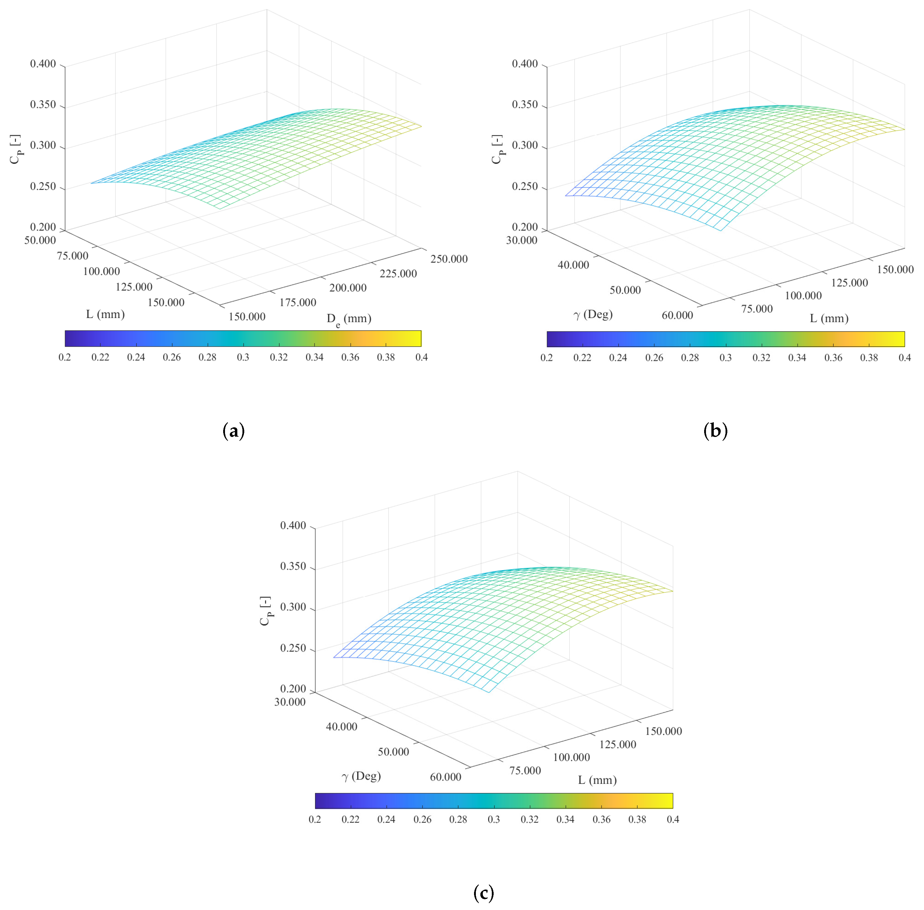
Having developed and validated a second-order regression model, it can now utilize the resulting equation to determine the ideal combination of independent variables that maximizes $C_p$. This is the last step in the response surface methodology optimization process. Statgraphics Centurion XVII software was employed to determine the optimal combination of factor levels. Figure 13 shows the response surface from the optimization process.

Figure 13a illustrates the influence of L and $D_e$ on $C_p$. The surface exhibits a general upward trend as both L and $D_e$ increase, suggesting that higher values of L and $D_e$ tend to yield higher values of $C_p$. The curved nature of the surface indicates a nonlinear relationship between L, $D_e$, and $C_p$, revealing an interaction between these two factors. The effect of varying L on $C_p$ is dependent on the value of $D_e$, and vice versa. Figure 13b displays the impact of L and $\gamma$ on $C_p$. Similar to Figure 13a, an upward trend is observed as both L and $\gamma$ increase. The highest regions of the surface correspond to combinations of L and $\gamma$ that produce the maximum values of $C_p$, whereas the lowest regions correspond to combinations yielding the minimum values of $C_p$. Figure 13c demonstrates a similar behavior to Figure 13a,b, where, in general, increasing values of $D_e$ and $\gamma$ tend to increase the value of $C_p$. There likely exist specific regions within the design space (combinations of L, $D_e$, and $\gamma$) where maximum $C_p$ values are achieved, even if these values do not correspond to the maximum limits for each individual factor. These optimal regions may vary depending on the interactions between the variables and the constraints of the system. The optimization process yielded the following optimal values: $L=168.921$ mm, $D_e=245.645$ mm, and $\gamma =51.341$°. These settings resulted in a maximum $C_p$ value of 0.347. The values obtained do not attain the upper bounds of each independent variable.

Table 8. Experimental treatment and optimal values.

Run	Blade Length, L (mm)	External Diameter, ${\mathit{D}}_{\mathit{e}}$ (mm)	Blade Inclination Angle, $\mathit{\gamma }$ (°)	${\mathit{C}}_{\mathit{p}}$ [-]
Optimal	168.921	245.645	51.341	0.347
2	170	250	60	0.337

presents a comparison of the values for L, $D_e$, and $\gamma$ between the ideal model obtained from the regression model and the model with the highest $C_p$ from the initial treatments, Treatment 2; this is also the treatment where the maximum values for each factor are used.

The optimal point outperforms Treatment 2 by 2.97% in terms of $C_p$, demonstrating that intermediate $\gamma$ values and precise adjustments of L and $D_e$ are crucial for maximizing system performance. This indicates that the regression model effectively identifies factor combinations enhancing system performance.

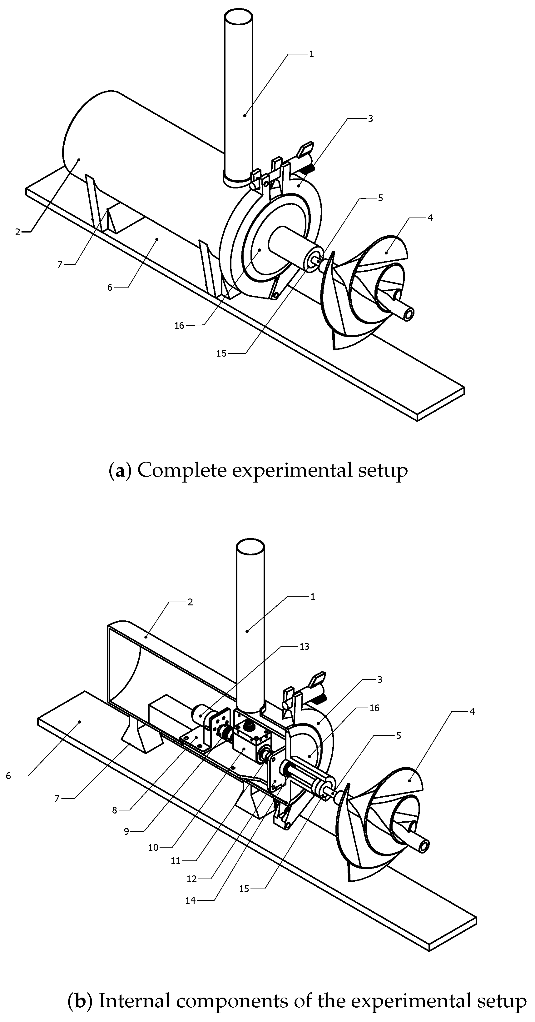
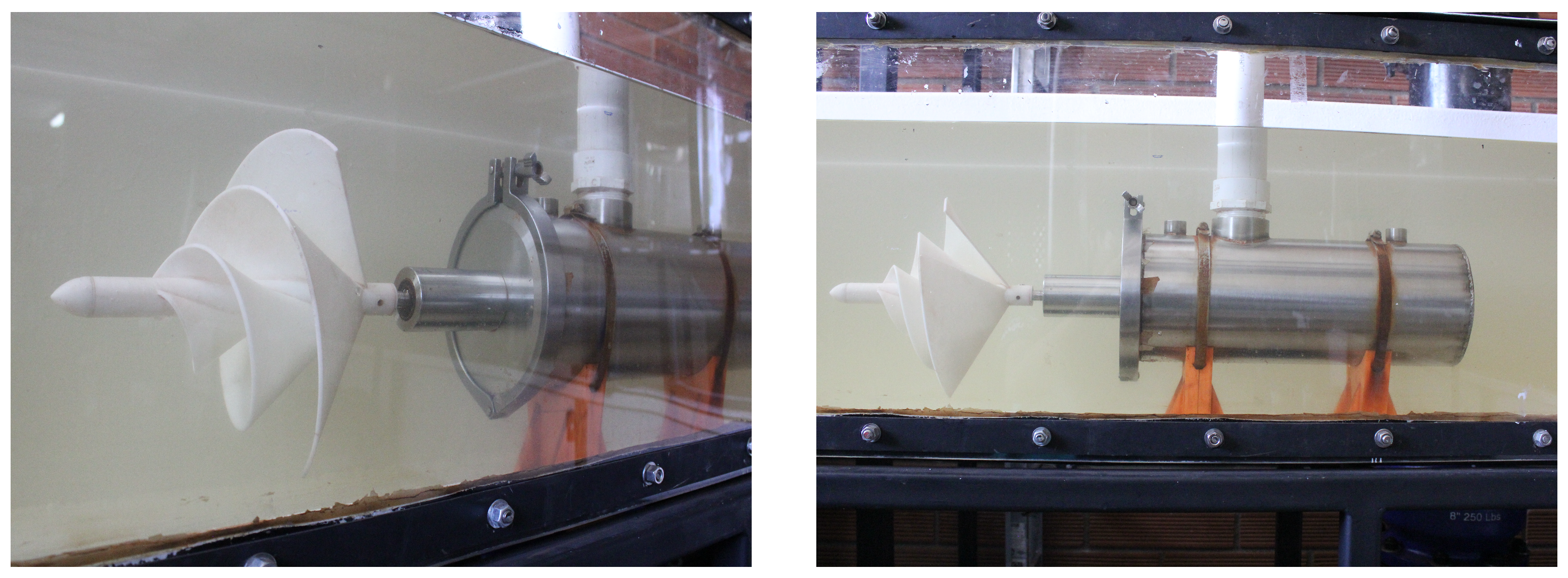
3.3. Experimental Results

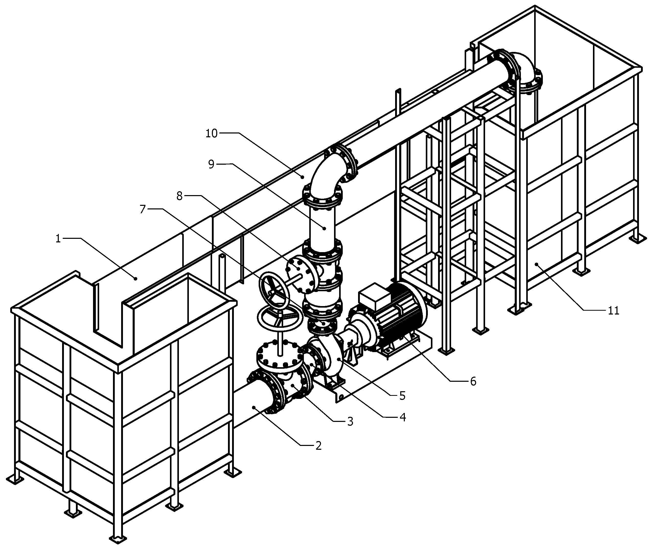
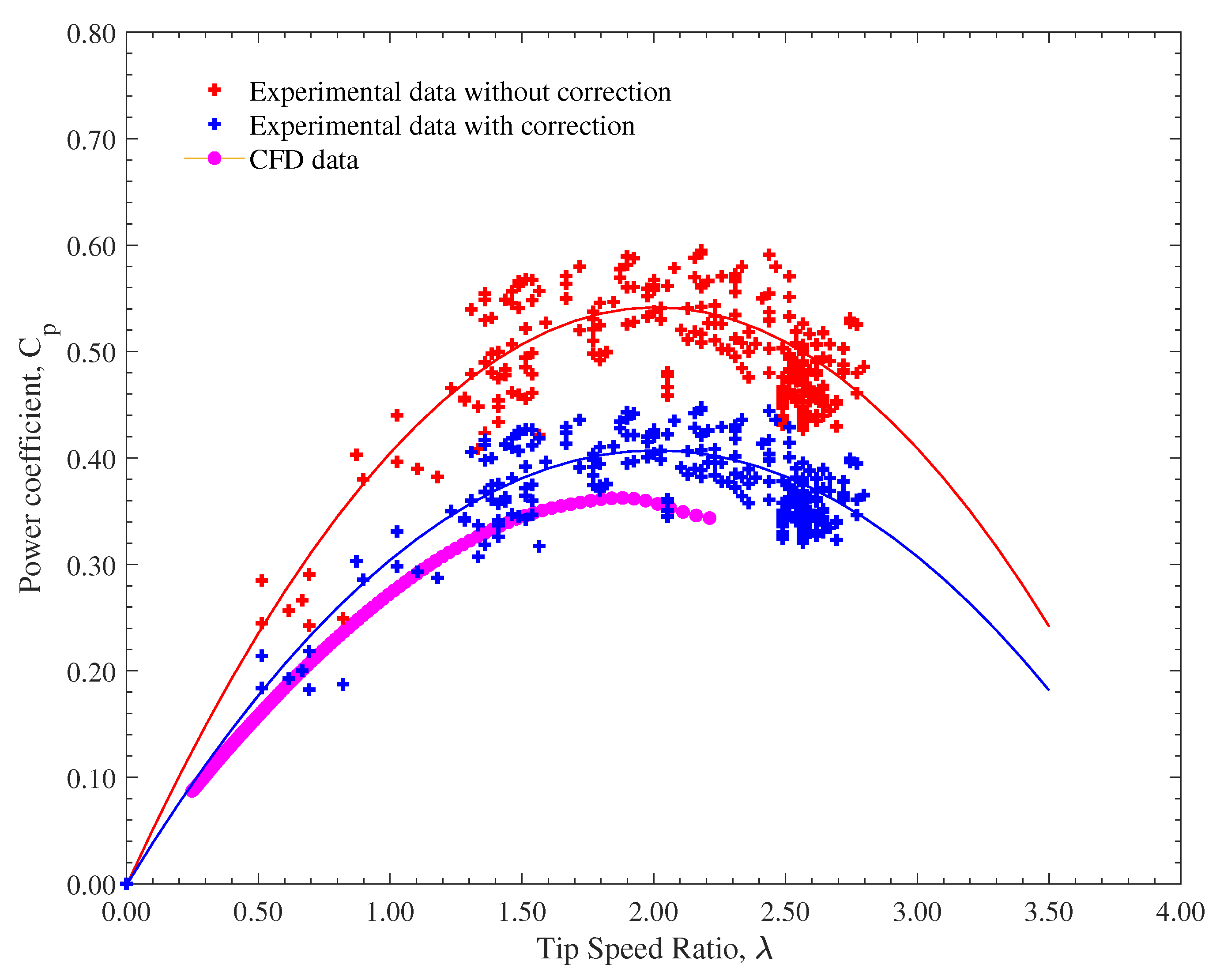
To assess the optimized turbine’s performance, multiple laboratory tests were implemented with a flow velocity of 0.5 m/s in the channel. Figure 14 presents the results obtained from these experiments. The presented Figure shows the relationship between $C_p$ and $TSR$ of the Archimedean spiral turbine.

The red crosses represent raw data obtained directly from the experimental tests (experimental data without correction). The scatter in these points is typical of experimental data due to factors such as measurement noise. The red line represents a second-order polynomial fit to the experimental data. This fit allows for visualization of the overall trend in the data and facilitates the identification of the point of maximum efficiency. The pink data points depict the computational fluid dynamics results corresponding to the optimal treatment.

The characteristic curve of the Archimedean spiral turbine exhibits a typical behavior for hydrokinetic turbines. As $TSR$ rises, $C_p$ initially grows, achieves a peak value, and subsequently declines. The maximum $C_p$ achieved in the experiments was 0.541, which is higher than the value of 0.337 obtained from the optimal treatment. The experimental $TSR$ corresponding to the maximum $C_p$ is 2.12.

The blocking factor ($\beta$) in hydrokinetic turbine experiments refers to the ratio of the turbine’s projected area to the wetted cross-sectional area of the flow channel [28,75,76]. This factor quantifies the obstruction caused by the turbine to the fluid flow, which can significantly influence the turbine’s performance and the accuracy of experimental measurements [77,78]. A higher blocking factor generally leads to increased turbulence and flow distortions, affecting the turbine’s efficiency and power output. To account for the effects of the blocking factor, various correction methods have been proposed [76,78,79,80]. One commonly used approach is the Pope and Harper correction. This method involves adjusting the measured velocity data to compensate for the blockage effects [28,79]. The correction factor is calculated based on the blockage ratio, which is the ratio of the turbine’s projected area to the free-stream flow area. By applying this correction factor, it is possible to obtain more accurate estimates of the turbine’s performance in an unobstructed flow.

The Pope and Harper method employs a correction factor, $\alpha$, to account for the blockage effect on velocity measurements. This factor is determined by the equation $\alpha =(1+\beta /4)$, where $\beta$ is the ratio of the blocked area to the total flow area [76,78]. In this specific case, the turbine has an area of 0.047 m², and the wetted area of the channel is 0.118 m², corresponding a blocking factor of 0.398. This means that the turbine blocks approximately 40% of the flow.

Given a $\beta$ value of 0.398, the blockage factor is determined to be 1.099. By applying the Pope and Harper correction, the original measured velocity of 0.5 m/s is multiplied by the correction factor $\alpha$, yielding an adjusted velocity of 0.5498 m/s. This velocity adjustment leads to an increase in the available power in the flow from 2.96 W to 3.93 W. However, it is important to note that this apparent increase in power is likely due to the overestimation of the actual flow velocity caused by the blockage effect. Consequently, the turbine efficiency is underestimated when using the uncorrected velocity data. Figure 14 shows the experimental data, corrected using the Pope and Harper method, represented by blue crosses. The blue line represents the polynomial fit to the corrected data.

The maximum experimental $C_p$ achieved was 0.407, which is approximately 14% higher than the numerical value of 0.347 obtained from the regression model. While this discrepancy may be attributed in part to inherent limitations in the regression model, which has an $R_{adj}^2$ of 0.9574, other factors also contribute to the observed difference between experimental and numerical results. For instance, the CFD simulations were conducted at a constant inlet velocity of 1.2 m/s, whereas the experimental tests were performed at a lower flow speed of 0.5 m/s due to constraints in the test channel. This difference in flow velocity can significantly affect the Reynolds number and, consequently, the flow behavior around the blades, influencing turbine performance.

Moreover, the CFD model assumes idealized boundary conditions—such as uniform inlet flow and the absence of disturbances—which differ from real experimental conditions where flow may be slightly non-uniform and affected by minor turbulence, wall effects, or setup vibrations. On the experimental side, measurement uncertainty, sensor precision, and mechanical losses (e.g., friction in the shaft or support structure) may also influence the recorded $C_p$. Despite these factors, the discrepancy between the two values is substantially smaller than the overestimated $C_p$ of 0.541 obtained when the Pope and Harper correction is not applied, reinforcing the validity of the chosen correction method and optimization strategy. The experimental $TSR$ corresponding to the maximum $C_p$ is 2.12, representing the turbine’s optimal operating point for converting fluid kinetic energy into mechanical work.

Although the present study identified an optimal configuration based on numerical simulations and validated it experimentally under controlled laboratory conditions, the performance of the ASHT may differ when deployed in natural rivers or tidal streams. For example, highly turbulent or unsteady flows may affect the flow attachment along the blades and, consequently, the power coefficient ($C_p$). Similarly, lower or fluctuating flow velocities may reduce energy capture efficiency.

To address these limitations and enhance generalizability, future work should focus on testing the optimized ASHT in various natural water bodies. Field experiments across different hydrodynamic conditions will be essential to evaluate long-term reliability and performance. Moreover, incorporating site-specific parameters into future optimization frameworks, such as local velocity profiles, turbulence spectra, and environmental constraints, can help tailor turbine designs to particular deployment sites.

4. Conclusions

This study successfully employed a numerical optimization technique to enhance the performance of an Archimedes spiral hydrokinetic turbine (ASHT). By systematically varying key design parameters (blade length L, blade inclinationangle $\gamma$, and external diameter $D_e$) using a central composite design (CCD) approach, the optimal configuration for maximizing the power coefficient ($C_p$) was identified.

The numerical simulations demonstrated that the optimal design yielded a maximum $C_p$ of 0.337 for $L=168.921$ mm, $\gamma =51.341$° and $D_e=245.645$ mm. Subsequent experimental validation confirmed the accuracy of the numerical predictions, with a slightly higher $C_p$ of 0.407 achieved experimentally. This discrepancy may be attributed to factors such as variations in experimental conditions or limitations in the numerical model. The optimization process revealed that the optimal design does not necessarily correspond to the maximum values of each design parameter. Instead, a balance between these parameters is crucial for achieving optimal performance.

To further refine the accuracy of numerical predictions, future research should incorporate more advanced turbulence models and consider unsteady flow effects. Additionally, a comprehensive experimental campaign with a wider range of operating conditions and flow velocities can provide valuable insights into the turbine’s performance and limitations.

Furthermore, investigating the impact of different materials on the turbine’s performance and durability, as well as optimizing the structural design to minimize weight and maximize strength, is crucial. Multi-objective optimization, considering additional performance metrics such as efficiency and structural integrity, can lead to more balanced designs. Ultimately, deploying the optimized ASHT in real-world river environments will be essential to assess its long-term performance and reliability. By addressing these areas, future research can further advance the development and deployment of ASHTs as a sustainable and efficient source of renewable energy.

Finally, evaluating the scalability of the optimized design is essential to facilitate its transition from laboratory-scale prototypes to full-scale, real-world applications. Scaling up the ASHT must account for changes in Reynolds number, structural loading, and fabrication constraints that could influence hydrodynamic performance and mechanical integrity. Future studies should investigate the performance of geometrically scaled models under realistic flow conditions to ensure that the design principles remain effective across various sizes and deployment scenarios.