Dynamical Modeling and Active Vibration Control Analysis of a Double-Layer Cylindrical Thin Shell with Active Actuators

Abstract

The application of double-layer shell structure is very common in some situations that require complex loads and vibrations, such as key components such as the shell and wings of aerospace engines, and the shell of underwater vehicles. Many authors have conducted research on the vibration and acoustic radiation characteristics of double-layer cylindrical shells. By adding reinforcement and ribs between the double-layer cylindrical shells and optimizing structural design, passive vibration control techniques can effectively solve high frequency vibration problems, but the impact on mid to low frequency vibrations is still limited. Therefore, this article conducts theoretical research on a novel active vibration control method that inserts an active actuator between a double-layer cylindrical shell to achieve better mid low frequency vibration control effects. Firstly, the substructure admittance method is applied to analytically and dynamically model a double-layer cylindrical thin shell structure with active support, and the vibration power flow of the system is theoretically derived to evaluate the vibration reduction effect. Then, numerical simulation analysis was conducted on the influence of different configurations of six feedback control parameters, time delays, and other factors on the vibration power flow. Finally, based on the image, the conclusion is drawn that all six feedback control parameters can improve the vibration control effect of the coupled system to a certain extent, but not every feedback control parameter has a prominent effect, and the effective range of some parameters is relatively narrow.

1. Introduction

The advantages of cylindrical shell structure are light weight, high load-bearing capacity, and low material usage, making it widely used in engineering applications. For example, silos, towers, and chimneys in civil engineering, launch vehicles in the aerospace industry, military submarines [1,2], common storage tanks and gas pipelines, as well as many specific structures in energy and power engineering such as steam turbines and gas turbines all adopt cylindrical shell-like shapes.

In order to ensure the excellent performance of cylindrical shells in engineering and improve the safety and reliability of related structures, studying their mechanical behavior, structural strength, vibration characteristics, and control has been an important topic for a long time. For example, the stability of cylindrical thin shells under different loads such as axial pressure and local pressure [3]; the influence of special structures, coatings, pore distribution, surface cracks, etc. on the vibration modes of cylindrical thin shells [4,5,6]; the preparation and vibration characteristics of advanced composite cylindrical shells [7]; the influence of temperature [8]; etc.

The double-layer cylindrical thin shell can be regarded as a complex structural form of cylindrical shell. Computational analysis shows that the strength and load-bearing capacity of double-layer reinforced cylindrical shells with different structural forms are superior to single-layer cylindrical shells under the same conditions [9]. When the thickness of the double-layer and single-layer cylindrical shells is the same, the double-layer cylindrical shell can better meet the requirements of strength and bearing capacity. Its critical pressure has a significant advantage, and under the same pressure and aspect ratio, the weight of the double-layer reinforced cylindrical shell is always lower than that of the single-layer reinforced cylindrical shell, which means less material is used and stronger manufacturing feasibility [10,11]. Therefore, in some environments that require complex loads and vibrations, the application of double-layer shell structures is more common, such as key components such as the outer shell and wings of aerospace engines, and the outer shell of underwater vehicles [12].

Many authors have conducted research on the vibration and acoustic radiation characteristics of double-layer cylindrical shells. By adopting optimized structural design and effective vibration control techniques, the performance of double-layer cylindrical thin shells can be significantly improved. One common method is to arrange passive supports [13], such as reinforcement and ribs, for passive vibration control. At the same time, the influence of different parameter characteristics on the critical shells can be investigated, providing technical support for the design and calculation of ring ribbed cylindrical shells [14]. The study in reference [15] shows that for ribbed cylindrical thin shells, using non-periodic arrangement of rib spacing of changing the position of ribs has little effect on low frequency vibration. In addition, methods such as viscoelastic damping materials [16] and dynamic vibration absorber [17] can also be used to reduce vibration, which can effectively solve high frequency vibration problems. However, their impact on mid to low frequency vibration is still limited.

According to relevant research trends, active vibration control is an effective means for low frequency vibration problems [18], among which piezoelectric sensors and actuators are commonly arranged on the shell structure, combined with intelligent control algorithms, to monitor and adjust the vibration response of the structure in real time: Reference [19] conducted theoretical and experimental research on piezoelectric energy harvesters with cylindrical shell structures, and found that selecting appropriate parameters for the controlled can reduce the amplitude of structural vibration and shorten the steady-state response time. For the optimization problem of actuator position in active vibration control, the study in reference shows [20] that using genetic algorithm to optimize the placement position of thickness actuators can achieve better vibration control effects. The disadvantage of the active vibration control method based on piezoelectric intelligent structures mentioned above is that it is generally limited to lightweight structure; in addition, piezoelectric materials are brittle, and when combined with an elastic matrix to form a multi-layer structure, their interfaces can cause stress concentration, which can easily lead to failures such as cracks and delamination [21].

Due to the complexity of the structure, theoretical research on vibration control of double-layer cylindrical shells also involves complex dynamic modeling. Reference [22] focuses on the design and vibration performance analysis of composite multi-layer cylindrical shell structures, discussing the complexity of solving shell vibration and sound radiation problems, as well as the development process, research status, and applicable scope of shell theory. Reference [23] proposes a method for establishing a vibration model of a double-layer cylindrical thin shell using neural networks. Comparison with finite element models and experimental data shows that although the model has higher accuracy, it usually requires relatively large experimental data. References [24,25] proposed a method of modeling uniformly mass cylindrical shells and annular plates as spectral elements, which can accurately and quickly calculate the natural frequencies and vibration responses of ribbed cylindrical shells under any boundary conditions. Generally speaking, digital modeling methods such as finite element method can better describe irregular detailed structures, but the modeling and computational costs are relatively high; For the theoretical research of mechanism, analytical modeling methods have high analysis efficiency and low modeling costs, making them a more practical approach.

This article presents a theoretical study on a novel active vibration control method that inserts an active actuator between a double-layer cylindrical thin shell. This method can provide greater control force than previous active vibration control based on piezoelectric intelligent structures, thereby achieving better mid to low frequency vibration control effects. Based on the dynamic modeling of the double-layer cylindrical thin shell and the supporting structure between the two shells, and based on the evaluation index of vibration power flow, this paper conducts numerical simulation analysis on the influence of different configurations and time delays of six feedback control parameters (absolute displacement, velocity, acceleration feedback control, relative displacement, velocity, acceleration feedback control), and summarizes the effectiveness and scope of the above active control methods.

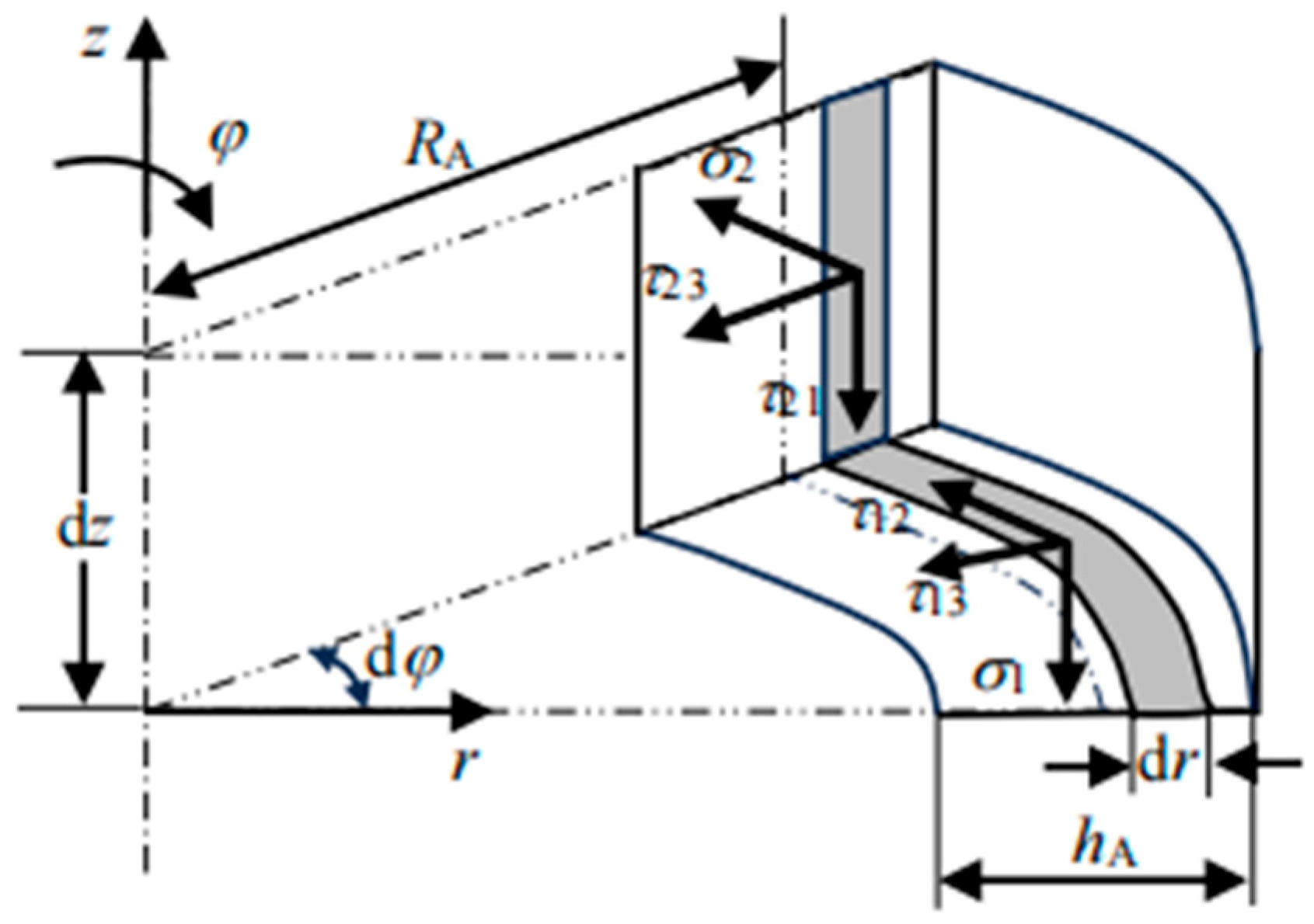
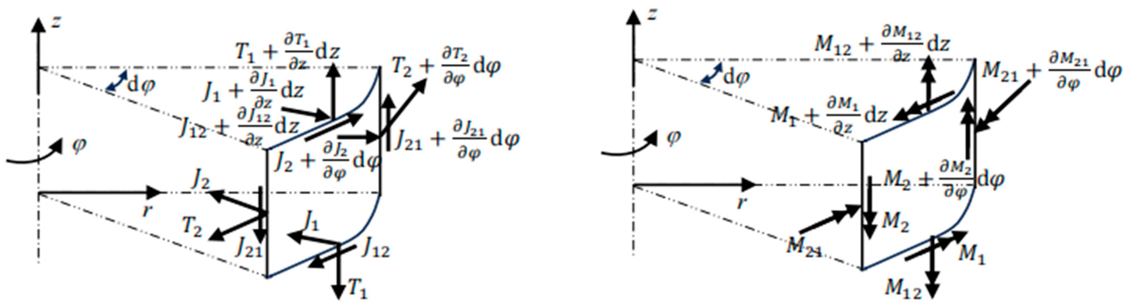
2. Dynamic Modeling of Double-Layer Cylindrical Thin Shell

Figure 1 shows the double-layer cylindrical thin shell model discussed in this article, which includes two coaxial and same height cylindrical thin shells (inner shell A with a center radius of $R_{\mathrm{A}}$ and a thickness of $h_{\mathrm{A}}$, and outer shell B with a center radius of $R_{\mathrm{B}}$ and a thickness of $h_{\mathrm{B}}$). Several supporting structures (assumed to be N in the figure) are inserted between A and B to enhances their lateral load-bearing capacity. The system is placed in a cylindrical coordinate system, with the coordinate origin located at the center of the bottom surface of the cylindrical shell and the z-axis along the axis direction.

In Figure 1, $f_{\mathrm{e}}(z,\phi ,r,t)$ represents vibration excitation acting on the inner shell A, and $(z,\phi ,r)$ represents cylindrical coordinates; $F_{\mathrm{I}1},F_{\mathrm{I}2},\dots ,F_{\mathrm{I}N}$ represent the dynamic forces exerted by each support on the A and B shells, ignoring the mass of each support. Therefore, their forces on the A and B shells are equal in magnitude and opposite in direction. Active vibration control refers to the use of active actuators between the inner and outer shells or the parallel connection of active actuators and passive supports, and the use of active actuators to output active control force to suppress the vibration of the system.

The following conducts admittance analysis on two cylindrical thin shells and their three subsystems with intermediate support.

2.1. Admittance Analysis of Cylindrical Thin Shell Subsystems

In engineering, equivalent concentrated excitation is often used based on Saint David’s principle [26] to simplify calculation and analysis. A concentrated harmonic excitation force is applied at point $A_{\mathrm{e}}(z_{\mathrm{e}},{\phi }_{\mathrm{e}})$ on shell A

$$\overrightarrow{F_{\mathrm{e}}}=F_{\mathrm{e}}[\mathrm{c}\mathrm{o}\mathrm{s}{\psi }_{\mathrm{e}1}·\overrightarrow{{\mathrm{e}}_1}+\mathrm{c}\mathrm{o}\mathrm{s}{\psi }_{\mathrm{e}2}·\overrightarrow{{\mathrm{e}}_2}({\phi }_{\mathrm{e}})+\mathrm{c}\mathrm{o}\mathrm{s}{\psi }_{\mathrm{e}3}·\overrightarrow{{\mathrm{e}}_3}({\phi }_{\mathrm{e}})]·\delta (z-z_{\mathrm{e}})·\delta (\phi -{\phi }_{\mathrm{e}})·\mathrm{e}\mathrm{x}\mathrm{p}(\mathrm{j}\omega t)$$

(1)

In the formula, $F_{\mathrm{e}}$ is the amplitude of the excitation force; $\overrightarrow{{\mathrm{e}}_1},\overrightarrow{{\mathrm{e}}_2}({\phi }_{\mathrm{e}})$, and $\overrightarrow{{\mathrm{e}}_3}({\phi }_{\mathrm{e}})$ respectively represent the unit vectors along the longitudinal ($z$-direction), circumferential ($\phi$-direction), and radial ($r$-direction) directions of the cylindrical coordinate system at point $A_{\mathrm{e}}(z_{\mathrm{e}},{\phi }_{\mathrm{e}})$. The direction of $\overrightarrow{{\mathrm{e}}_1}$ is fixed (pointing in the positive direction of the coordinate axis), while the directions of $\overrightarrow{{\mathrm{e}}_2}({\phi }_{\mathrm{e}})$ and $\overrightarrow{{\mathrm{e}}_3}({\phi }_{\mathrm{e}})$ change with the variation of the coordinate value ${\phi }_{\mathrm{e}}$;${\psi }_{\mathrm{e}1},{\psi }_{\mathrm{e}2}$, and ${\psi }_{\mathrm{e}3}$ are the angles between $\overrightarrow{F_{\mathrm{e}}}$ and $\overrightarrow{{\mathrm{e}}_1},\overrightarrow{{\mathrm{e}}_2}({\phi }_{\mathrm{e}}),\overrightarrow{{\mathrm{e}}_3}({\phi }_{\mathrm{e}})$, respectively.

If $u_{\mathrm{A}},v_{\mathrm{A}},w_{\mathrm{A}}$ represent the displacement of the cylindrical thin shell along the three directions, then the vibration differential equation of shell A is

$$\left\{\begin{array}{c}({\displaystyle \frac{{\partial }^2}{\partial z^2}}+{\displaystyle \frac{1-{\mu }_{\mathrm{A}}}{2{R_{\mathrm{A}}}^2}}{\displaystyle \frac{{\partial }^2}{\partial {\phi }^2}})u_{\mathrm{A}}+{\displaystyle \frac{1+{\mu }_{\mathrm{A}}}{2R_{\mathrm{A}}}}{\displaystyle \frac{{\partial }^2{v}_{\mathrm{A}}}{\partial z\partial \phi }}+{\displaystyle \frac{{\mu }_{\mathrm{A}}}{R_{\mathrm{A}}}}{\displaystyle \frac{\partial w_{\mathrm{A}}}{\partial z}}={\displaystyle \frac{1-{{\mu }_{\mathrm{A}}}^2}{E_{\mathrm{A}}{h}_{\mathrm{A}}}}({\rho }_{\mathrm{A}}{h}_{\mathrm{A}}{\displaystyle \frac{{\partial }^2{u}_{\mathrm{A}}}{\partial t^2}}-F_{\mathrm{e}}cos{\psi }_{\mathrm{e}1}·\delta (z-z_{\mathrm{e}})·\delta (\phi -{\phi }_{\mathrm{e}}))\\ {\displaystyle \frac{1+{\mu }_{\mathrm{A}}}{2R_{\mathrm{A}}}}{\displaystyle \frac{{\partial }^2{u}_{\mathrm{A}}}{\partial z\partial \phi }}+({\displaystyle \frac{1-{\mu }_{\mathrm{A}}}{2}}{\displaystyle \frac{{\partial }^2}{\partial z^2}}+{\displaystyle \frac{1}{{R_{\mathrm{A}}}^2}}{\displaystyle \frac{{\partial }^2}{\partial {\phi }^2}})v_{\mathrm{A}}+{\displaystyle \frac{1}{{R_{\mathrm{A}}}^2}}{\displaystyle \frac{\partial w_{\mathrm{A}}}{\partial \phi }}={\displaystyle \frac{1-{{\mu }_{\mathrm{A}}}^2}{E_{\mathrm{A}}{h}_{\mathrm{A}}}}({\rho }_{\mathrm{A}}{h}_{\mathrm{A}}{\displaystyle \frac{{\partial }^2{v}_{\mathrm{A}}}{\partial t^2}}-F_{\mathrm{e}}cos{\psi }_{\mathrm{e}2}·\delta (z-z_{\mathrm{e}})·\delta (\phi -{\phi }_{\mathrm{e}}))\\ -{\displaystyle \frac{{\mu }_{\mathrm{A}}}{R_{\mathrm{A}}}}{\displaystyle \frac{\partial u_{\mathrm{A}}}{\partial z}}-{\displaystyle \frac{1}{{R_{\mathrm{A}}}^2}}{\displaystyle \frac{\partial v_{\mathrm{A}}}{\partial \phi }}-({\displaystyle \frac{1}{{R_{\mathrm{A}}}^2}}+{\displaystyle \frac{{h_{\mathrm{A}}}^2}{12}}{\nabla }^4)w_{\mathrm{A}}={\displaystyle \frac{1-{{\mu }_{\mathrm{A}}}^2}{E_{\mathrm{A}}{h}_{\mathrm{A}}}}({\rho }_{\mathrm{A}}{h}_{\mathrm{A}}{\displaystyle \frac{{\partial }^2{w}_{\mathrm{A}}}{\partial t^2}}-F_{\mathrm{e}}cos{\psi }_{\mathrm{e}3}·\delta (z-z_{\mathrm{e}})·\delta (\phi -{\phi }_{\mathrm{e}}))\end{array}\right.$$

(2)

In the formula, ${\nabla }^4={\displaystyle \frac{{\partial }^4}{\partial z^4}}+{\displaystyle \frac{1}{{R_{\mathrm{A}}}^2}}{\displaystyle \frac{{\partial }^4}{\partial z^2\partial {\phi }^2}}+{\displaystyle \frac{1}{{R_{\mathrm{A}}}^4}}{\displaystyle \frac{{\partial }^4}{\partial {\phi }^4}}$; ${\rho }_{\mathrm{A}},{\mu }_{\mathrm{A}}, E_{\mathrm{A}}$ are the density, Poisson’s ratio, and elastic modulus of the cylindrical thin shell. The specific origin of Formula (2) can be found in the Appendix A.

The solution of Equation (2) has the following superposition form of vibration modes:

$$\left\{\begin{array}{c}{\mathrm{u}}_{\mathrm{A}}(\mathrm{z},\mathrm{\phi },\mathrm{t})={\sum }_{\mathrm{m},\mathrm{n}=0}^{\mathrm{\infty }}{\mathrm{U}}_{\mathrm{A}\mathrm{m}\mathrm{n}}(\mathrm{z},\mathrm{\phi })·{\mathrm{q}}_{\mathrm{m}\mathrm{n}}(\mathrm{t})\\ {\mathrm{v}}_{\mathrm{A}}(\mathrm{z},\mathrm{\phi },\mathrm{t})={\sum }_{\mathrm{m},\mathrm{n}=0}^{\mathrm{\infty }}{\mathrm{V}}_{\mathrm{A}\mathrm{m}\mathrm{n}}(\mathrm{z},\mathrm{\phi })·{\mathrm{q}}_{\mathrm{m}\mathrm{n}}(\mathrm{t})\\ {\mathrm{w}}_{\mathrm{A}}(\mathrm{z},\mathrm{\phi },\mathrm{t})={\sum }_{\mathrm{m},\mathrm{n}=0}^{\mathrm{\infty }}{\mathrm{W}}_{\mathrm{A}\mathrm{m}\mathrm{n}}(\mathrm{z},\mathrm{\phi })·{\mathrm{q}}_{\mathrm{m}\mathrm{n}}(\mathrm{t})\end{array}\right.$$

(3)

In the formula, $q_{mn}(t)$ is the modal influence factor; $U_{\mathrm{A}mn},V_{\mathrm{A}mn},W_{\mathrm{A}mn}$ are modal functions, which have the following orthogonal properties

$${{\rho }_{\mathrm{A}}{h}_{\mathrm{A}}R}_{\mathrm{A}}{\int }_0^L{\int }_0^{2\pi }(U_{\mathrm{A}ij}{U}_{\mathrm{A}mn}+V_{\mathrm{A}ij}{V}_{\mathrm{A}mn}+W_{\mathrm{A}ij}{W}_{\mathrm{A}mn})\mathrm{d}z\mathrm{d}\phi =\left\{\begin{array}{c}{M}_{\mathrm{A}ij} (i=m \mathrm{and} j=n)\\ 0 (i\ne m or j\ne n)\end{array}\right.$$

(4)

In the formula, $M_{\mathrm{A}ij}$ is modal mass, $i,j,m,n\in N_{+}$; $\mathrm{L}$ is the length of a cylindrical thin shell.

Substituting Equation (3) into Equation (2) and based on the orthogonality of the mode function in Equation (4), the modal coordinate equation can be obtained

$${\ddot{q}}_{ij}+{\omega }_{\mathrm{A}ij}^2{q}_{ij}={\displaystyle \frac{F_{\mathrm{e}}·\mathrm{e}\mathrm{x}\mathrm{p}(\mathrm{j}\omega t)}{M_{\mathrm{A}ij}}}[U_{\mathrm{A}ij}(z_{\mathrm{e}},{\phi }_{\mathrm{e}})·\mathrm{c}\mathrm{o}\mathrm{s}{\psi }_{\mathrm{e}1}+V_{\mathrm{A}ij}(z_{\mathrm{e}},{\phi }_{\mathrm{e}})·\mathrm{c}\mathrm{o}\mathrm{s}{\psi }_{\mathrm{e}2}+W_{\mathrm{A}ij}(z_{\mathrm{e}},{\phi }_{\mathrm{e}})·\mathrm{c}\mathrm{o}\mathrm{s}{\psi }_{\mathrm{e}3}]$$

(5)

In the formula, ${\omega }_{\mathrm{A}ij}$ is the natural frequency of each order, $i,j\in N_{+}$.

Note that under harmonic excitation, ${\ddot{q}}_{mn}=-{\omega }^2{q}_{mn}$. According to Equations (3) and (5), the vibration displacement response at any point on the surface of a cylindrical thin shell can be obtained as

$$\begin{array}{c}\overrightarrow{y_{\mathrm{A}}}=u_{\mathrm{A}}·\overrightarrow{{\mathrm{e}}_1}+v_{\mathrm{A}}·\overrightarrow{{\mathrm{e}}_2}+w_{\mathrm{A}}·\overrightarrow{{\mathrm{e}}_3}=\\ {\sum }_{m,n=0}^{\mathrm{\infty }}[{\displaystyle \frac{U_{\mathrm{A}mn}(z_{\mathrm{e}},{\phi }_{\mathrm{e}})U_{\mathrm{A}\mathrm{m}\mathrm{n}}(z,\phi )}{M_{\mathrm{A}mn}({\omega }_{\mathrm{A}mn}^2-{\omega }^2)}}\overrightarrow{{\mathrm{e}}_1}+{\displaystyle \frac{U_{\mathrm{A}mn}(z_{\mathrm{e}},{\phi }_{\mathrm{e}})V_{\mathrm{A}mn}(z,\phi )}{M_{\mathrm{A}mn}({\omega }_{\mathrm{A}mn}^2-{\omega }^2)}}\overrightarrow{{\mathrm{e}}_2}+{\displaystyle \frac{U_{\mathrm{A}mn}(z_{\mathrm{e}},{\phi }_{\mathrm{e}})W_{\mathrm{A}mn}(z,\phi )}{M_{\mathrm{A}mn}({\omega }_{\mathrm{A}mn}^2-{\omega }^2)}}\overrightarrow{{\mathrm{e}}_3}]F_{\mathrm{e}}\mathrm{c}\mathrm{o}\mathrm{s}{\psi }_{\mathrm{e}1}\mathrm{e}\mathrm{x}\mathrm{p}(\mathrm{j}\omega t)+\\ {\sum }_{m,n=0}^{\mathrm{\infty }}[{\displaystyle \frac{V_{\mathrm{A}mn}(z_{\mathrm{e}},{\phi }_{\mathrm{e}})U_{\mathrm{A}mn}(z,\phi )}{M_{\mathrm{A}mn}({\omega }_{\mathrm{A}mn}^2-{\omega }^2)}}\overrightarrow{{\mathrm{e}}_1}+{\displaystyle \frac{V_{\mathrm{A}mn}(z_{\mathrm{e}},{\phi }_{\mathrm{e}})V_{\mathrm{A}mn}(z,\phi )}{M_{\mathrm{A}mn}({\omega }_{\mathrm{A}mn}^2-{\omega }^2)}}\overrightarrow{{\mathrm{e}}_2}+{\displaystyle \frac{V_{\mathrm{A}mn}(z_{\mathrm{e}},{\phi }_{\mathrm{e}})W_{\mathrm{A}mn}(z,\phi )}{M_{\mathrm{A}mn}({\omega }_{\mathrm{A}mn}^2-{\omega }^2)}}\overrightarrow{{\mathrm{e}}_3}]F_{\mathrm{e}}\mathrm{c}\mathrm{o}\mathrm{s}{\psi }_{\mathrm{e}2}\mathrm{e}\mathrm{x}\mathrm{p}(\mathrm{j}\omega t)+\\ {\sum }_{m,n=0}^{\mathrm{\infty }}[{\displaystyle \frac{W_{\mathrm{A}mn}(z_{\mathrm{e}},{\phi }_{\mathrm{e}})U_{\mathrm{A}mn}(z,\phi )}{M_{\mathrm{A}mn}({\omega }_{\mathrm{A}mn}^2-{\omega }^2)}}\overrightarrow{{\mathrm{e}}_1}+{\displaystyle \frac{W_{\mathrm{A}mn}(z_{\mathrm{e}},{\phi }_{\mathrm{e}})V_{\mathrm{A}mn}(z,\phi )}{M_{\mathrm{A}mn}({\omega }_{\mathrm{A}mn}^2-{\omega }^2)}}\overrightarrow{{\mathrm{e}}_2}+{\displaystyle \frac{W_{\mathrm{A}mn}(z_{\mathrm{e}},{\phi }_{\mathrm{e}})W_{\mathrm{A}mn}(z,\phi )}{M_{\mathrm{A}mn}({\omega }_{\mathrm{A}mn}^2-{\omega }^2)}}\overrightarrow{{\mathrm{e}}_3}]F_{\mathrm{e}}\mathrm{c}\mathrm{o}\mathrm{s}{\psi }_{\mathrm{e}3}\mathrm{e}\mathrm{x}\mathrm{p}(\mathrm{j}\omega t)\end{array}$$

(6)

According to Equation (6), define nine basic displacement admittance functions $Y_{\mathrm{A}kl}(A,A_{\mathrm{e}})(k,l=\mathrm{1,2},3)$, $Y_{\mathrm{A}kl}$ is the vibration displacement response generated in the $\overrightarrow{{\mathrm{e}}_k}$ direction of $A(z,\phi )$ when a unit concentrated harmonic excitation force along the $\overrightarrow{{\mathrm{e}}_l}$ direction is applied to $A_{\mathrm{e}}(z_{\mathrm{e}},{\phi }_{\mathrm{e}})$ of a cylindrical thin shell.

$$\left\{\begin{array}{c}{Y}_{\mathrm{A}11}={\sum }_{m,n=0}^{\mathrm{\infty }}{\displaystyle \frac{U_{\mathrm{A}mn}(z_{\mathrm{e}},{\phi }_{\mathrm{e}})U_{\mathrm{A}mn}(z,\phi )}{M_{\mathrm{A}mn}({\omega }_{\mathrm{A}mn}^2-{\omega }^2)}},Y_{\mathrm{A}12}={\sum }_{m,n=0}^{\mathrm{\infty }}{\displaystyle \frac{V_{\mathrm{A}mn}(z_{\mathrm{e}},{\phi }_{\mathrm{e}})U_{\mathrm{A}mn}(z,\phi )}{M_{\mathrm{A}mn}({\omega }_{\mathrm{A}mn}^2-{\omega }^2)}},Y_{\mathrm{A}13}={\sum }_{m,n=0}^{\mathrm{\infty }}{\displaystyle \frac{W_{\mathrm{A}mn}(z_{\mathrm{e}},{\phi }_{\mathrm{e}})U_{\mathrm{A}mn}(z,\phi )}{M_{\mathrm{A}mn}({\omega }_{\mathrm{A}mn}^2-{\omega }^2)}}\\ Y_{\mathrm{A}21}={\sum }_{m,n=0}^{\mathrm{\infty }}{\displaystyle \frac{U_{\mathrm{A}mn}(z_{\mathrm{e}},{\phi }_{\mathrm{e}})V_{\mathrm{A}mn}(z,\phi )}{M_{\mathrm{A}mn}({\omega }_{\mathrm{A}mn}^2-{\omega }^2)}},Y_{\mathrm{A}22}={\sum }_{m,n=0}^{\mathrm{\infty }}{\displaystyle \frac{V_{\mathrm{A}\mathrm{m}\mathrm{n}}(z_{\mathrm{e}},{\phi }_{\mathrm{e}})V_{\mathrm{A}mn}(z,\phi )}{M_{\mathrm{A}mn}({\omega }_{\mathrm{A}mn}^2-{\omega }^2)}},Y_{\mathrm{A}23}={\sum }_{m,n=0}^{\mathrm{\infty }}{\displaystyle \frac{W_{\mathrm{A}mn}(z_{\mathrm{e}},{\phi }_{\mathrm{e}})V_{\mathrm{A}mn}(z,\phi )}{M_{\mathrm{A}mn}({\omega }_{\mathrm{A}mn}^2-{\omega }^2)}}\\ Y_{\mathrm{A}31}={\sum }_{m,n=0}^{\mathrm{\infty }}{\displaystyle \frac{U_{\mathrm{A}mn}(z_{\mathrm{e}},{\phi }_{\mathrm{e}})W_{\mathrm{A}mn}(z,\phi )}{M_{\mathrm{A}mn}({\omega }_{\mathrm{A}mn}^2-{\omega }^2)}},Y_{\mathrm{A}32}={\sum }_{m,n=0}^{\mathrm{\infty }}{\displaystyle \frac{V_{\mathrm{A}mn}(z_{\mathrm{e}},{\phi }_{\mathrm{e}})W_{\mathrm{A}mn}(z,\phi )}{M_{\mathrm{A}mn}({\omega }_{\mathrm{A}mn}^2-{\omega }^2)}},Y_{\mathrm{A}33}={\sum }_{m,n=0}^{\mathrm{\infty }}{\displaystyle \frac{W_{\mathrm{A}mn}({\mathrm{z}}_{\mathrm{e}},{\mathrm{\phi }}_{\mathrm{e}}){\mathrm{W}}_{\mathrm{A}\mathrm{m}\mathrm{n}}(\mathrm{z},\mathrm{\phi })}{M_{\mathrm{A}mn}({\omega }_{\mathrm{A}mn}^2-{\omega }^2)}}\end{array}\right.$$

(7)

To study the transfer relationship between harmonic excitation acting along a given direction and vibration response, the directional displacement admittance function ${\overline{Y}}_{\mathrm{A}}(A,\overrightarrow{d};A_{\mathrm{e}},\overrightarrow{d_{\mathrm{e}}})$ can be defined, which represents the vibration displacement response generated in the specified direction $\overrightarrow{d }=\mathrm{c}\mathrm{o}\mathrm{s}{\psi }_1\overrightarrow{{\mathrm{e}}_1}+\mathrm{c}\mathrm{o}\mathrm{s}{\psi }_2\overrightarrow{{\mathrm{e}}_2}(\phi )+\mathrm{c}\mathrm{o}\mathrm{s}{\psi }_3\overrightarrow{{\mathrm{e}}_3}(\phi )$ at point $A(z,\phi )$ when a unit concentrated harmonic excitation is applied along the $\overrightarrow{d_{\mathrm{e}}}=\mathrm{c}\mathrm{o}\mathrm{s}{\psi }_{\mathrm{e}1}\overrightarrow{{\mathrm{e}}_1}+\mathrm{c}\mathrm{o}\mathrm{s}{\psi }_{\mathrm{e}2}\overrightarrow{{\mathrm{e}}_2}({\phi }_{\mathrm{e}})+\mathrm{c}\mathrm{o}\mathrm{s}{\psi }_{\mathrm{e}3}\overrightarrow{{\mathrm{e}}_3}({\phi }_{\mathrm{e}})$ direction at point $A_{\mathrm{e}}(z_{\mathrm{e}},{\phi }_{\mathrm{e}})$. The directional admittance function can be calculated using the nine basic displacement admittance functions $Y_{\mathrm{A}kl}$ given in Equation (7) according to the following equation:

$${\overline{Y}}_{\mathrm{A}}=\left[\begin{array}{ccc}\mathrm{c}\mathrm{o}\mathrm{s}{\psi }_1& \mathrm{c}\mathrm{o}\mathrm{s}{\psi }_2& \mathrm{c}\mathrm{o}\mathrm{s}{\psi }_3\end{array}\right]\left[\begin{array}{c}{Y}_{\mathrm{A}11}(A,A_{\mathrm{e}})\\ Y_{\mathrm{A}21}(A,A_{\mathrm{e}})\\ Y_{\mathrm{A}31}(A,A_{\mathrm{e}})\end{array}\begin{array}{c}{Y}_{\mathrm{A}12}(A,A_{\mathrm{e}})\\ Y_{\mathrm{A}22}(A,A_{\mathrm{e}})\\ Y_{\mathrm{A}32}(A,A_{\mathrm{e}})\end{array}\begin{array}{c}{Y}_{\mathrm{A}13}(A,A_{\mathrm{e}})\\ Y_{\mathrm{A}23}(A,A_{\mathrm{e}})\\ Y_{\mathrm{A}33}(A,A_{\mathrm{e}})\end{array}\right]\left[\begin{array}{c}\mathrm{c}\mathrm{o}\mathrm{s}{\psi }_{\mathrm{e}1}\\ \mathrm{c}\mathrm{o}\mathrm{s}{\psi }_{\mathrm{e}2}\\ \mathrm{c}\mathrm{o}\mathrm{s}{\psi }_{\mathrm{e}3}\end{array}\right]$$

(8)

The subscripts A of the variables in Equations (1)–(8) above indicate that they belong to the inner shell A. For the outer shell B, simply replace the subscripts A of the variables with B to obtain the various admittance functions of B.

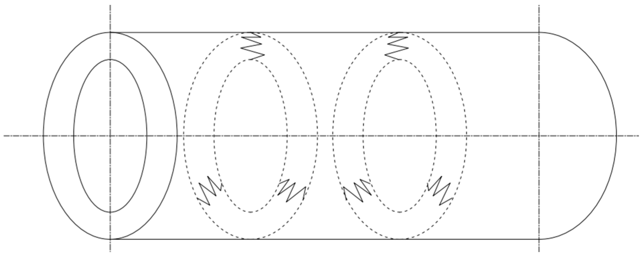
2.2. Support System

A series of reinforced supports are installed between the double-layer cylindrical shells, and each support is generally simplified as a two-force rod in mechanics. If $A_j(z_{\mathrm{A}j},{\phi }_{\mathrm{A}j},R_{\mathrm{A}})$ and $B_j(z_{\mathrm{B}j},{\phi }_{\mathrm{B}j},R_{\mathrm{B}})(j=\mathrm{1,2},\dots ,N)$ are the installation points of the support and shells A and B, respectively, then the transmitted force of each support is only along the direction of $\overrightarrow{B_j{A}_j}$ or $\overrightarrow{{A_{j}B}_j}$. As a vibration reduction design scheme, these supports are composed of passive elastic supports and active actuators in parallel, and the forces exerted by each support on the A and B shells are denoted as $F_{\mathrm{A}j},F_{\mathrm{B}j}(j=\mathrm{1,2},\dots ,N)$, then

$$F_{\mathrm{A}j}=F_{\mathrm{I}\mathrm{A}j}+F_{\mathrm{d}j},F_{\mathrm{B}j}=F_{\mathrm{I}\mathrm{B}j}+F_{\mathrm{d}j}$$

(9)

In the formula, $F_{\mathrm{I}\mathrm{A}j}$ and $F_{\mathrm{I}\mathrm{B}j}$ are the forces exerted by passive support on shells A and B, respectively, while $F_{\mathrm{d}}$ is the driving force output by the actuator.

The passive support is linearly elastic, and its transmission characteristic are generally expressed using the four terminal parameter method, that is

$$\left[\begin{array}{c}{\mathit{F}}_{\mathrm{I}\mathrm{A}}\\ {\mathrm{j}\omega \mathit{X}}_{\mathrm{A}}\end{array}\right]=\left[\begin{array}{cc}{\mathit{\beta }}_{11}& {\mathit{\beta }}_{12}\\ {\mathit{\beta }}_{21}& {\mathit{\beta }}_{22}\end{array}\right]\left[\begin{array}{c}{\mathit{F}}_{\mathrm{I}\mathrm{B}}\\ \mathrm{j}\omega {\mathit{X}}_{\mathrm{B}}\end{array}\right]$$

(10)

In the formula, ${\mathit{\beta }}_{rs}=\mathrm{d}\mathrm{i}\mathrm{a}\mathrm{g}[{\beta }_{rs}^{(1)},{\beta }_{rs}^{(2)},\dots ,{\beta }_{rs}^{(N)}](r,s=\mathrm{1,2}),{\beta }_{\mathrm{r}\mathrm{s}}^{(\mathrm{j})}(j=\mathrm{1,2},\dots ,N)$ is the four terminal parameter of the $j$-th passive support; ${\mathit{F}}_{\mathrm{I}\mathrm{A}}={[F_{\mathrm{I}\mathrm{A}1},F_{\mathrm{I}\mathrm{A}2},\dots ,F_{\mathrm{I}\mathrm{A}N}]}^{\mathrm{T}}$, ${\mathit{F}}_{\mathrm{I}\mathrm{B}}={[F_{\mathrm{I}\mathrm{B}1},F_{\mathrm{I}\mathrm{B}2},\dots ,F_{\mathrm{I}\mathrm{B}N}]}^{\mathrm{T}}$; ${\mathit{X}}_{\mathrm{A}}{=[X_{\mathrm{A}1},X_{\mathrm{A}2},X_{\mathrm{A}3},\dots ,X_{\mathrm{A}N}]}^{\mathrm{T}}$, ${\mathit{X}}_{\mathrm{B}}{=[X_{\mathrm{B}1},X_{\mathrm{B}2},X_{\mathrm{B}3},\dots ,X_{\mathrm{B}N}]}^{\mathrm{T}}$; $X_{\mathrm{A}j}$, ${ X}_{\mathrm{B}j}$ represent the vibration displacement along the support direction ($\overrightarrow{{A_{j}B}_j}$) at the connection points and between each support and the shells A and B, respectively.

For each active actuator installed between the inner and outer shells, they are equipped with corresponding sensors and controllers to form an active control unit. In order to maintain generality, a classical electromagnetic actuation model is adopted for each actuator, ignoring its mass, as shown in the following equation:

$$F_{\mathrm{d}j}={\displaystyle \frac{k_{\mathrm{a}j}}{R_j+\mathrm{j}\omega L_J}}{U}_j={\displaystyle \frac{k_{\mathrm{a}j}}{R_j\left(1+\mathrm{j}\omega {\tau }_{\mathrm{a}j}\right)}}{U}_j,(j=\mathrm{1,2},\dots ,N)$$

(11)

In the formula, $U_j$ is the control voltage, $R_j$, $L_j,$ and $k_{\mathrm{a}j}$ are the driving circuit resistance, inductance, and control force output coefficient of the $j$-th active actuator, respectively, and ${\tau }_{\mathrm{a}j}$ is the electrical time constant of the active actuator.

Assuming the system adopts a linear feedback control mode, the control voltage is a linear combination of the absolute displacement, velocity, and acceleration at the connection point between the actuator and the outer shell B, as well as the relative displacement, velocity, and acceleration relative to the connection point of the inner shell A [18], that is

$$U_j{\mathrm{e}}^{-\mathrm{j}\omega {\tau }_j^{\prime }}=g_1{X}_{\mathrm{B}j}+\mathrm{j}\omega g_2{X}_{\mathrm{B}j}-{\omega }^2{g}_3{X}_{\mathrm{B}j}+g_4(X_{\mathrm{A}j}-X_{\mathrm{B}j})+\mathrm{j}\omega g_5(X_{\mathrm{A}j}-X_{\mathrm{B}j})-{\omega }^2{g}_6(X_{\mathrm{A}j}-X_{\mathrm{B}j})$$

(12)

In the formula, $g_1$, $g_2$, $g_3$, $g_4$, ${ g}_5$, ${ g}_6$ are the controller gains corresponding to each feedback signal, and ${\tau }_j^{\prime }$ is the delay compensation generated by the controller.

Substitute Equation (12) into Equation (11) and organize it into

$$\begin{array}{c}{F}_{\mathrm{d}\mathrm{j}}={\displaystyle \frac{k_{\mathrm{a}j}{\mathrm{e}}^{\mathrm{j}\omega {\tau }_j^{\prime }}}{R_j(1+\mathrm{j}\omega {\tau }_{\mathrm{a}j})}}(g_4+\mathrm{j}\omega g_5-{\omega }^2{g}_6)X_{\mathrm{A}j}+{\displaystyle \frac{k_{\mathrm{a}j}{\mathrm{e}}^{\mathrm{j}\omega {\tau }_j^{\prime }}}{R_j(1+\mathrm{j}\omega {\tau }_{\mathrm{a}j})}}[(g_1-g_4)+\mathrm{j}\omega (g_2-g_5)-{\omega }^2(g_3-g_6)]X_{\mathrm{B}j}\\ =Z_{\mathrm{A}}^{(j)}{X}_{\mathrm{A}j}+Z_{\mathrm{B}}^{(j)}{X}_{\mathrm{B}j}\end{array}$$

(13)

Extend the above equation into a form of multi actuator coupling

$${\mathit{F}}_{\mathrm{d}}={\mathit{Z}}_{\mathrm{A}}{\mathit{X}}_{\mathrm{A}}+{\mathit{Z}}_{\mathrm{B}}{\mathit{X}}_{\mathrm{B}}$$

(14)

In the formula, ${\mathit{F}}_{\mathrm{d}}={[F_{\mathrm{d}1},F_{\mathrm{d}2},\dots ,F_{\mathrm{d}N}]}^{\mathrm{T}}$, ${\mathit{Z}}_{\mathrm{A}}={\mathit{G}}_4+\mathrm{j}\omega {\mathit{G}}_5-{{\omega }^2\mathit{G}}_6$, ${\mathit{Z}}_{\mathrm{B}}=({\mathit{G}}_1-{\mathit{G}}_4)+\mathrm{j}\omega ({\mathit{G}}_2-{\mathit{G}}_5)-{\omega }^2({\mathit{G}}_3-{\mathit{G}}_6)$, ${\mathit{G}}_1$, ${\mathit{G}}_2$, ${\mathit{G}}_3$, ${\mathit{G}}_4$, ${\mathit{G}}_5$, ${\mathit{G}}_6$ are the displacement, velocity, acceleration at the connection between each actuator and the outer shell B, as well as the feedback control parameter matrix of their displacement, velocity, and acceleration relative to the connection of the inner shell A, then

$${\mathit{G}}_k=\left[\begin{array}{c}{\displaystyle \frac{{\mathrm{k}}_{\mathrm{a}1}\mathrm{e}\mathrm{x}\mathrm{p}(\mathrm{j}{\tau }_1^{\prime }\omega )}{R_1(1+\mathrm{j}{\tau }_{\mathrm{a}1}\omega )}}{g}_{11}^{(k)}\\ {\displaystyle \frac{{\mathrm{k}}_{\mathrm{a}2}\mathrm{e}\mathrm{x}\mathrm{p}(\mathrm{j}{\tau }_2^{\prime }\omega )}{R_2(1+\mathrm{j}{\tau }_{\mathrm{a}2}\omega )}}{g}_{21}^{(k)}\\ ···\\ {\displaystyle \frac{{\mathrm{k}}_{\mathrm{a}N}\mathrm{e}\mathrm{x}\mathrm{p}(\mathrm{j}{\tau }_N^{\prime }\omega )}{R_N(1+\mathrm{j}{\tau }_{\mathrm{a}N}\omega )}}{g}_{N1}^{(k)}\end{array}\begin{array}{c}{\displaystyle \frac{{\mathrm{k}}_{\mathrm{a}1}\mathrm{e}\mathrm{x}\mathrm{p}(\mathrm{j}{\tau }_1^{\prime }\omega )}{R_1(1+\mathrm{j}{\tau }_{\mathrm{a}1}\omega )}}{g}_{12}^{(k)}\\ {\displaystyle \frac{{\mathrm{k}}_{\mathrm{a}2}\mathrm{e}\mathrm{x}\mathrm{p}(\mathrm{j}{\tau }_2^{\prime }\omega )}{R_2(1+\mathrm{j}{\tau }_{\mathrm{a}2}\omega )}}{g}_{22}^{(k)}\\ ···\\ {\displaystyle \frac{{\mathrm{k}}_{\mathrm{a}N}\mathrm{e}\mathrm{x}\mathrm{p}(\mathrm{j}{\tau }_N^{\prime }\omega )}{R_N(1+\mathrm{j}{\tau }_{\mathrm{a}N}\omega )}}{g}_{N2}^{(k)}\end{array}\begin{array}{c}···\\ ···\\ ···\\ ···\end{array}\begin{array}{c}{\displaystyle \frac{{\mathrm{k}}_{\mathrm{a}1}\mathrm{e}\mathrm{x}\mathrm{p}(\mathrm{j}{\tau }_1^{\prime }\omega )}{R_1(1+\mathrm{j}{\tau }_{\mathrm{a}1}\omega )}}{g}_{1N}^{(k)}\\ {\displaystyle \frac{{\mathrm{k}}_{\mathrm{a}2}\mathrm{e}\mathrm{x}\mathrm{p}(\mathrm{j}{\tau }_2^{\prime }\omega )}{R_2(1+\mathrm{j}{\tau }_{\mathrm{a}2}\omega )}}{g}_{2N}^{(k)}\\ ···\\ {\displaystyle \frac{{\mathrm{k}}_{\mathrm{a}N}\mathrm{e}\mathrm{x}\mathrm{p}(\mathrm{j}{\tau }_N^{\prime }\omega )}{R_N(1+\mathrm{j}{\tau }_{\mathrm{a}N}\omega )}}{g}_{NN}^{(k)}\end{array}\right], (k=1, 2, 3, 4, 5, 6)$$

(15)

In the formula, $g_{ij}^{(k)}$ refers to the feedback signal collected by the sensor at the $j$-th actuator installation point, which affects the controller gain of the $i$-th actuator $(i,j=\mathrm{1,2},\dots ,N)$.

Note that ${\mathit{F}}_{\mathrm{A}}={\mathit{F}}_{\mathrm{I}\mathrm{A}}+{\mathit{F}}_{\mathrm{d}}$, ${\mathit{F}}_{\mathrm{B}}={\mathit{F}}_{\mathrm{I}\mathrm{B}}+{\mathit{F}}_{\mathrm{d}}$, combining Equations (10) and (14), yields the four terminal parameter expression for the active actuator in parallel with the passive elastic support, then

$$\left[\begin{array}{c}{\mathit{F}}_{\mathrm{I}\mathrm{A}}\\ {\mathrm{j}\omega \mathit{X}}_{\mathrm{A}}\end{array}\right]=\left[\begin{array}{cc}{\mathit{S}}_{11}& {\mathit{S}}_{12}\\ {\mathit{S}}_{21}& {\mathit{S}}_{22}\end{array}\right]\left[\begin{array}{c}{\mathit{F}}_{\mathrm{I}\mathrm{B}}\\ \mathrm{j}\omega {\mathit{X}}_{\mathrm{B}}\end{array}\right]$$

(16)

and

$$\left\{\begin{array}{c}{\mathit{S}}_{11}=({\displaystyle \frac{{\mathit{Z}}_{\mathrm{A}}}{\mathrm{j}\omega }}+{\mathit{\beta }}_{11}{\mathit{\beta }}_{21}^{-1}){(\mathit{E}+{\mathit{\beta }}_{21}{\displaystyle \frac{{\mathit{Z}}_{\mathrm{A}}}{\mathrm{j}\omega }})}^{-1}{\mathit{\beta }}_{21}\\ {\mathit{S}}_{12}={\mathit{\beta }}_{12}-{\mathit{\beta }}_{11}{\mathit{\beta }}_{21}^{-1}{\mathit{\beta }}_{22}+{\displaystyle \frac{{\mathit{Z}}_{\mathrm{B}}}{\mathrm{j}\omega }}+({\displaystyle \frac{{\mathit{Z}}_{\mathrm{A}}}{\mathrm{j}\omega }}+{\mathit{\beta }}_{11}{\mathit{\beta }}_{21}^{-1}){(\mathit{E}+{\mathit{\beta }}_{21}{\displaystyle \frac{{\mathit{Z}}_{\mathrm{A}}}{\mathrm{j}\omega }})}^{-1}({\mathit{\beta }}_{22}-{\mathit{\beta }}_{21}{\displaystyle \frac{{\mathit{Z}}_{\mathrm{B}}}{\mathrm{j}\omega }})\\ {\mathit{S}}_{21}={(\mathit{E}+{\mathit{\beta }}_{21}{\displaystyle \frac{{\mathit{Z}}_{\mathrm{A}}}{\mathrm{j}\omega }})}^{-1}{\mathit{\beta }}_{21}\\ {\mathit{S}}_{22}={(\mathit{E}+{\mathit{\beta }}_{21}{\displaystyle \frac{{\mathit{Z}}_{\mathrm{A}}}{\mathrm{j}\omega }})}^{-1}({\mathit{\beta }}_{22}-{\mathit{\beta }}_{21}{\displaystyle \frac{{\mathit{Z}}_{\mathrm{B}}}{\mathrm{j}\omega }})\end{array}\right.$$

(17)

In the formula, $\mathit{E}$ is the identity matrix.

Passive elastic support is usually regarded as a linear elastic element without quality, and its four terminal parameter ${\beta }_{11}^{(j)}={\beta }_{22}^{(j)}=1$, ${ \beta }_{12}^{(j)}=0$, ${ \beta }_{21}^{(j)}=\mathrm{j}\omega /[k^{(j)}(1+\mathrm{j}{\eta }^{(j)})]$, where $k^{(j)}(1+\mathrm{j}{\eta }^{(j)})$ is the complex stiffness of the $j$-th passive elastic support. ${\eta }^{(j)}$ is the structural damping loss factor.

In this way, Equation (17) can be simplified as

$${\mathit{S}}_{11}=\mathit{E},{\mathit{S}}_{12}=\mathit{O},{\mathit{S}}_{21}={({\mathit{\beta }}_{21}^{-1}+{\displaystyle \frac{{\mathit{Z}}_{\mathrm{A}}}{\mathrm{j}\omega }})}^{-1},{\mathit{S}}_{22}={\mathit{S}}_{21}({\mathit{\beta }}_{21}^{-1}-{\displaystyle \frac{{\mathit{Z}}_{\mathrm{B}}}{\mathrm{j}\omega }})$$

(18)

In the formula, $\mathit{O}$ is a zero matrix.

2.3. Integrated Solution of Coupled System

The cylindrical thin shell A is set as a vibration source structure here, which is simultaneously subjected to the excitation force $f_{\mathrm{e}}(z,\phi ,r,t)$ of the vibration source and the excitation force ${\mathit{F}}_{\mathrm{I}\mathrm{A}}$ of the supporting structure. According to Saint David’s principle, the excitation $f_{\mathrm{e}}(z,\phi ,r,t)$ of the vibration source is regarded as several concentrated excitation forces acting on the middle surface of shell A, listed in ${\mathit{F}}_{\mathrm{e}}={[F_{\mathrm{e}1},F_{\mathrm{e}2},\dots ,F_{\mathrm{e}{N}^{\prime }}]}^{\mathrm{T}}$($N^{\prime }$ is the number of concentrated excitation forces). In addition, the displacement response of shell A along the direction of the excitation force at the above excitation point is listed in ${\mathit{X}}_{\mathrm{e}}={[X_{\mathrm{e}1},X_{\mathrm{e}2},\dots ,X_{\mathrm{e}{N}^{\prime }}]}^{\mathrm{T}}$. The relationship between ${\mathit{X}}_{\mathrm{e}}$, ${\mathit{X}}_{\mathrm{A}}$, ${\mathit{F}}_{\mathrm{e}}$ and ${\mathit{F}}_{\mathrm{I}\mathrm{A}}$ can be expressed by the directional displacement admittance function, as follows

$$\left[\begin{array}{c}{\mathit{X}}_{\mathrm{e}}\\ {\mathit{X}}_{\mathrm{A}}\end{array}\right]=\left[\begin{array}{cc}{\overline{\mathit{Y}}}_{\mathrm{A}\mathrm{e}}& {\overline{\mathit{Y}}}_{\mathrm{A}\mathrm{e}\mathrm{I}}\\ {\overline{\mathit{Y}}}_{\mathrm{A}\mathrm{I}\mathrm{e}}& {\overline{\mathit{Y}}}_{\mathrm{A}\mathrm{I}}\end{array}\right]\left[\begin{array}{c}{\mathit{F}}_{\mathrm{e}}\\ {\mathit{F}}_{\mathrm{I}\mathrm{A}}\end{array}\right]={\overline{\mathit{Y}}}_{\mathrm{A}}\left[\begin{array}{c}{\mathit{F}}_{\mathrm{e}}\\ {\mathit{F}}_{\mathrm{I}\mathrm{A}}\end{array}\right]$$

(19)

From the perspective of vibration transmission process, the cylindrical thin shell B is located at the end of the entire transmission path, serving as the receptor and only subjected to the excitation force ${\mathit{F}}_{\mathrm{I}\mathrm{B}}$ of the supporting structure. The transmission relationship between the excitation force ${\mathit{F}}_{\mathrm{I}\mathrm{B}}$ of the supporting structure and the vibration displacement response ${\mathit{X}}_{\mathrm{B}}$ of the supporting installation position (along the supporting direction) on the B shell is also expressed by the directional displacement admittance matrix similar to ${\overline{\mathit{Y}}}_{\mathrm{A}\mathrm{I}}$

$${\mathit{X}}_{\mathrm{B}}={\overline{\mathit{Y}}}_{\mathrm{B}}·{\mathit{F}}_{\mathrm{I}\mathrm{B}}$$

(20)

By using Equations (16), (19) and (20), the vibration response and ${\mathit{X}}_{\mathrm{e}}$, ${\mathit{X}}_{\mathrm{A}}$, ${\mathit{X}}_{\mathrm{B}}$ dynamic transmission force ${\mathit{F}}_{\mathrm{I}\mathrm{A}}$, ${\mathit{F}}_{\mathrm{I}\mathrm{B}}$ of the coupled system can be derived, and the dependence relationship between the two and the excitation ${\mathit{F}}_{\mathrm{e}}$ of the vibration source can be established

$$\left\{\begin{array}{c}{\mathbf{X}}_{\mathrm{e}}=[{\overline{\mathit{Y}}}_{\mathrm{A}\mathrm{e}}+{\overline{\mathit{Y}}}_{\mathrm{A}\mathrm{e}\mathrm{I}}{({\displaystyle \frac{{\mathit{S}}_{21}-{\overline{\mathit{Y}}}_{\mathrm{A}\mathrm{I}}}{\mathrm{j}\omega }}+{\mathit{S}}_{22}{\overline{\mathit{Y}}}_{\mathrm{B}})}^{-1}{\overline{\mathit{Y}}}_{\mathrm{A}\mathrm{I}\mathrm{e}}]{\mathit{F}}_{\mathrm{e}}\\ {\mathbf{X}}_{\mathrm{A}}=({\mathit{S}}_{21}+\mathrm{j}\omega {\mathit{S}}_{22}{\overline{\mathit{Y}}}_{\mathrm{B}})·{({\displaystyle \frac{{\mathit{S}}_{21}-{\overline{\mathit{Y}}}_{\mathrm{A}\mathrm{I}}}{\mathrm{j}\omega }}+{\mathit{S}}_{22}{\overline{\mathit{Y}}}_{\mathrm{B}})}^{-1}{\overline{\mathit{Y}}}_{\mathrm{A}\mathrm{I}\mathrm{e}}{\mathit{F}}_{\mathrm{e}}\\ {\mathbf{X}}_{\mathrm{B}}={\overline{\mathit{Y}}}_{\mathrm{B}}{({\displaystyle \frac{{\mathit{S}}_{21}-{\overline{\mathit{Y}}}_{\mathrm{A}\mathrm{I}}}{\mathrm{j}\omega }}+{\mathit{S}}_{22}{\overline{\mathit{Y}}}_{\mathrm{B}})}^{-1}{\overline{\mathit{Y}}}_{\mathrm{A}\mathrm{I}\mathrm{e}}{\mathit{F}}_{\mathrm{e}}\\ {\mathbf{F}}_{\mathrm{I}\mathrm{A}}={\mathbf{F}}_{\mathrm{I}\mathrm{B}}={({\displaystyle \frac{{\mathit{S}}_{21}-{\overline{\mathit{Y}}}_{\mathrm{A}\mathrm{I}}}{\mathrm{j}\omega }}+{\mathit{S}}_{22}{\overline{\mathit{Y}}}_{\mathrm{B}})}^{-1}{\overline{\mathit{Y}}}_{\mathrm{A}\mathrm{I}\mathrm{e}}{\mathit{F}}_{\mathrm{e}}\end{array}\right.$$

(21)

In Equations (19)–(21), ${\overline{\mathit{Y}}}_{\mathrm{A}\mathrm{e}}$, ${\overline{\mathit{Y}}}_{\mathrm{A}\mathrm{e}\mathrm{I}}$, ${\overline{\mathit{Y}}}_{\mathrm{A}\mathrm{I}\mathrm{e}}$, ${\overline{\mathit{Y}}}_{\mathrm{A}\mathrm{I}}$, ${\overline{\mathit{Y}}}_{\mathrm{B}}$ are the displacement admittance matrices of shell A and shell B composed of directional displacement admittance functions, which are described as follows:

(1)

${\overline{\mathit{Y}}}_{\mathrm{A}\mathrm{e}}=[{\overline{Y}}_{\mathrm{A}\mathrm{e}ij}]$ is an $N^{\prime }\times N^{\prime }$ order square matrix, which describes the transitive relation between the vibration displacement response ${\mathit{X}}_{\mathrm{e}}$ at the excitation point (along the direction of the vibration source excitation) of the vibration source excitation ${\mathit{F}}_{\mathrm{e}}$ on the shell A. The point of action of the excitation force $F_{\mathrm{e}j}(j=\mathrm{1,2},\dots ,N^{\prime })$ from each vibration source is $A_{\mathrm{e}j}(z_{\mathrm{e}j},{\phi }_{\mathrm{e}j},R_{\mathrm{A}})$, and the direction of action is $\overrightarrow{d_{\mathrm{e}j}}={\mathrm{c}\mathrm{o}\mathrm{s}{\psi }_{\mathrm{e}1}}^{(j)}\overrightarrow{{\mathrm{e}}_1}+{\mathrm{c}\mathrm{o}\mathrm{s}{\psi }_{\mathrm{e}2}}^{(j)}\overrightarrow{{\mathrm{e}}_2}({\phi }_{\mathrm{e}})+{\mathrm{c}\mathrm{o}\mathrm{s}{\psi }_{\mathrm{e}3}}^{(j)}\overrightarrow{{\mathrm{e}}_3}({\phi }_{\mathrm{e}})$; ${{\psi }_{\mathrm{e}1}}^{(j)}$, ${{\psi }_{\mathrm{e}2}}^{(j)},$ and ${{\psi }_{\mathrm{e}3}}^{(j)}$ are the angles between $\overrightarrow{d_{\mathrm{e}j}}$ and the base vectors $\overrightarrow{{\mathrm{e}}_1}$, $\overrightarrow{{\mathrm{e}}_2}({\phi }_{\mathrm{e}})$, and $\overrightarrow{{\mathrm{e}}_3}({\phi }_{\mathrm{e}})$. Then, Equation (8) can be used to obtain

$${\overline{Y}}_{\mathrm{A}\mathrm{e}ij}=\left[\begin{array}{ccc}{\mathrm{c}\mathrm{o}\mathrm{s}{\psi }_1}^{(i)}& {\mathrm{c}\mathrm{o}\mathrm{s}{\psi }_2}^{(i)}& {\mathrm{c}\mathrm{o}\mathrm{s}{\psi }_3}^{(i)}\end{array}\right]\left[\begin{array}{c}{Y}_{\mathrm{A}11}(A_{\mathrm{e}i},A_{\mathrm{e}j})\\ Y_{\mathrm{A}21}(A_{\mathrm{e}i},A_{\mathrm{e}j})\\ Y_{\mathrm{A}31}(A_{\mathrm{e}i},A_{\mathrm{e}j})\end{array}\begin{array}{c}{Y}_{\mathrm{A}12}(A_{\mathrm{e}i},A_{\mathrm{e}j})\\ Y_{\mathrm{A}22}(A_{\mathrm{e}i},A_{\mathrm{e}j})\\ Y_{\mathrm{A}32}(A_{\mathrm{e}i},A_{\mathrm{e}j})\end{array}\begin{array}{c}{Y}_{\mathrm{A}13}(A_{\mathrm{e}i},A_{\mathrm{e}j})\\ Y_{\mathrm{A}23}(A_{\mathrm{e}i},A_{\mathrm{e}j})\\ Y_{\mathrm{A}33}(A_{\mathrm{e}i},A_{\mathrm{e}j})\end{array}\right]\left[\begin{array}{c}{\mathrm{c}\mathrm{o}\mathrm{s}{\psi }_{\mathrm{e}1}}^{(j)}\\ {\mathrm{c}\mathrm{o}\mathrm{s}{\psi }_{\mathrm{e}2}}^{(j)}\\ {\mathrm{c}\mathrm{o}\mathrm{s}{\psi }_{\mathrm{e}3}}^{(j)}\end{array}\right]$$

(22)

(2)

${\overline{\mathit{Y}}}_{\mathrm{A}\mathrm{e}\mathrm{I}}={\overline{[Y}}_{\mathrm{A}\mathrm{e}\mathrm{I}ij}]$ is an $N^{\prime }\times N$ order matrix, which describes the transitive relation between the vibration displacement response ${\mathit{X}}_{\mathrm{e}}$ at the point of excitation (along the direction of excitation) of the vibration source on the support excitation ${\mathit{F}}_{\mathrm{I}\mathrm{A}}$ of shell A. Given that the installation position of each support on shell A and shell B are $A_j(z_{\mathrm{A}j},{\phi }_{\mathrm{A}j},R_{\mathrm{A}})$ and $B_j(z_{\mathrm{B}j},{\phi }_{\mathrm{B}j},R_{\mathrm{B}})(j=\mathrm{1,2},\dots ,N)$, the excitation force $F_{\mathrm{I}j}$ acting on shell A is along the $\overrightarrow{B_j{A}_j}$ direction

$$\overrightarrow{B_j{A}_j}=(z_{\mathrm{A}j}-z_{\mathrm{B}j})\overrightarrow{{\mathrm{e}}_1}+R_{\mathrm{A}}\overrightarrow{{\mathrm{e}}_3}({\phi }_{\mathrm{A}j})-R_{\mathrm{B}}\overrightarrow{{\mathrm{e}}_3}({\phi }_{\mathrm{B}j})$$

(23)

Note that ${n_{\mathrm{A}1}}^{(j)}$, ${n_{\mathrm{A}2}}^{(j)}$, and ${n_{\mathrm{A}3}}^{(j)}$ are the cosine of the angle between $\overrightarrow{B_j{A}_j}$ and $\overrightarrow{{\mathrm{e}}_1}$, $\overrightarrow{{\mathrm{e}}_2}({\phi }_{\mathrm{A}j})$, and $\overrightarrow{{\mathrm{e}}_3}({\phi }_{\mathrm{A}j})$, respectively $(j=\mathrm{1,2},\dots ,N)$

$$\left\{\begin{array}{c}{n_{\mathrm{A}1}}^{(j)}={\displaystyle \frac{z_{\mathrm{A}j}-z_{\mathrm{B}j}}{\sqrt{{R_{\mathrm{A}}}^2+{R_{\mathrm{B}}}^2+{(z_{\mathrm{A}j}-z_{\mathrm{B}j})}^2-2R_{\mathrm{A}}{R}_{\mathrm{B}}\mathrm{c}\mathrm{o}\mathrm{s}({\phi }_{\mathrm{A}j}-{\phi }_{\mathrm{B}j})}}}\\ {n_{\mathrm{A}2}}^{(j)}={\displaystyle \frac{R_{\mathrm{B}}\mathrm{s}\mathrm{i}\mathrm{n}({\phi }_{\mathrm{A}\mathrm{j}}-{\phi }_{\mathrm{B}\mathrm{j}})}{\sqrt{{R_{\mathrm{A}}}^2+{R_{\mathrm{B}}}^2+{(z_{\mathrm{A}j}-z_{\mathrm{B}j})}^2-2R_{\mathrm{A}}{R}_{\mathrm{B}}\mathrm{c}\mathrm{o}\mathrm{s}({\phi }_{\mathrm{A}j}-{\phi }_{\mathrm{B}j})}}}\\ {n_{\mathrm{A}3}}^{(j)}={\displaystyle \frac{R_{\mathrm{A}}-R_{\mathrm{B}}\mathrm{c}\mathrm{o}\mathrm{s}({\phi }_{\mathrm{A}\mathrm{j}}-{\phi }_{\mathrm{B}\mathrm{j}})}{\sqrt{{R_{\mathrm{A}}}^2+{R_{\mathrm{B}}}^2+{(z_{\mathrm{A}j}-z_{\mathrm{B}j})}^2-2R_{\mathrm{A}}{R}_{\mathrm{B}}\mathrm{c}\mathrm{o}\mathrm{s}({\phi }_{\mathrm{A}j}-{\phi }_{\mathrm{B}j})}}}\end{array}\right.$$

(24)

So according to Equation (8), we can obtain

$$\begin{array}{c}{\overline{Y}}_{\mathrm{A}\mathrm{e}\mathrm{I}ij}={\overline{Y}}_{\mathrm{A}}(A_{\mathrm{e}i},\overrightarrow{d_{\mathrm{e}i}};A_j,{n_{\mathrm{A}1}}^{(j)}\overrightarrow{{\mathrm{e}}_1}+{n_{\mathrm{A}2}}^{(j)}\overrightarrow{{\mathrm{e}}_2}({\phi }_{\mathrm{A}j})+{n_{\mathrm{A}3}}^{(j)}\overrightarrow{{\mathrm{e}}_3}({\phi }_{\mathrm{A}j}))\\ =\left[\begin{array}{ccc}{\mathrm{c}\mathrm{o}\mathrm{s}{\psi }_{\mathrm{e}1}}^{(j)}& {\mathrm{c}\mathrm{o}\mathrm{s}{\psi }_{\mathrm{e}2}}^{(j)}& {\mathrm{c}\mathrm{o}\mathrm{s}{\psi }_{\mathrm{e}3}}^{(j)}\end{array}\right]\left[\begin{array}{c}{Y}_{\mathrm{A}11}(A_{\mathrm{e}i},A_j)\\ Y_{\mathrm{A}21}(A_{\mathrm{e}i},A_j)\\ Y_{\mathrm{A}31}(A_{\mathrm{e}i},A_j)\end{array}\begin{array}{c}{Y}_{\mathrm{A}12}(A_{\mathrm{e}i},A_j)\\ Y_{\mathrm{A}22}(A_{\mathrm{e}i},A_j)\\ Y_{\mathrm{A}32}(A_{\mathrm{e}i},A_j)\end{array}\begin{array}{c}{Y}_{\mathrm{A}13}(A_{\mathrm{e}i},A_j)\\ Y_{\mathrm{A}23}(A_{\mathrm{e}i},A_j)\\ Y_{\mathrm{A}33}(A_{\mathrm{e}i},A_j)\end{array}\right]\left[\begin{array}{c}{n_{\mathrm{A}1}}^{(j)}\\ {n_{\mathrm{A}2}}^{(j)}\\ {n_{\mathrm{A}3}}^{(j)}\end{array}\right]\end{array}$$

(25)

(3)

${\overline{\mathit{Y}}}_{\mathrm{A}\mathrm{I}\mathrm{e}}=[{\overline{Y}}_{\mathrm{A}\mathrm{I}\mathrm{e}ij}]$ is an $N\times N^{\prime }$ order matrix, which describes the transitive relation between the vibration displacement response ${\mathit{X}}_{\mathrm{A}}$ at the support installation position (along the support direction) and the excitation ${\mathit{F}}_{\mathrm{I}\mathrm{A}}$ on shell A. Note that the displacement response ${\mathrm{X}}_{\mathrm{A}\mathrm{i}}$ at the installation position of each support on the A shell should be in the positive direction of the $\overrightarrow{{A_{i}B}_i}(i=\mathrm{1,2},\dots N)$ direction, so according to Equation (8), we can obtain

$$\begin{array}{c}{\overline{Y}}_{\mathrm{A}\mathrm{I}\mathrm{e}ij}={\overline{Y}}_{\mathrm{A}}(A_i,-{n_{\mathrm{A}1}}^{(i)}\overrightarrow{{\mathrm{e}}_1}-{n_{\mathrm{A}2}}^{(i)}\overrightarrow{{\mathrm{e}}_2}({\phi }_{\mathrm{A}i})-{n_{\mathrm{A}3}}^{(i)}\overrightarrow{{\mathrm{e}}_3}({\phi }_{\mathrm{A}i});A_{\mathrm{e}j},\overrightarrow{d_{\mathrm{e}j}})\\ =-\left[\begin{array}{ccc}{n_{\mathrm{A}1}}^{(\mathrm{i})}& {n_{\mathrm{A}2}}^{(\mathrm{i})}& {n_{\mathrm{A}3}}^{(\mathrm{i})}\end{array}\right]\left[\begin{array}{c}{\mathrm{Y}}_{\mathrm{A}11}(A_{\mathrm{e}i},A_j)\\ {\mathrm{Y}}_{\mathrm{A}21}(A_{\mathrm{e}i},A_j)\\ {\mathrm{Y}}_{\mathrm{A}31}(A_{\mathrm{e}i},A_j)\end{array}\begin{array}{c}{\mathrm{Y}}_{\mathrm{A}12}(A_{\mathrm{e}i},A_{\mathrm{j}})\\ {\mathrm{Y}}_{\mathrm{A}22}(A_{\mathrm{e}i},A_{\mathrm{j}})\\ {\mathrm{Y}}_{\mathrm{A}32}(A_{\mathrm{e}i},A_{\mathrm{j}})\end{array}\begin{array}{c}{\mathrm{Y}}_{\mathrm{A}13}(A_{\mathrm{e}i},A_j)\\ {\mathrm{Y}}_{\mathrm{A}23}(A_{\mathrm{e}i},A_j)\\ {\mathrm{Y}}_{\mathrm{A}33}(A_{\mathrm{e}i},A_j)\end{array}\right]\left[\begin{array}{c}{\mathrm{c}\mathrm{o}\mathrm{s}{\psi }_{\mathrm{e}1}}^{(j)}\\ {\mathrm{c}\mathrm{o}\mathrm{s}{\psi }_{\mathrm{e}2}}^{(j)}\\ {\mathrm{c}\mathrm{o}\mathrm{s}{\psi }_{\mathrm{e}3}}^{(j)}\end{array}\right]\end{array}$$

(26)

Comparing Equations (25) and (26), it can be seen that they have an anti-symmetric relationship, and it can be concluded that ${\overline{Y}}_{\mathrm{A}\mathrm{I}\mathrm{e}ij}=-{\overline{Y}}_{\mathrm{A}\mathrm{e}\mathrm{I}ij}$. Namely,

$${\overline{\mathit{Y}}}_{\mathrm{A}\mathrm{I}\mathrm{e}}=-{{\overline{\mathit{Y}}}_{\mathrm{A}\mathrm{I}\mathrm{e}}}^{\mathrm{T}}$$

(27)

(4)

${\overline{\mathit{Y}}}_{\mathrm{A}\mathrm{I}}=[{\overline{Y}}_{\mathrm{A}\mathrm{I}ij}]$ is an $N\times N$ order square matrix, which describes the transitive relation between the vibration source excitation ${\mathit{F}}_{\mathrm{e}}$ on the A shell and the vibration displacement response ${\mathit{X}}_{\mathrm{A}}$ at the support installation position (along the support direction). The prescribed positive direction (along $\overrightarrow{{B_{i}A}_i}$ direction) of the support excitation $F_{\mathrm{I}j}$ acting on shell A is opposite to the prescribed positive direction (along $\overrightarrow{{A_{i}B}_i}(i=\mathrm{1,2},\dots N)$ direction) of the displacement response $X_{\mathrm{A}i}$ at its position of action, so according to Equation (8), it can be obtained as

$$\begin{array}{c}{\overline{Y}}_{\mathrm{A}\mathrm{I}ij}={\overline{Y}}_{\mathrm{A}}(A_i,-{n_{\mathrm{A}1}}^{(i)}\overrightarrow{{\mathrm{e}}_1}-{n_{\mathrm{A}2}}^{(i)}\overrightarrow{{\mathrm{e}}_2}({\phi }_{\mathrm{A}i})-{n_{\mathrm{A}3}}^{(i)}\overrightarrow{{\mathrm{e}}_3}({\phi }_{\mathrm{A}i});A_j,{n_{\mathrm{A}1}}^{(j)}\overrightarrow{{\mathrm{e}}_1}+{n_{\mathrm{A}2}}^{(j)}\overrightarrow{{\mathrm{e}}_2}({\phi }_{\mathrm{A}j})+{n_{\mathrm{A}3}}^{(j)}\overrightarrow{{\mathrm{e}}_3}({\phi }_{\mathrm{A}j}))\\ =-\left[\begin{array}{ccc}{n_{\mathrm{A}1}}^{(i)}& {n_{\mathrm{A}2}}^{(i)}& {n_{\mathrm{A}3}}^{(i)}\end{array}\right]\left[\begin{array}{c}{Y}_{\mathrm{A}11}(A_i,A_j)\\ Y_{\mathrm{A}21}(A_i,A_j)\\ Y_{\mathrm{A}31}(A_i,A_j)\end{array}\begin{array}{c}{Y}_{\mathrm{A}12}(A_i,A_j)\\ Y_{\mathrm{A}22}(A_i,A_j)\\ Y_{\mathrm{A}32}(A_i,A_j)\end{array}\begin{array}{c}{Y}_{\mathrm{A}13}(A_i,A_j)\\ Y_{\mathrm{A}23}(A_i,A_j)\\ Y_{\mathrm{A}33}(A_i,A_j)\end{array}\right]\left[\begin{array}{c}{n_{\mathrm{A}1}}^{(j)}\\ {n_{\mathrm{A}2}}^{(j)}\\ {n_{\mathrm{A}3}}^{(j)}\end{array}\right]\end{array}$$

(28)

(5)

In Equation (20), ${\overline{\mathrm{Y}}}_{\mathrm{B}}=[{\overline{Y}}_{\mathrm{B}ij}]$ is an $N\times N$ order square matrix composed of directional displacement admittance ${\overline{Y}}_{\mathrm{B}ij}$, which is the displacement response $X_{\mathrm{B}i}$ along the $\overrightarrow{{A_{i}B}_i}$ direction on the B shell to the directional displacement admittance of the support excitation $F_{\mathrm{I}j}$ along the $\overrightarrow{{A_{j}B}_j}$ direction $(i,j=\mathrm{1,2},\dots ,N)$

Let ${n_{\mathrm{B}1}}^{(j)}$, ${n_{\mathrm{B}2}}^{(j)}$, and ${n_{\mathrm{B}3}}^{(j)}$ be the cosine of the angles between $\overrightarrow{{A_{j}B}_j}$ and $\overrightarrow{{\mathrm{e}}_1}$, $\overrightarrow{{\mathrm{e}}_2}({\phi }_{\mathrm{B}j})$, and $\overrightarrow{{\mathrm{e}}_3}({\phi }_{\mathrm{B}j})$, respectively

$$\left\{\begin{array}{c}{n_{\mathrm{B}1}}^{(j)}={\displaystyle \frac{-(z_{\mathrm{A}j}-z_{\mathrm{B}j})}{\sqrt{{R_{\mathrm{A}}}^2+{R_{\mathrm{B}}}^2+{(z_{\mathrm{A}j}-z_{\mathrm{B}j})}^2-2R_{\mathrm{A}}{R}_{\mathrm{B}}\mathrm{c}\mathrm{o}\mathrm{s}({\phi }_{\mathrm{A}j}-{\phi }_{\mathrm{B}j})}}}\\ {n_{\mathrm{B}2}}^{(j)}={\displaystyle \frac{{-R}_{\mathrm{A}}\mathrm{s}\mathrm{i}\mathrm{n}({\phi }_{\mathrm{A}j}-{\phi }_{\mathrm{B}j})}{\sqrt{{R_{\mathrm{A}}}^2+{R_{\mathrm{B}}}^2+{(z_{\mathrm{A}j}-z_{\mathrm{B}j})}^2-2R_{\mathrm{A}}{R}_{\mathrm{B}}\mathrm{c}\mathrm{o}\mathrm{s}({\phi }_{\mathrm{A}j}-{\phi }_{\mathrm{B}j})}}}\\ {n_{\mathrm{B}3}}^{(j)}={\displaystyle \frac{-R_{\mathrm{B}}+R_{\mathrm{A}}\mathrm{c}\mathrm{o}\mathrm{s}({\phi }_{\mathrm{A}j}-{\phi }_{\mathrm{B}j})}{\sqrt{{R_{\mathrm{A}}}^2+{R_{\mathrm{B}}}^2+{(z_{\mathrm{A}j}-z_{\mathrm{B}j})}^2-2R_{\mathrm{A}}{R}_{\mathrm{B}}\mathrm{c}\mathrm{o}\mathrm{s}({\phi }_{\mathrm{A}j}-{\phi }_{\mathrm{B}j})}}}\end{array}\right.$$

(29)

Thus, according to Equation (8), we can obtain

$$\begin{array}{c}{\overline{Y}}_{\mathrm{B}ij}={\overline{ Y}}_{\mathrm{B}}(B_i,-{n_{\mathrm{B}1}}^{(i)}\overrightarrow{{\mathrm{e}}_1}-{n_{\mathrm{B}2}}^{(i)}\overrightarrow{{\mathrm{e}}_2}({\phi }_{\mathrm{B}i})-{n_{\mathrm{B}3}}^{(i)}\overrightarrow{{\mathrm{e}}_3}({\phi }_{\mathrm{B}i});B_j,{n_{\mathrm{B}1}}^{(j)}\overrightarrow{{\mathrm{e}}_1}+{n_{\mathrm{B}2}}^{(j)}\overrightarrow{{\mathrm{e}}_2}({\phi }_{\mathrm{B}j})+{n_{\mathrm{B}3}}^{(j)}\overrightarrow{{\mathrm{e}}_3}({\phi }_{\mathrm{B}j}))\\ =\left[\begin{array}{ccc}{n_{\mathrm{B}1}}^{(i)}& {n_{\mathrm{B}2}}^{(i)}& {n_{\mathrm{B}3}}^{(i)}\end{array}\right]\left[\begin{array}{c}{Y}_{\mathrm{A}11}(B_i,B_j)\\ Y_{\mathrm{A}21}(B_i,B_j)\\ Y_{\mathrm{A}31}(B_i,B_j)\end{array}\begin{array}{c}{Y}_{\mathrm{A}12}(B_i,B_j)\\ Y_{\mathrm{A}22}(B_i,B_j)\\ Y_{\mathrm{A}32}(B_i,B_j)\end{array}\begin{array}{c}{Y}_{\mathrm{A}13}(B_i,B_j)\\ Y_{\mathrm{A}23}(B_i,B_j)\\ Y_{\mathrm{A}33}(B_i,B_j)\end{array}\right]\left[\begin{array}{c}{n_{\mathrm{B}1}}^{(j)}\\ {n_{\mathrm{B}2}}^{(j)}\\ {n_{\mathrm{B}3}}^{(j)}\end{array}\right]\end{array}$$

(30)

2.4. Vibration Power Flow

After completing the comprehensive analysis of subsystem admittance, the following is the derived transfer power flow.

For the elastic coupling system composed of cylindrical thin shell A, supporting structure, and cylindrical thin shell B mentioned above, ${{\mathit{F}}_{\mathrm{e}}=[F_{\mathrm{e}1},F_{\mathrm{e}2},F_{\mathrm{e}3},\dots ,F_{\mathrm{e}{N}^{\prime }}]}^{\mathrm{T}}$ is the vibration source excitation (harmonic excitation) acting on the A shell, and ${{\mathit{X}}_{\mathrm{e}}=[X_{\mathrm{e}1},X_{\mathrm{e}2},X_{\mathrm{e}3},\dots ,X_{\mathrm{e}{N}^{\prime }}]}^{\mathrm{T}}$ is the vibration displacement along the excitation direction corresponding to ${\mathit{F}}_{\mathrm{e}}$ at each excitation point. Therefore, the average excitation power of ${\mathit{F}}_{\mathrm{e}}$ on the A shell is

$${\mathit{P}}_{\mathrm{e}}={\sum }_{j=1}^{N^{\prime }}{\displaystyle \frac{\omega }{2\pi }}{\int }_0^{{\displaystyle \frac{2\pi }{\omega }}}\mathrm{R}\mathrm{e}[F_{\mathrm{e}i}·\mathrm{e}\mathrm{x}\mathrm{p}(\mathrm{j}\omega t)]\mathrm{R}\mathrm{e}\left\{{\displaystyle \frac{\mathrm{d}[X_{\mathrm{e}i}·\mathrm{e}\mathrm{x}\mathrm{p}(\mathrm{j}\omega t)]}{\mathrm{d}\mathrm{t}}}\right\}\mathrm{d}\mathrm{t}={\displaystyle \frac{\omega }{2}}\mathrm{I}\mathrm{m}[{\mathit{F}}_{\mathrm{e}}^{\mathrm{T}}·{\mathit{X}}_{\mathrm{e}}^{\mathrm{*}}]$$

(31)

In the formula, ${\mathit{X}}_{\mathrm{e}}^{\mathrm{*}}$ represents the conjugate of ${\mathit{X}}_{\mathrm{e}}$.

The average excitation power of ${\mathit{F}}_{\mathrm{I}\mathrm{A}}$ on shell A is

$${\mathit{P}}_{\mathrm{I}\mathrm{A}}=-{\displaystyle \frac{\omega }{2}}\mathrm{I}\mathrm{m}[{\mathit{F}}_{\mathrm{I}\mathrm{A}}^{\mathrm{T}}·{\mathit{X}}_{\mathrm{A}}^{\mathrm{*}}]$$

(32)

The average dissipated power of shell A is

$${\mathit{P}}_{\mathrm{A}}={\mathit{P}}_{\mathrm{e}}+{\mathit{P}}_{\mathrm{I}\mathrm{A}}$$

(33)

The average excitation power of ${\mathit{F}}_{\mathrm{I}\mathrm{B}}$ on the B shell is, which is the average dissipation power of the B shell

$${{\mathit{P}}_{\mathrm{I}\mathrm{B}}=\mathit{P}}_{\mathrm{B}}={\displaystyle \frac{\omega }{2}}\mathrm{I}\mathrm{m}[{\mathit{F}}_{\mathrm{I}\mathrm{B}}^{\mathrm{T}}·{\mathit{X}}_{\mathrm{B}}^{\mathrm{*}}]$$

(34)

The average dissipated power of the supporting structure is

$${{\mathit{P}}_{\mathrm{I}}=-{\mathit{P}}_{\mathrm{I}\mathrm{A}}-\mathit{P}}_{\mathrm{I}\mathrm{B}}$$

(35)

Obviously, the balance relationship of vibration energy is that the total input energy excited by the vibration source is equal to the sum of the energy dissipated by the A shell, B shell, and supporting structure, or it can be said that the total input power excited by the vibration source is equal to the sum of the power dissipated by the A shell, B shell, and supporting structure, that is

$${\mathit{P}}_{\mathrm{e}}={\mathit{P}}_{\mathrm{A}}+{\mathit{P}}_{\mathrm{B}}+{\mathit{P}}_{\mathrm{I}}$$

(36)

Due to the constant presence of damping in various structural systems, there is also significant energy dissipation during severe system vibrations. External excitation requires a continuous injection of the corresponding amount of energy into the system to sustain the vibrations. Therefore, vibration power flow can be used to evaluate the damping effect of passive active vibration control systems and provide guidance for damping design.

3. Simulation Analysis of Active Vibration Control

3.1. Simulation Model Establishment

In order to maintain generality, this paper uses the numerical simulation analysis of active vibration control of a double-layer cylindrical thin shell containing active actuators using the example model in Figure 2 [27]. Compared to other structures such as active vibration control based on piezoelectric intelligent structures in the past, it can provide greater control force, thereby achieving better mid to low frequency vibration control effects.

In Figure 2, there is a unit concentrated harmonic excitation acting radially at point $(1,0°,R_{\mathrm{A}})$ on shell A; $N=6$ active control units were installed uniformly along the radial direction, and their installation positions on shells A and B are respectively

$$\begin{array}{c}{A}_1(0.65,0°,R_{\mathrm{A}}),A_2(0.65,120°,R_{\mathrm{A}}),A_3(0.65,-120°,R_{\mathrm{A}})\\ A_4(1.35,0°,R_{\mathrm{A}}),A_5(1.35,120°,R_{\mathrm{A}}),A_6(1.35,-120°,R_{\mathrm{A}})\end{array}$$

as well as

$$\begin{array}{c}{B}_1(0.65,0°,R_{\mathrm{B}}),B_2(0.65,120°,R_{\mathrm{B}}),B_3(0.65,-120°,R_{\mathrm{B}})\\ B_4(1.35,0°,R_{\mathrm{B}}),B_5(1.35,120°,R_{\mathrm{B}}),B_6(1.35,-120°,R_{\mathrm{B}})\end{array}$$

This coupling system uses 6 active actuators to support it, distributed in a 2 × 3 equidistant manner; that is, it surrounds the double-layer cylindrical thin shell in two circles, with three active actuators per circle and evenly distributed. For the purpose of analyzing and calculating the modal parameters of cylindrical shells A and B, it is assumed that they have simply supported boundaries, where the circumferential ($\phi$ direction) and radial ($r$ direction) deformations at their $z=0$ and $z=L$ boundaries are completely restricted, while the longitudinal direction ($z$ direction) of the boundary and the deflection of the normal outside the end face are not constrained (there is no longitudinal tensile pressure or bending moment on the end face). The natural frequencies, mode functions, and modal masses of each order obtained are shown in Appendix B.

The geometric structure parameters of cylindrical thin shells are shown in

Table 1. Geometric structural parameters of double-layer cylindrical thin shell.

Structural Parameters	Symbols	Units	Values	Remarks
Cylinder height	L	m	2
Inner shell thickness	$h_A$	m	0.015
Inner shell thickness	$h_B$	m	0.01
Inner shell thickness intermediate radius	$R_A$	m	0.35
Inner shell thickness intermediate radius	$R_B$	m	0.4

, material characteristic parameters are shown in

Table 2. Material characteristic parameter.

Material Characteristic Parameter	Symbols	Units	Values	Remarks
Poisson’s ratio	$\mu$	non	$0.3$	${\mu }_{\mathrm{A}}={\mu }_{\mathrm{B}}=\mu$
Elastic modulus	$E$	Pa	$2.1\times {10}^{11}$	${\mathrm{E}}_{\mathrm{A}}={\mathrm{E}}_{\mathrm{B}}=\mathrm{E}$
Material density	$\rho$	$\mathrm{k}\mathrm{g}/{\mathrm{m}}^3$	$7800$	${\rho }_{\mathrm{A}}={\rho }_{\mathrm{B}}=\rho$

, and active control unit characteristic parameters are shown in

Table 3. Characteristic parameters of active control unit.

Characteristic Parameters	Symbols	Units	Values	Remarks
Drive circuit resistance	$R$	$\Omega$	$2\times {10}^4$	${\mathrm{R}}_1={\mathrm{R}}_2={\mathrm{R}}_3={\mathrm{R}}_4={\mathrm{R}}_5={\mathrm{R}}_6=\mathrm{R}$
Electrical time constant	${\tau }_{\mathrm{a}}$		$5\times {10}^{-4}$	${\tau }_{\mathrm{a}1}={\tau }_{\mathrm{a}2}={\tau }_{\mathrm{a}3}={\tau }_{\mathrm{a}4}={\tau }_{\mathrm{a}5}={\tau }_{\mathrm{a}6}={\tau }_{\mathrm{a}}$
Control force output coefficient	$k_{\mathrm{a}}$		1.1	${\mathrm{k}}_{\mathrm{a}1}={\mathrm{k}}_{\mathrm{a}2}={\mathrm{k}}_{\mathrm{a}3}={\mathrm{k}}_{\mathrm{a}4}={\mathrm{k}}_{\mathrm{a}5}={\mathrm{k}}_{\mathrm{a}6}={\mathrm{k}}_{\mathrm{a}}$
Time delay	${\tau }^{\prime }$	s	$1\times {10}^{-3}$	${\tau }_1^{\prime }={\tau }_2^{\prime }={\tau }_3^{\prime }={\tau }_4^{\prime }={\tau }_5^{\prime }={\tau }_6^{\prime }={\tau }^{\prime }$
Controlled gain	$g_{\mathrm{r}\mathrm{s}}$			$(\mathrm{r},\mathrm{s}=\mathrm{1,2},\mathrm{3,4},\mathrm{5,6})$
Support stiffness	$k$	$\mathrm{N}/\mathrm{m}$		${\mathrm{k}}_1={\mathrm{k}}_2={\mathrm{k}}_3={\mathrm{k}}_4={\mathrm{k}}_5={\mathrm{k}}_6=\mathrm{k}$
Structural damping loss factor	$\eta$		0.01

and

Table 4. Controller gain values for six feedback control parameters.

Controller Gain Values	k = 1	k = 2	k = 3	k = 4	k = 5	k = 6
${\mathrm{g}}_{11}^{(\mathrm{k})}$	$\pm 1\times {10}^{10}$	$\pm 1\times {10}^9$	$\pm 1\times {10}^7$	$\pm 1\times {10}^9$	$\pm 1\times {10}^6$	$\pm 1\times {10}^2$

, as follows

3.2. Definition of Active Feedback Parameters

The sensors, controllers, actuators, and elastic supports of each active control unit use the same specifications: elastic support stiffness $k_1=k_2=k_3=k_4=k_5=k_6=k$, drive circuit resistance of active actuator $R_1=R_2=R_3=R_4={ R}_5=R_6=R$, electrical time constant ${\tau }_{\mathrm{a}1}={ \tau }_{\mathrm{a}2}={ \tau }_{\mathrm{a}3}={ \tau }_{\mathrm{a}4}={\tau }_{\mathrm{a}5}={\tau }_{\mathrm{a}6}={\tau }_{\mathrm{a}}$, control force output coefficient $k_{\mathrm{a}1}=k_{\mathrm{a}2}=k_{\mathrm{a}3}=k_{\mathrm{a}4}=k_{\mathrm{a}5}=k_{\mathrm{a}6}=k_{\mathrm{a}}$, time delay ${\tau }_1^{\prime }={\tau }_2^{\prime }={\tau }_3^{\prime }={\tau }_4^{\prime }={\tau }_5^{\prime }={\tau }_6^{\prime }={\tau }^{\prime }$. In addition, due to the complexity of considering the controlled gain of the active actuator receiving feedback signals from other installation points, this situation will be discussed later in Section 3.3.4.

Let $K={\displaystyle \raisebox{1ex}{$k_{\mathrm{a}}$}\!\left/ \!\raisebox{-1ex}{$(1+\mathrm{j}{\tau }_{\mathrm{a}}\omega )$}\right.}$, $N=6$, simplify Equation (15) as

$${\mathit{G}}_k={\displaystyle \frac{K}{R}}·\mathrm{d}\mathrm{i}\mathrm{a}\mathrm{g}[g_{11}^{(k)},g_{22}^{(k)},g_{33}^{(k)},g_{44}^{(k)},g_{55}^{(k)},g_{66}^{(k)}](k=\mathrm{1,2},\mathrm{3,4},\mathrm{5,6})$$

(37)

For the convenience of discussion, except for $g_{11}^{(k)}=g_{22}^{(k)}=g_{33}^{(k)}=g_{44}^{(k)}=g_{55}^{(k)}=g_{66}^{(k)}=g_{11}$(the sensors, controllers, and actuators in the active control unit set in the system are all of the same specifications and symmetrically arranged, so they are equal), $g_{ij}^{(k)}=0(i,j,k=\mathrm{1,2},\mathrm{3,4},\mathrm{5,6},i\ne j)$. The feedback control parameter matrix ${\mathit{G}}_k$ is only related to $g_{11}^{(k)}$, and the common part of the matrix that does not vary with frequency is defined as the feedback control parameter:

Absolute displacement feedback parameter: ${\zeta }_1={\displaystyle \frac{k_{\mathrm{a}}}{R}}{g}_{11}^{(1)}/\overline{k},\overline{k}=E·h^3/(12·(1-{\mu }^2))$.

Absolute velocity feedback parameter: ${\zeta }_2={\displaystyle \frac{k_{\mathrm{a}}}{R}}{g}_{11}^{(2)}·\eta ,\eta \in (\mathrm{0,1}]$.

Absolute acceleration feedback parameter: ${\zeta }_3={\displaystyle \frac{k_{\mathrm{a}}}{R}}{g}_{11}^{(3)}/m,m=2\pi RhL\rho$.

Relative displacement feedback parameter: ${\zeta }_4={\displaystyle \frac{k_{\mathrm{a}}}{R}}{g}_{11}^{(4)}/\overline{k}$.

Relative velocity feedback parameter: ${\zeta }_5={\displaystyle \frac{k_{\mathrm{a}}}{R}}{g}_{11}^{(5)}·\eta ,\eta \in (\mathrm{0,1}]$.

Relative acceleration feedback parameter: ${\zeta }_6={\displaystyle \frac{k_{\mathrm{a}}}{ R}}{g}_{11}^{(6)}/m$.

The feedback parameters are synthesized from the parts of the feedback control parameter matrix that do not vary with frequency, the feedback control parameter matrix with parameters is measured, reasonable values are taken, and the control effect is compared through MATLAB 2024a simulation analysis.

3.3. Analysis and Discussion of Different Feedback Control Methods

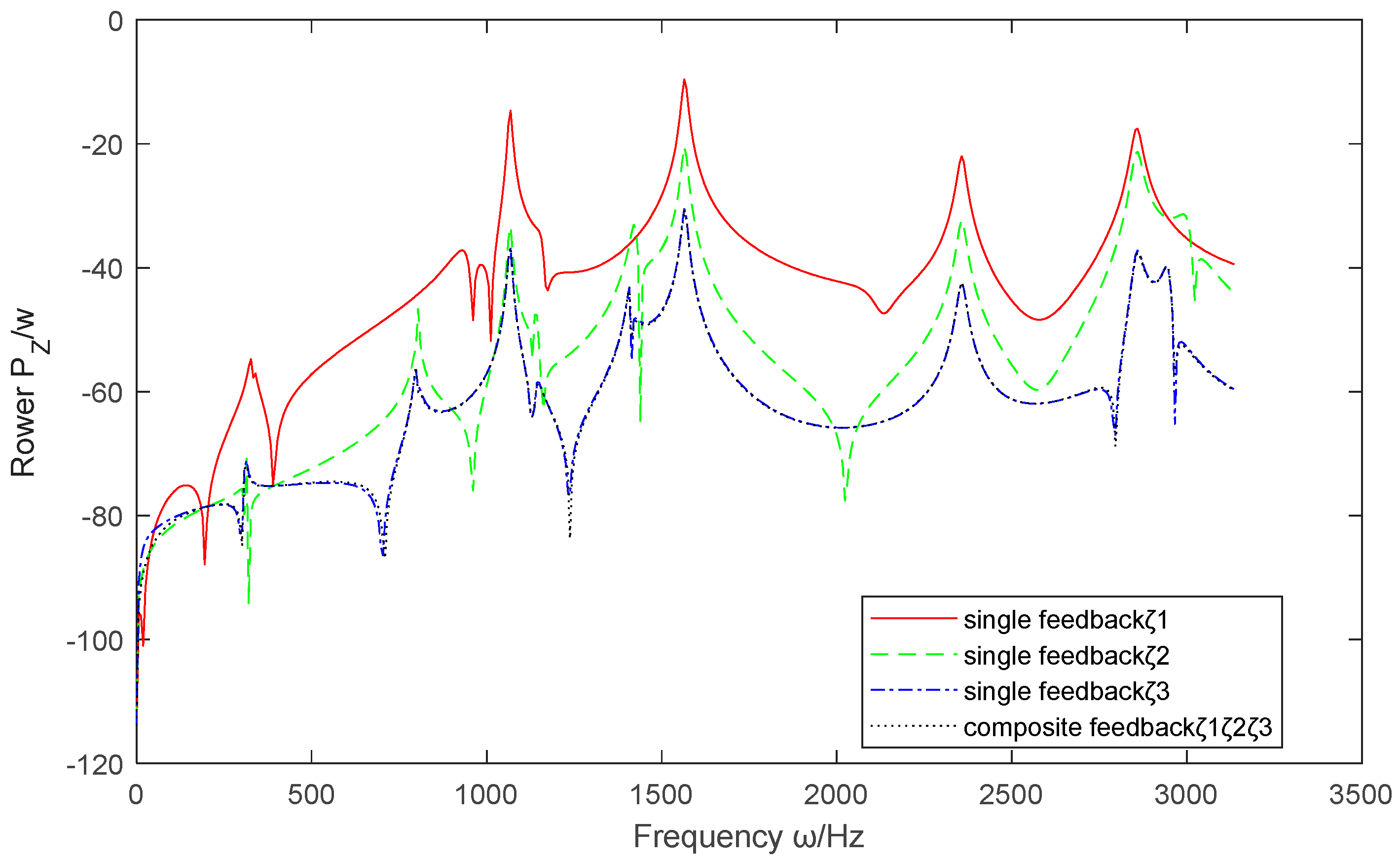
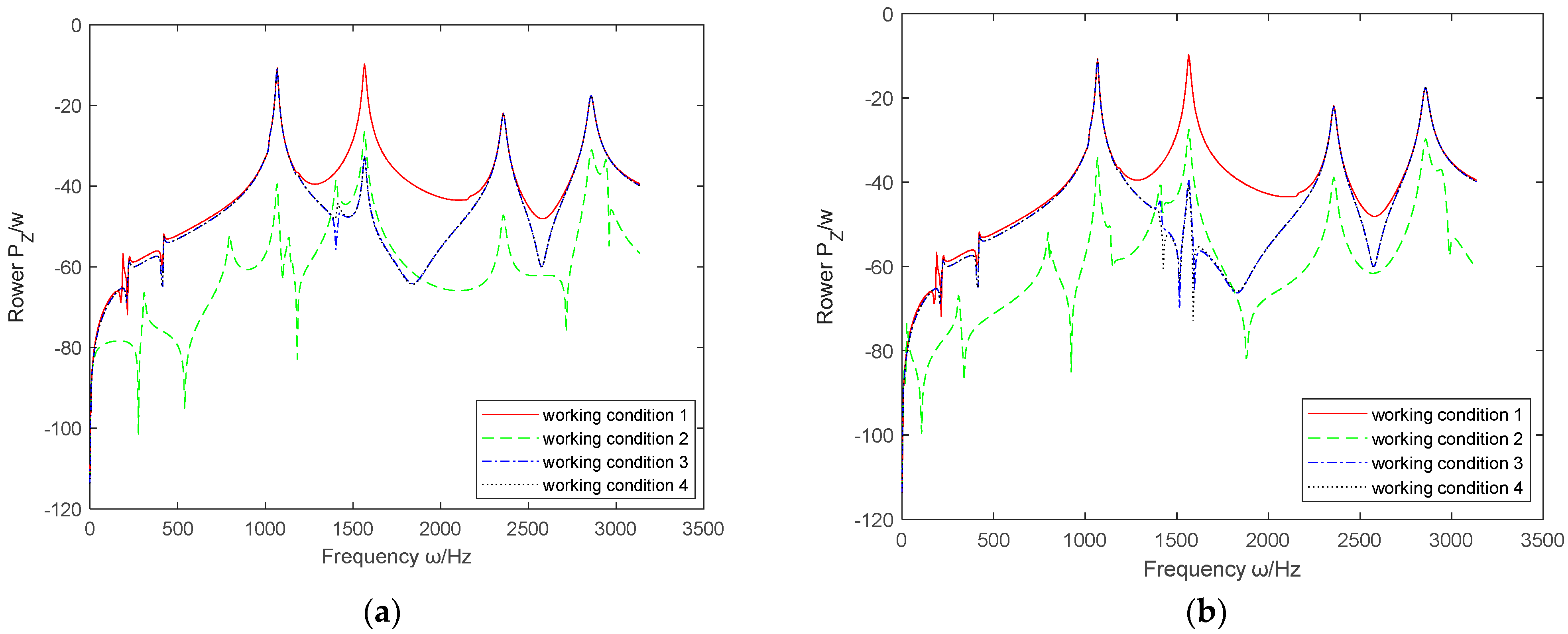
3.3.1. The Influence of Non-Cross Feedback Control Method on the Effectiveness of Active Vibration Control

The controller is the control center of the active actuator, receiving vibration signals collected from sensors and guiding the actuator movement through preset feedback control parameters. Therefore, the above six feedback control parameters are the core parameters of the active control process. This section discusses the use of the single variable principle to simulate and analyze the transmission power flow of a coupled system under the individual action of six feedback control parameters: absolute displacement feedback parameter ${\zeta }_1$, absolute velocity feedback parameter ${\zeta }_2$, absolute acceleration feedback parameter ${\zeta }_3$, relative displacement feedback parameter ${\zeta }_4$, relative velocity feedback parameter ${\zeta }_5$, relative acceleration feedback parameter ${\zeta }_6$.

The vertical axis of the power flow image shown below is the sum of the average excitation power $P_{\mathrm{z}}$ of shell A and shell B, and the horizontal axis is the frequency $\omega$. The four curves in each graph represent:zero feedback, five times feedback $\zeta$, ten times feedback $\zeta$, fifteen times feedback $\zeta$.

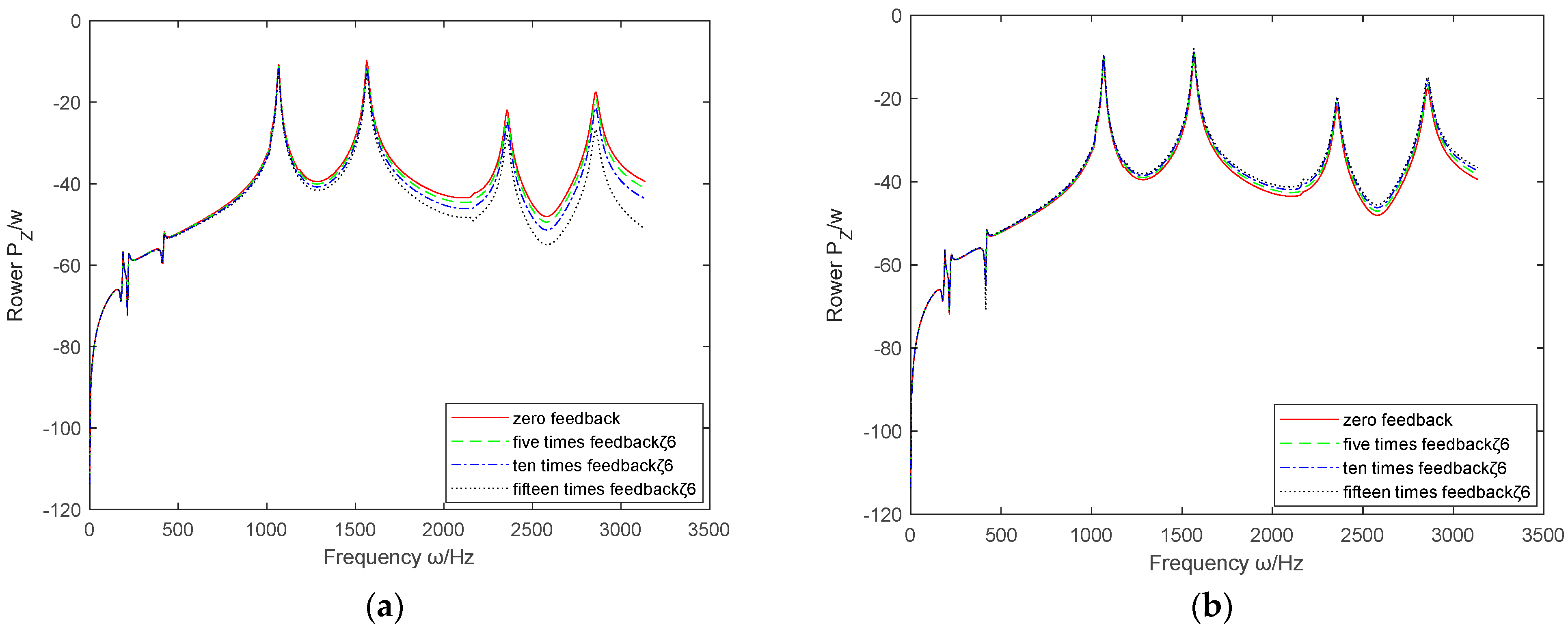
1.

The influence of absolute displacement feedback parameters ${\zeta }_1$

In Figure 3a, as ${\zeta }_1$ increases, the power in the low frequency region gradually decreases, accompanied by a frequency left shift phenomenon, and the power flow image is lower than the initial state. This indicates that the positive controlled gain in this frequency range will increase the energy level of the system, and the improvement effect of vibration control at the resonance peak is good. The larger ${\zeta }_1$, the better the control effect, especially in the low frequency range, where the power flow is significantly lower than that without feedback, and the low frequency control effect is still good.

In Figure 3b, as the absolute value of ${\zeta }_1$ increases, the power flow shows a decreasing trend, accompanied by a frequency shift to the right. This indicates that negative ${\zeta }_1$ can improve the vibration control effect of the system. The resonance peak at 1000 Hz shows an increase in peak value, which may worsen the vibration effect, and the control effect near this range may not be stable.

In summary, the commonality between the two power flow images is that the power flow curve changes significantly in the low frequency range of 0–1000 Hz, while the effects of both are not very obvious in the high frequency range. Combined with the comparison of the image at 2200 Hz, it can be seen that the negative controller gain has a better improvement effect than the positive controller gain. Overall, the control effect of ${\zeta }_1>0$ is relatively more stable.

2.

The influence of absolute velocity feedback parameters ${\zeta }_2$

In Figure 4a, as ${\zeta }_2$ increases, the power flow image decreases significantly, and the control effect becomes better and better. The vibration suppression effect of each resonance peak is also prominent, and the peak value of the resonance peak shows a significant downward trend, with a considerable decrease. The control effect of the last resonance peak in the figure is weak. Overall, when ${\zeta }_2>0$, the low, medium, and high frequency performance of the system has been well improved. In Figure 4b, the changes law of the power flow image with negative value ${\zeta }_2$ is basically consistent with that when ${\zeta }_2>0$.

In summary, regardless of whether ${\zeta }_2$ is positive of negative, and whether the frequency is near the resonance peak or not, its vibration control effect on the entire coupled system is quite significant, and the larger its absolute value, the better the control effect.

3.

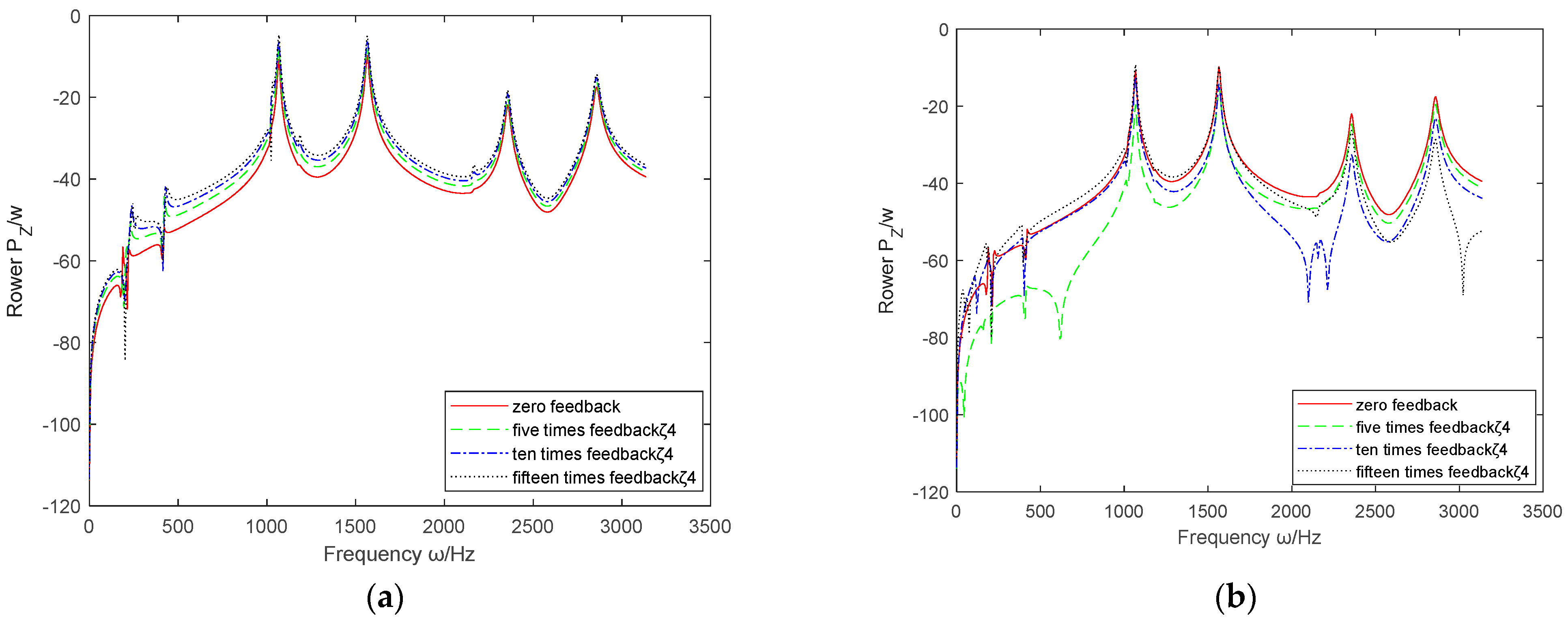
The influence of absolute acceleration feedback parameters ${\zeta }_3$.

In Figure 5a, the power flow curve is basically in a sinking state, with optimization effects almost throughout the entire frequency range. As ${\zeta }_3$ increases, the power decreases, accompanied by a rightward shift in frequency, and the decrease in each resonance peak is significant, indicating good control effect. In Figure 5b, the overall state of the power flow curve is basically consistent with that of ${\zeta }_3>0$.

In summary, ${\zeta }_3$ has a significant vibration control effect on the coupled system at almost all frequencies. At ${\zeta }_3>0$, the vibration control effect at medium and low frequencies is prominent, but the larger the value, the better the effect. The control effect at high frequencies is not as obvious as that at medium and low frequencies, but it is still considered very effective. At ${\zeta }_3<0$, the control effect at medium to high frequencies is similar to the overall pattern when positive values are taken. However, at very low frequencies, there is a situation where the power flow after active vibration control is greater than the zero feedback curve, and the control effect here is deteriorated.

4.

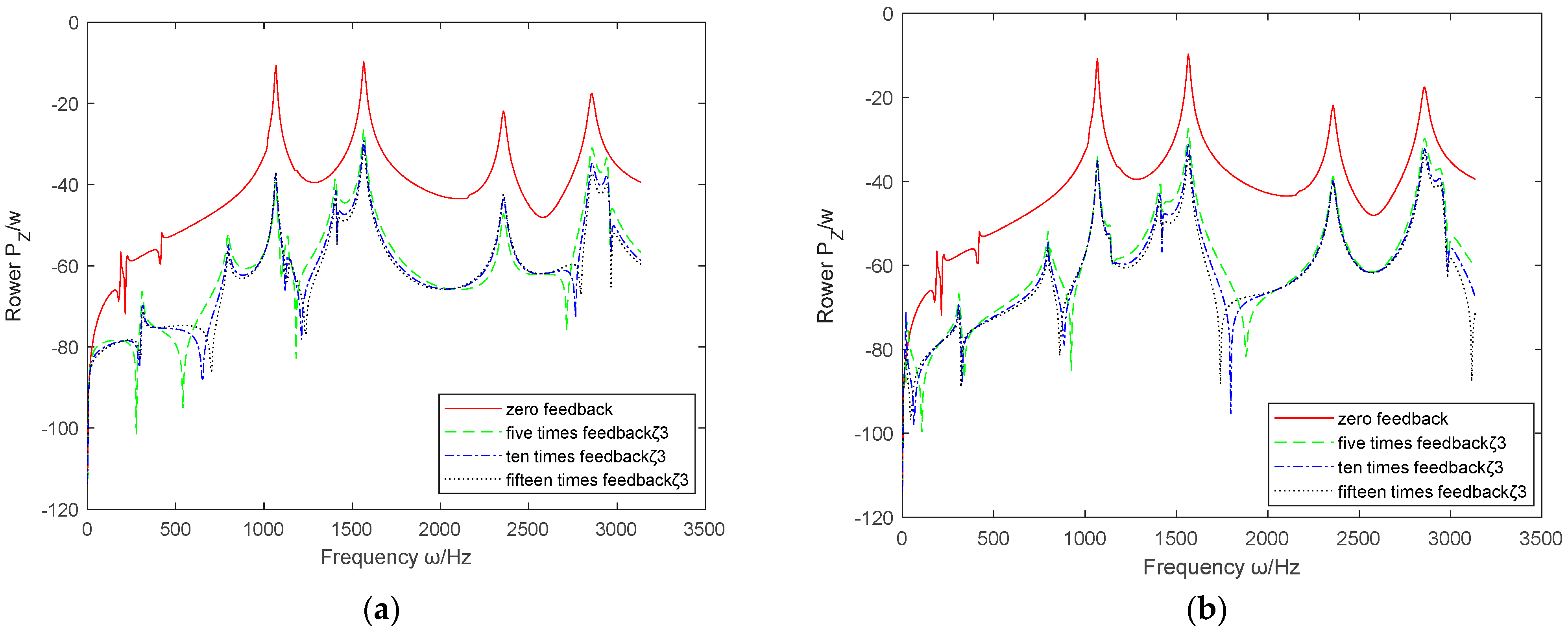
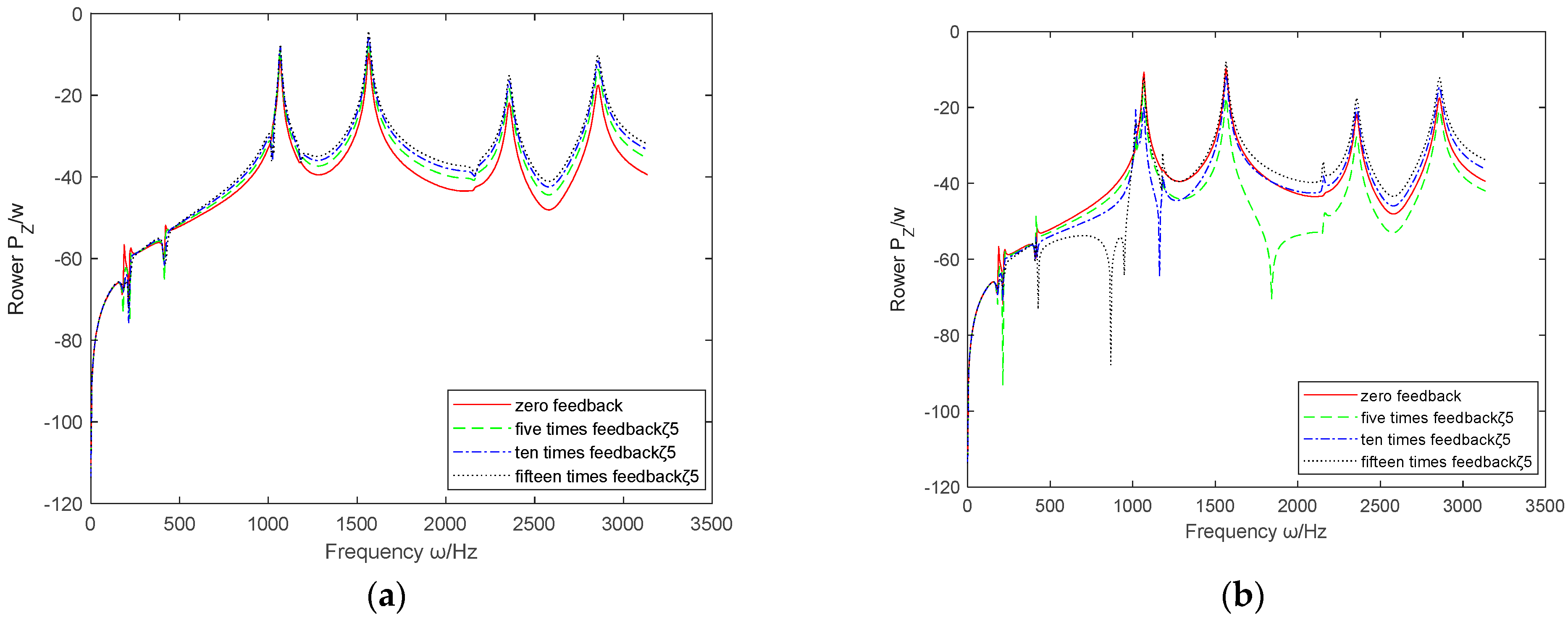
The influence of relative displacement feedback parameters ${\zeta }_4$.

In Figure 6a, when ${\zeta }_4>0$, the power flow curve changes throughout the entire frequency band. By observing the resonance peaks in the graph, it can be seen that the power flow curve with feedback increases compared to zero feedback increases compared to zero feedback, and the larger ${\zeta }_4$, the greater the increase, indicating that the control effect deteriorates when ${\zeta }_4>0$.

In Figure 6b, when ${\zeta }_4<0$, the power flow curve also changes at all frequencies, and the vibration control effect is steadily improved from the resonance peak of 1000–1500 Hz, which basically conforms to the rule that the larger the absolute value of the feedback parameter, the better the control effect. However, in the range of 2000–2500 Hz, as the absolute value of the relative displacement feedback parameter increases, the power flow curve shows a trend of first decreasing and then increasing.

In summary, ${\zeta }_4$ has a certain impact on the vibration control of the coupled system across the entire frequency range. When ${\zeta }_4>0$, the vibration control of each frequency band in the coupled system deteriorates, and the larger its value, the worse the control effect. When ${\zeta }_4<0$, the control effect of mid high frequency vibration is improved, while the improvement of low frequency is not stable, and as ${\zeta }_4$ increases to a certain threshold, the improvement effect may be somewhat suppressed.

5.

The influence of relative velocity feedback parameters ${\zeta }_5$

In Figure 7a, when ${\zeta }_5>0$, the amplitude of the power flow curve change is not very large. Compared to ${\zeta }_2$, the control effect is weaker. In the low frequency range, as ${\zeta }_5$ increases, the power flow gradually decreases, indicating that ${\zeta }_5$ can improve the low frequency vibration control effect of the coupled system. However, as the frequency increases, regardless of whether it is located at the resonance peak or not, its power flow curve is above the non-feedback curve, indicating that in the mid to high frequency range, a positive value of ${\zeta }_5$ does not actually deteriorate the vibration control effect of the coupled system, and the larger the absolute value of ${\zeta }_5$, the greater the degree of deterioration.

In Figure 7b, when ${\zeta }_5<0$, a relatively significant control effect can be observed in the low frequency range, and as the absolute value of ${\zeta }_5$ increases, the power flow shows a significant decrease, indicating that the control effect on the mid low frequency is good when ${\zeta }_5<0$. However, as the frequency increases, the control effect becomes weaker an even deteriorates like ${\zeta }_5>0$.

In summary, regardless of whether ${\zeta }_5$ takes a positive or negative value, there is a significant improvement in the control effect for low frequencies. When ${\zeta }_5$ takes a negative value, the control effect for medium frequencies is also good, but the control effect in the high frequency range is not satisfactory.

6.

The influence of relative acceleration feedback parameters ${\zeta }_6$

In Figure 8a, when ${\zeta }_6>0$, observing the image, the control effect is almost not reflected in the low frequency range. As the frequency increases, the control effect becomes more and more obvious, and there is no frequency shift. As ${\zeta }_6$ increases, the power flow curve shows a downward trend, indicating that the control effect is getting better and better. In Figure 8b, the characteristics of the low frequency band are the same as ${\zeta }_6>0$. As the frequency increases and the absolute value of ${\zeta }_6$ increases, the power flow curve shows an upward trend, indicating that the control effect gradually deteriorates.

In summary, regardless of whether ${\zeta }_6$ is positive or negative, it almost does not affect the control effect in the low frequency range. As the frequency increases, when ${\zeta }_6>0$, the absolute value of ${\zeta }_6$ becomes larger, and the control effect becomes better. When ${\zeta }_6<0$, the larger the absolute value of ${\zeta }_6$, the worse the control effect.

7.

Comparison results of six cases without cross feedback parameters

Based on the single variable rule and the above analysis, the following summary can be made:

(1)

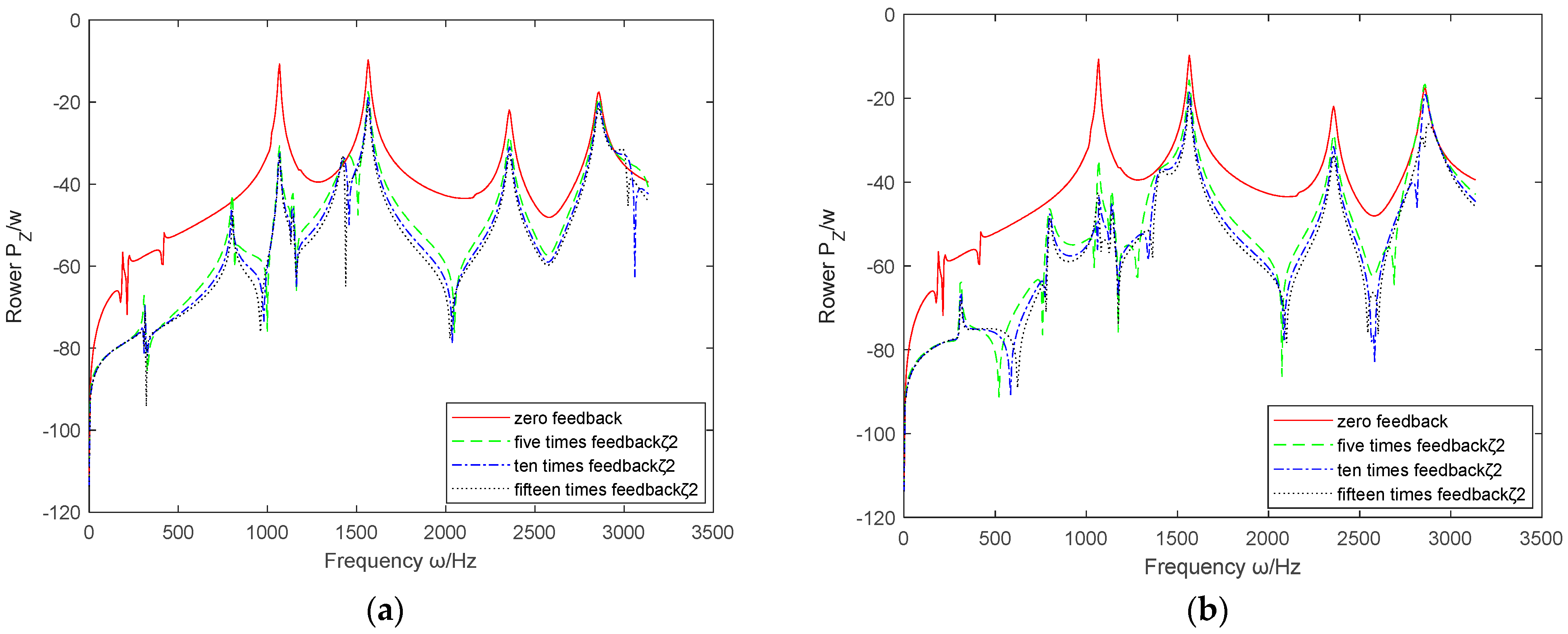
By comparing the absolute and relative feedback parameters of displacement, velocity, and acceleration, it can be concluded that ${\zeta }_1$, ${\zeta }_2$, and ${\zeta }_3$ are generally superior to ${\zeta }_4$, ${\zeta }_5$, and ${\zeta }_6$ in vibration control of the coupled system.

(2)

Based on the above six sets of images, it can be seen that the effective range controlled by ${\zeta }_2$ and ${\zeta }_3$ is the largest, covering the entire working range. The effects of ${\zeta }_5$ and ${\zeta }_6$ are not significant and may even cause deterioration.

(3)

${\zeta }_1$ has improved the active control effect of the coupling system in the middle and low frequencies, but the control effect in the high frequency part is not ideal; on the contrary,${ \zeta }_6$ has almost no control effect at low frequencies, but when it is positive, the control effect in the mid to high frequency range is also improved, although compared to ${\zeta }_2$ and ${\zeta }_3$, the control effect is not as prominent.

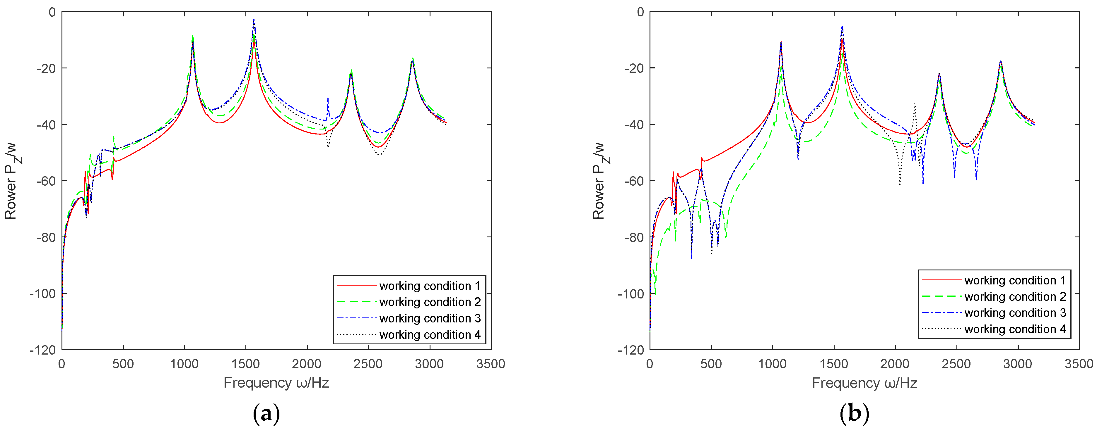
3.3.2. Composite Case Without Cross Feedback Parameters

If two of more of the six feedback parameters mentioned above participate in control at the same time (i.e., not using the single variable principle), the distribution setting is:

Brief analysis of power flow curves for four scenarios: no feedback (${\zeta }_k=0$), single feedback (${\zeta }_i$), single feedback (${\zeta }_j$), and composite feedback (${\zeta }_i$ and ${\zeta }_j$ work together)$(i,j=1,2,3,4,5,6,i\ne j)$.

The feedback parameter values for each individual feedback below are 15 times feedback $\zeta$ (i.e., the fourth curve discussed earlier).

Based on the analysis of the three figures above, it can be seen that in Figure 9, ${\mathit{G}}_1$, ${\mathit{G}}_2$, ${\mathit{G}}_3$ act simultaneously, with ${\mathit{G}}_3$ (i.e., the absolute acceleration feedback parameter ${\zeta }_3$) playing a dominant role. After ${\mathit{G}}_1$, ${\mathit{G}}_2$, ${\mathit{G}}_3$ are added together, further improvement is achieved on the basis of $G_3$ improving the control effect, but it is not very obvious. In Figure 10, when ${\mathit{G}}_4$, ${\mathit{G}}_5$, ${\mathit{G}}_6$ act simultaneously, the final result actually deteriorates the control effect of the system, playing a completely opposite role. Figure 11 further superimposes the above two composite results. Compared to the situation without feedback, the power flow curve shows a decreasing state across the entire frequency band.

The above simple analysis cannot provide an accurate conclusion on the superposition of parameters without cross feedback, as there are too many situations to consider. However, after observation, there are still some gains: In the above discussion, the superposition of ${\mathit{G}}_4$, ${\mathit{G}}_5$, ${\mathit{G}}_6$ actually deteriorates the vibration control of the system, but when the six feedback parameters act simultaneously, the overall control effect is improved. It can be inferred that, assuming all other parameters are consistent, ${\mathit{G}}_1$, ${\mathit{G}}_2$, ${\mathit{G}}_3$ play a dominant role in active vibration control of the coupled system compared to ${\mathit{G}}_4$, ${\mathit{G}}_5$, ${\mathit{G}}_6$; the appropriate values of six parameters can improve the active vibration control effect of the coupled system to a higher level. The specific optimal solution falls within which range, and the optimization discussion is too complex, so this article will not elaborate further.

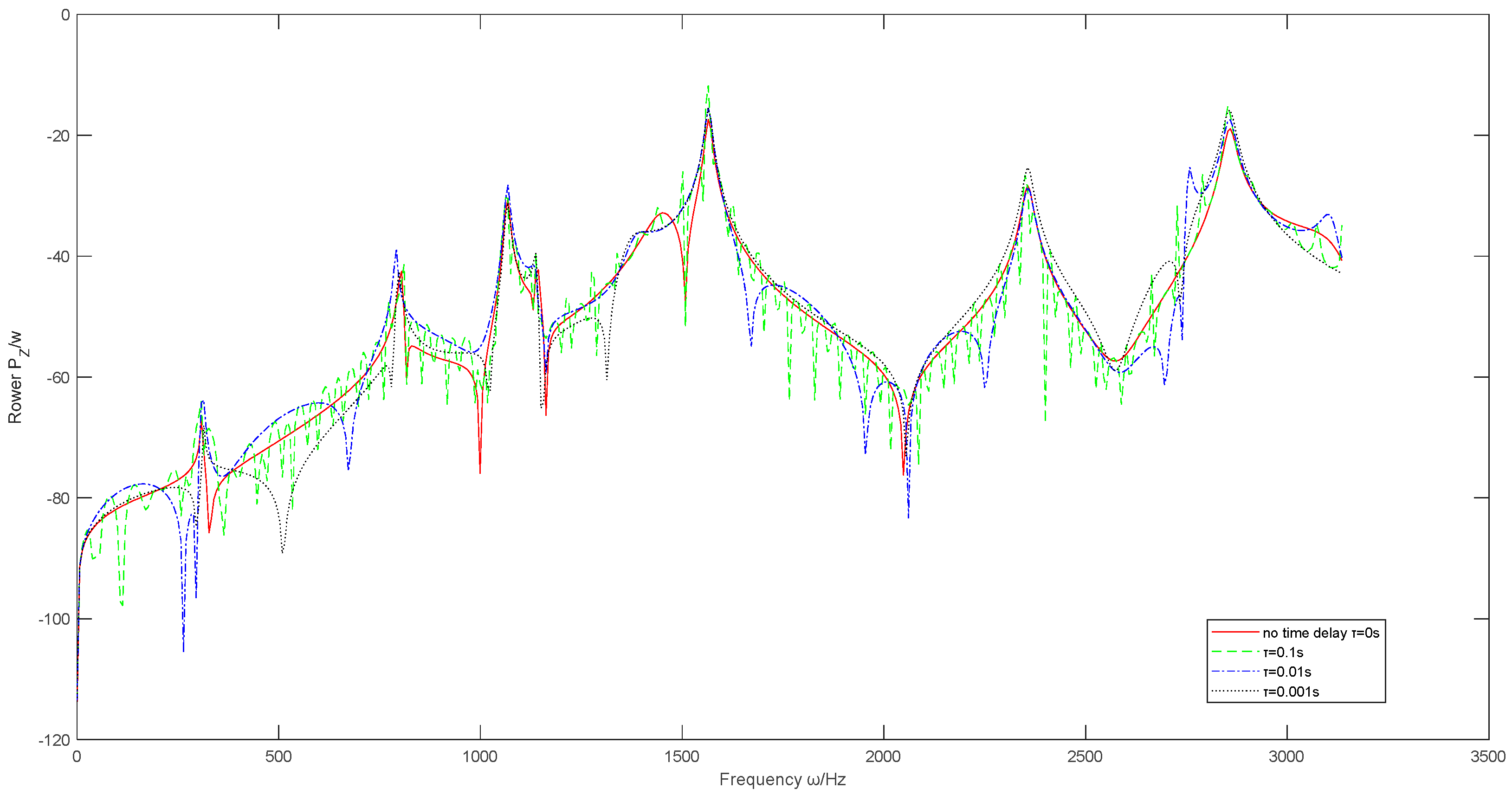
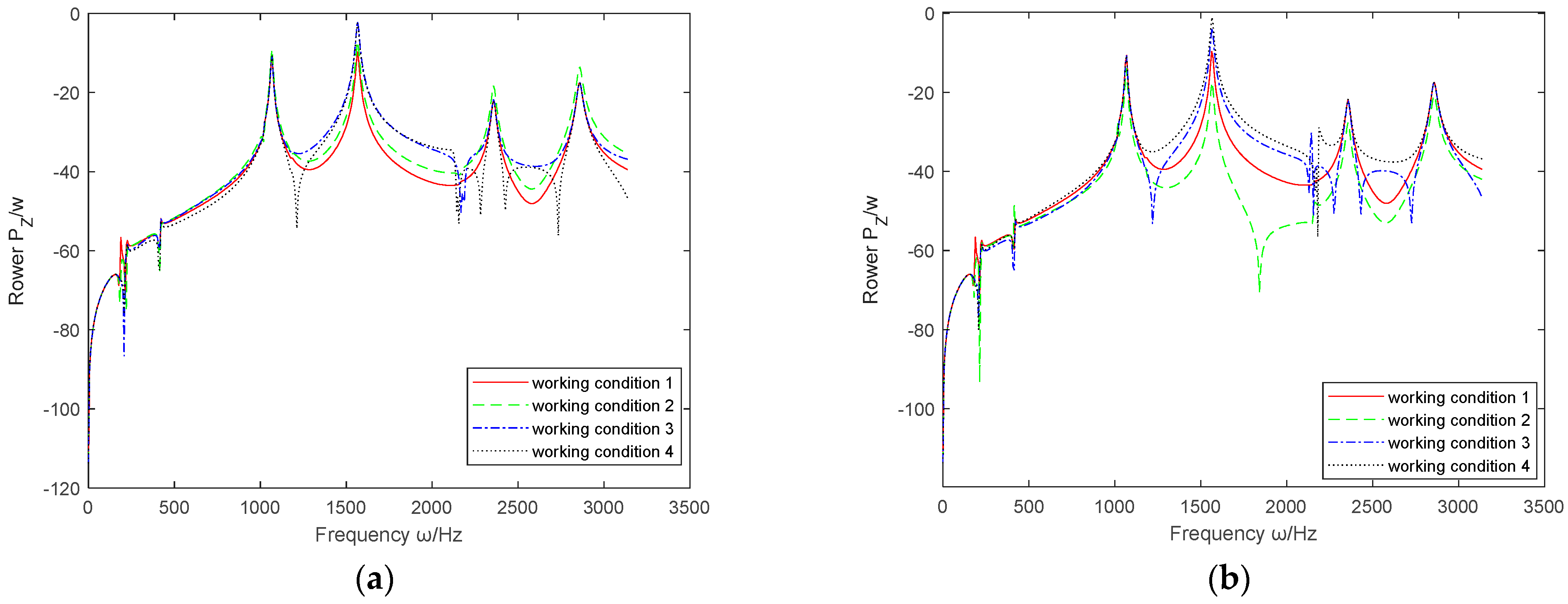
3.3.3. The Influence of Time Delay of Active Actuators on the Effectiveness of Active Vibration Control

In this discussion, ${\zeta }_2$ will be taken as a fixed value except for zero (consistent with the above discussion for ease of comparison), and all other feedback parameters will still use the initial settings to compare the impact of different values of delay compensation ${\tau }^{\prime }$ on the active vibration control effect of the coupled system.

As shown in Figure 12, when ${\tau }^{\prime }=0.001 \mathrm{s}$, the active vibration control effect has been improved in the mid low frequency range (0–1600 Hz), especially at low frequencies, compared to ${\tau }^{\prime }=0.1 \mathrm{s}$, ${\tau }^{\prime }=0.01 \mathrm{s}$, the control effect is more obvious. When ${\tau }^{\prime }=0.1 \mathrm{s}$, the power flow curve fluctuates greatly and is very unstable throughout the entire frequency range, which can deteriorate the vibration control effect. Observing the end of the image, it can be seen that when the frequency reaches a certain level, the four curves basically overlap and move in the same direction, indicating that the effect of delay compensation is not significant in high frequency bands. In summary, the main impact of time delay on coupled systems is to improve the control effect of medium and low frequencies, and has little effect on the vibration control of high frequencies. However, excessive delay compensation ${\tau }^{\prime }$ can make the power flow curve of the coupled system extremely unstable.

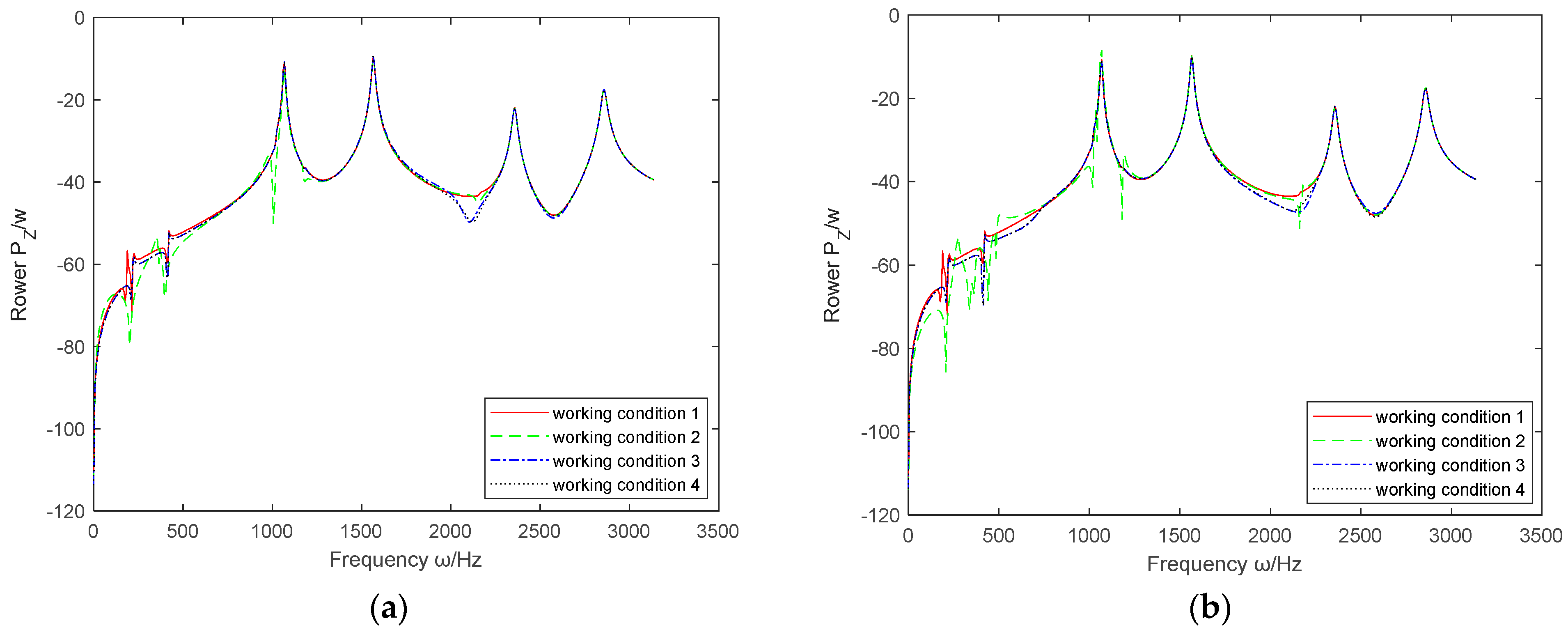
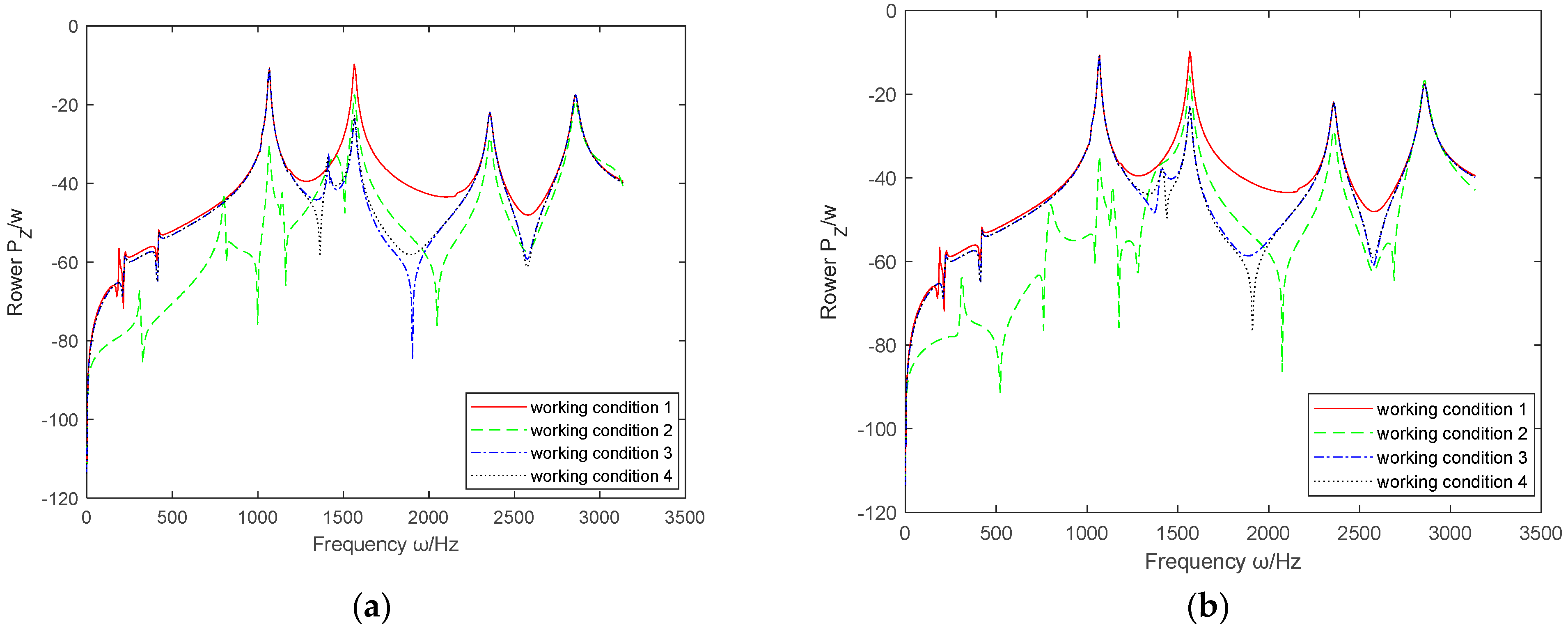
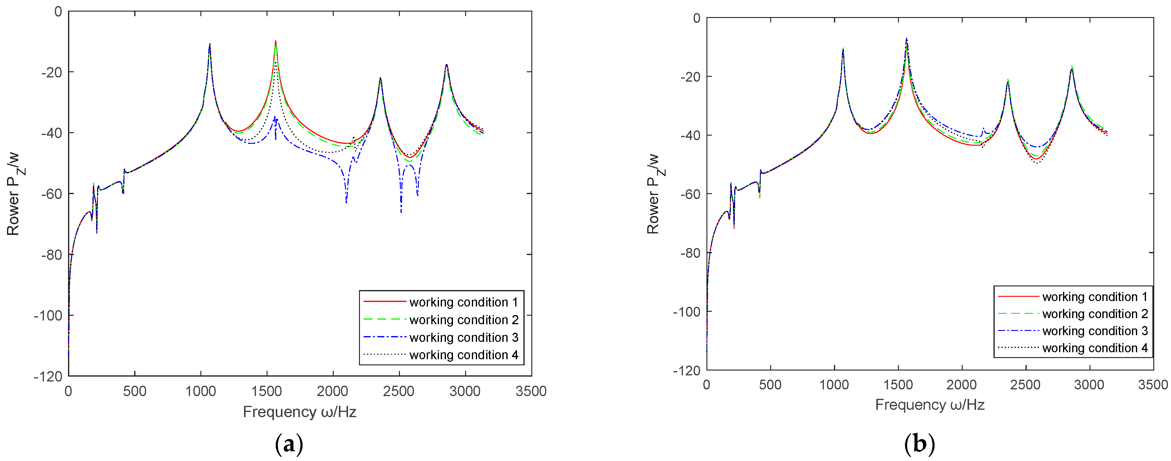
3.3.4. The Influence of Cross Feedback Control Method on the Effectiveness of Active Vibration Control

In addition to receiving sensor signals from its own installation location, the controller can also receive sensor signals from other controller installation locations. Now consider the situation where the active actuator gains relative to the controlled that receives feedback signals from other installation points, which is quite complex.

Similarly, let $K={\displaystyle \raisebox{1ex}{$k_{\mathrm{a}}$}\!\left/ \!\raisebox{-1ex}{$(1+\mathrm{j}{\tau }_{\mathrm{a}}\omega )$}\right.}$, $N=6$, and simplify Equation (15) as

$${\mathit{G}}_k={\displaystyle \frac{K}{R}}·\left[\begin{array}{c}{g}_{11}^{(k)}\\ g_{21}^{(k)}\\ ···\\ g_{61}^{(k)}\end{array}\begin{array}{c}{g}_{12}^{(k)}\\ g_{22}^{(k)}\\ ···\\ g_{62}^{(k)}\end{array}\begin{array}{c}···\\ ···\\ ···\\ ···\end{array}\begin{array}{c}{g}_{16}^{(k)}\\ g_{26}^{(k)}\\ ···\\ g_{66}^{(k)}\end{array}\right]$$

(38)

All sensors, controllers, or actuators are of the same specifications and symmetrically distributed, so the controlled gain of the feedback signal obtained by each active actuator from other actuators is the same. Therefore, $g_{rs}^{\left(k\right)}=g_{11},(r,s=\mathrm{1,2},\mathrm{3,4},\mathrm{5,6})$, and the feedback control parameter matrix $G_k$ is only related to $g_{11}^{(k)}$. The following are defined separately:

Set the situation of a single active vibration control without feedback (i.e., ${\zeta }_k=0$) as working condition 1;

Set the situation of a single active vibration control without cross feedback and time delay as working condition 2;

Set the situation of a single active vibration control with no time delay and cross feedback as working condition 3;

Set the situation of a single active vibration control with time delay and cross feedback as working condition 4;

(Note: Other basic parameters of the coupled system still use the initial settings.)

1. The influence of absolute displacement feedback parameters ${\zeta }_1$ (the absolute values of the two parameters are equal).

In Figure 13, the difference between the laws of ${\zeta }_1>0$ and ${\zeta }_1<0$ is not significant. In the large range of medium and high frequencies, regardless of whether there is cross feedback, the control effect is not obvious. From the power fluctuation around 2000 Hz, it can be seen that the control effect with cross feedback is obviously much better than that without cross feedback. In the low frequency range, it can be observed that the swing amplitude of the power flow curve without cross feedback (working condition 2) is large, and its control effect is not very stable. However, the power flow curve with cross feedback (working condition 3), although the decrease in amplitude is not significant compared to the curve without feedback, is very stable. By comparing the two cases with and without time delay and cross feedback, it is found that the effect of delay compensation on vibration control is not significant.

2. The influence of absolute velocity feedback parameters ${\zeta }_2$ (the absolute values of the two parameters are equal)

In Figure 14, when ${\zeta }_2>0$, overall, the control effect of cross feedback on the resonance peak is not ideal, while the control effect of low frequency without cross feedback is better, and the control effect of medium high frequency with cross feedback is better. In addition, regardless of whether there is crossover, the overall vibration control effect is very good, and due to the presence of time delay ${\tau }^{\prime }$, the further strengthened control effect makes the power flow curve around 2000 Hz smoother and more stable. When ${\zeta }_2<0$, the change pattern is basically the same as when ${\zeta }_2>0$, and the existence of time delay ${\tau }^{\prime }$ makes the strengthening of control effect more obvious.

3. The influence of absolute acceleration feedback parameters ${\zeta }_3$ (the absolute values of the two parameters are equal)

In Figure 15, regardless of whether ${\zeta }_3$ is positive or negative, there is not much difference in the image, and the overall pattern is the same as ${\zeta }_2$. The impact of time delay ${\tau }^{\prime }$ is not significant, so it will not be repeated.

4. The influence of relative displacement feedback parameters ${\zeta }_4$ (the absolute values of the two parameters are equal)

In Figure 16a, when ${\zeta }_4>0$, according to the discussion in Figure 6a, it will deteriorate the vibration control effect of the coupled system. An additional finding is that considering the presence of cross feedback further deteriorates the control effect. After considering the time delay, the degree of deterioration of the control effect is relatively alleviated, but the power flow curve is still mostly above the non-feedback curve.

In Figure 16b, when ${\zeta }_4<0$, observing the power flow curve with cross feedback, it was found that the control effect at the resonance peak was almost negligible. At other positions, the control effect with cross feedback was not very prominent, and even in most of the low frequency range, the control effect without cross feedback was still good. The time delay had little effect, and only improved the control effect around 2000 Hz.

5. The influence of relative velocity feedback parameters ${\zeta }_5$ (the absolute values of the two parameters are equal)

In Figure 17a, when ${\zeta }_5>0$, according to Figure 7a, the control effect of the system will deteriorate. Considering the presence of crossover, the control effect of the system will be improved in the low-frequency range, and the degree of improvement will be better than that without crossover; In the mid to high frequency range, except for the resonance peak at 1500 Hz, the presence of cross feedback at other resonance peaks can suppress the deterioration of non-cross feedback. The existence of time delay will further reduce power in certain frequency bands in the mid to high frequency range, playing a certain improvement role. Overall, the control effect is not stable.

In Figure 17b, when ${\zeta }_5<0$, in the low frequency region, for the same ${\zeta }_5$, the control effect with crossover is better than without crossover. However, as the frequency increases, the control effect of the system deteriorates with crossover feedback, and the power fluctuation of the part that improves it is large. Considering the time delay, it will further deteriorate the control effect. Overall, the control effect of cross feedback in medium and high frequencies is also unstable, and regardless of whether time delay ${\tau }^{\prime }$ is considered, its control effect is not ideal, and even counterproductive.

6. The influence of relative acceleration feedback parameters ${\zeta }_6$ (the absolute values of the two parameters are equal)

Regardless of whether ${\zeta }_6$ is positive or negative, whether there is crossover, or whether there is time delay, low frequency vibration control does not work as the frequency increases. Observing Figure 18a, the presence of cross feedback (working condition 3) further improves the control effect of the system compared to the absence of cross feedback (working condition 2), but considering time delay actually suppresses the control effect with cross feedback. However, it still has an improvement effect, and the power flow curve is smoother. Observing Figure 18b, the presence of cross feedback (working condition 3) further deteriorates the control performance of the system compared to the absence of cross feedback (working condition 2). However, when considering time delay ${\tau }^{\prime }$, it actually mitigates the degree of deterioration. At the position of 2500 Hz, time delay ${\tau }^{\prime }$ even has an improvement effect.

4. Conclusions

This article studies and analyzes a method of active feedback control by inserting active supports between double-layer cylindrical shells, with the aim of improving the low frequency vibration control effect. As a theoretical study, this article adopts an analytical dynamics modeling method, which considers complex factors such as arbitrary number of supports, installation position and direction, absolute displacement, velocity, acceleration feedback control, relative displacement, velocity, acceleration feedback control, and time delay. Regarding the composite situation without cross feedback parameters, the specific optimal solution falls within which range. The optimization discussion is complex, but it also has certain discussion value and can be used as a future research point. The various situations discussed above are summarized into a table in Appendix C for easy viewing.

Based on a simulation example with six supports, the following conclusions can be drawn:

(1)

In the non-cross feedback control method, the absolute feedback parameter has a better overall vibration control effect on the coupled system than the relative feedback parameter. In addition, the absolute velocity and acceleration feedback parameters have the largest effective range and the most obvious effect on improving vibration control. Compared with the vibration control effect of the relative velocity and acceleration feedback process, the power flow curve is smoother and more stable. The absolute displacement feedback parameter improves the control effect of the coupling system’s mid low frequency vibration, while the control effect of the high frequency part is no ideal. However, when the controlled gain is positive, the relative acceleration feedback parameter improves the control effect in the mid high frequency.

(2)

In the non-cross feedback control method, the relative displacement and velocity feedback control when the controlled gain is positive, as well as the relative acceleration feedback control when the controlled gain is negative, have a deteriorating effect on the control performance of the system. Thus, for absolute feedback control parameters, the control effect of relative feedback control parameters is unstable, and if the controlled gain is not selected appropriately, it will have the opposite effect.

(3)

In the non-cross feedback control method, except for the relative acceleration feedback control parameter, all other feedback parameters have a certain low frequency control effect, especially the control effect of the three absolute feedback control parameters is the most prominent. If the influence of time delay is considered, the low frequency control effect will be more obvious.

(4)

Appropriately increasing the delay compensation ${\tau }^{\prime }$ of the active actuator can improve the mid low frequency control effect of the coupled system, but it has little impact on the high frequency region, and excessive delay compensation ${\tau }^{\prime }$ can make the power flow curve of the coupled system extremely unstable.

(5)

When the absolute displacement feedback parameter is applied, considering factors such as cross feedback control and time delay, the difference in its image is not significant. According to (1), the working range of absolute velocity and acceleration feedback control is very wide, but considering the cross feedback control method, its improvement degree is suppressed over a large area. The relative acceleration feedback parameter has little effect at low frequencies, regardless of whether cross feedback or time delay is considered. However, at medium to high frequencies, cross feedback control enhances the effect of no cross feedback, while time delay suppresses the effect of cross feedback control. Among the three relative feedback control parameters, the role of the cross feedback control method is actually to amplify the vibration control effect of the non-cross feedback control method, whether this effect is improved or deteriorated.

References

- Zhang, L.; Zhao, L.; Pan, L. Research progress of composite cylindrical shells. Polym. Compos. 2023, 44, 7298–7316. [Google Scholar] [CrossRef]
- Zhang, D.; Chen, H.; Li, P. Axisymmetric finite element boundary element coupling calculation method for vibration of cylindrical shells with sealing plates in dynamic water. J. Vib. Eng. 2025, 38, 687–696. [Google Scholar]
- Nie, L. Study on the buckling behavior of double-layer cylindrical shells under uniform axial compression. Jiangsu Univ. Sci. Technol. 2023. [Google Scholar]
- Liu, W.; Pang, L.; Lv, Z. Free Vibration Analysis of Functionally Graded Piezoelectric Porous Microcylinder Shell with Elastic Support. J. Appl. Mech. 2024, 41, 411–421. [Google Scholar]
- Wang, T.; Tan, D.; Hou, Y. Analytical and experimental investigation of vibration response for the cracked fluid-filled thin cylindrical shell under transport condition. Appl. Math. Model. 2025, 142, 115969. [Google Scholar] [CrossRef]
- Liu, X.; Sun, W.; Liu, H. An investigation of vibration responses for bolted composite flanged-cylindrical shells considering material and joint nonlinearity. Thin Walled Struct. 2024, 204, 112335. [Google Scholar] [CrossRef]
- Zhou, Y.; Sun, X.; Kong, J. Preparation process and vibration characteristics analysis of composite cylindrical shell with co cured damping film embedded. J. Weapon Equip. Eng. 2024, 45, 254–261. [Google Scholar]
- Lv, Z.; Liu, W.; Liu, C. The influence of thermal environment on the modal frequency of functionally graded thin-walled cylindrical shells. Noise Vib. Control. 2022, 42, 28–33. [Google Scholar]
- Hu, Z.; Li, S.; Liu, Z. Analysis of Bearing Capacity and Explosion Resistance of Double layer Pressure resistant Reinforced Cylindrical Shell Structure. Chin. Ship Res. 2024, 19, 205–216. [Google Scholar]
- Tang, Q.; Li, B.; Ding, Z. Optimization of buckling bearing capacity of sandwich cylindrical shell structure under axial compression load. Mech. Des. Manuf. 2020, 80–84. [Google Scholar]
- Li, S.; Zhu, S.; He, W. Optimization design characteristics analysis of titanium alloy double-layer reinforced cylindrical shell under different design requirements. Chin. Ship Res. 2025, 20, 317–328. [Google Scholar] [CrossRef]
- Liu, S.; Huo, R.; Wang, L. Vibroacoustic Transfer Characteristics of Underwater Cylindrical Shells Containing Complex Internal Elastic Coupled Systems. Appl. Sci. 2023, 13, 3994. [Google Scholar] [CrossRef]
- Wang, L.; Huo, R. Effect of Support Stiffness Nonlinearity on the Low-Frequency Vibro-Acoustic Characteristics for a Mechanical. Inventions 2023, 8, 118. [Google Scholar] [CrossRef]
- Wang, R.; Huang, J. Research on the Relationship between Structural Parameters and Instability Modes of Ring Ribbed Cylindrical Shells. Equip. Environ. Eng. 2025, 22, 77–86. [Google Scholar]
- Liu, W.; Wang, X.; Tang, Y. Research on the control effect of irregular spacing between large ribs on vibration transmission of cylindrical shells. Ship Sci. Technol. 2023, 45, 7–13. [Google Scholar]
- Liu, J.; Li, S. Research on Vibration Characteristics of Viscoelastic Damping Cylindrical Shell Based on GHM Model. Dalian Univ. Technol. 2021, 931–943. [Google Scholar] [CrossRef]
- Zhang, J. Optimization analysis of cylindrical shell vibration control based on dynamic absorbe. Key Laboratory of Ship Vibration and Noise, Hubei Acoustic Society. In Proceedings of the 2016 Acoustic Technology Academic Conference China Shipbuilding Research and Design Center, Key Laboratory of Ship Vibration and Noise, Wuhan, China, October 2016; pp. 26–29. [Google Scholar]
- Wang, L.; Huo, R.; Liu, S.; Li, Y.; He, D. Average Energy Transfer Characteristics and Control Strategy of Active Feedback Sound Insulation for Water-Filled Acoustic System Based on Double-layer Piate Structure. Appl. Sci. 2022, 12, 11482. [Google Scholar] [CrossRef]
- Li, X. Research on piezoelectric energy harvesting and active vibration control of cylindrical shells. Master’s Thesis, Zhejiang University, Hangzhou, China, 2012. [Google Scholar]
- Geng, X.; Yin, S.; Zhou, J. Optimization method for active control actuator position of cylindrical shell vibration. J. Underw. Unmanned Syst. 2020, 28, 650–656. [Google Scholar]
- Liu, T.; Wang, C.; Liu, Q. Dynamics and Active Vibration Control Analysis of Piezoelectric Functionally Graded Plates Based on Isogeometric Method. Eng. Mech. 2020, 37, 228–242. [Google Scholar]
- Tang, B.; Li, Y.; Zhang, Z. Research progress on vibration and sound radiation problems of composite multi-layer cylindrical shells. Mater. Introd. 2023, 37, 256–263. [Google Scholar]
- Wang, F.; He, L.; Weng, Z. Modeling of underwater vibration of double-layer ribbed cylindrical shell based on neural network. China Shipbuilding Engineering Society, Key Laboratory of Ship Vibration and Noise. In Proceedings of the 15th Symposium on Underwater Noise of Ships Key Laboratory of Ship Vibration and Noise, Zhengzhou, China, 1 August 2015; pp. 123–129. [Google Scholar]
- Chai, K.; Liu, J.; Lou, J. Vibration characteristics of cylindrical shells with discontinuous connections based on the spectral element method. Int. J. Solids Struct. 2025, 308, 113148. [Google Scholar] [CrossRef]
- Wu, J.; Yan, B.; Wu, W. Vibration Characteristics Analysis of Ribbed Cylindrical Shell Based on Spectral Element Method. China Shipbuild. 2025, 1–11. Available online: http://kns.cnki.net/kcms/detail/31.1497.U.20250217.1616.002.html (accessed on 18 February 2025).
- Xu, Z. Elasticity; Higher Education Press: Beijing, China, 2016; pp. 28–33. [Google Scholar]
- Yu, A.; Zhao, Y.; Hou, J. Study on Vibration Transmission Characteristics of Double layered Shells with Elastic Connections and Interlayer Fluid. Vib. Shock 2023, 42, 167–176+205. [Google Scholar] [CrossRef]