
Technical–Economic Assessment and FP2O Technical–Economic Resilience Analysis of the Gas Oil Hydrocracking Process at Large Scale


Abstract
1. Introduction
2. Materials and Methods
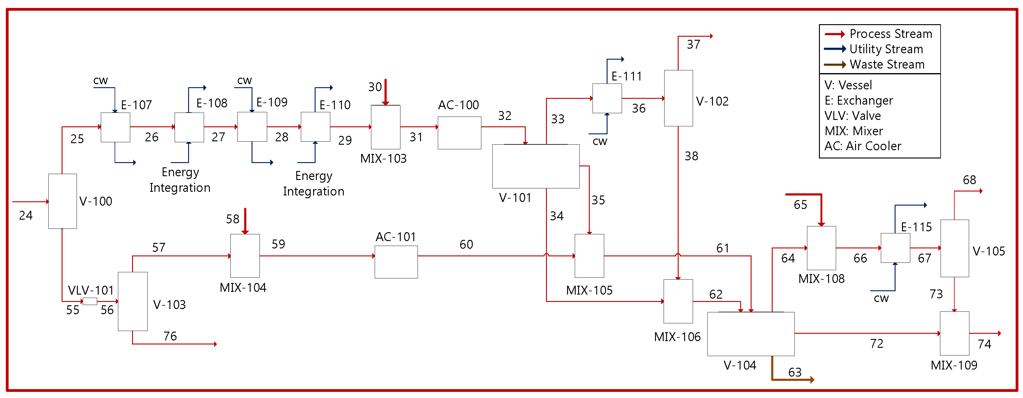
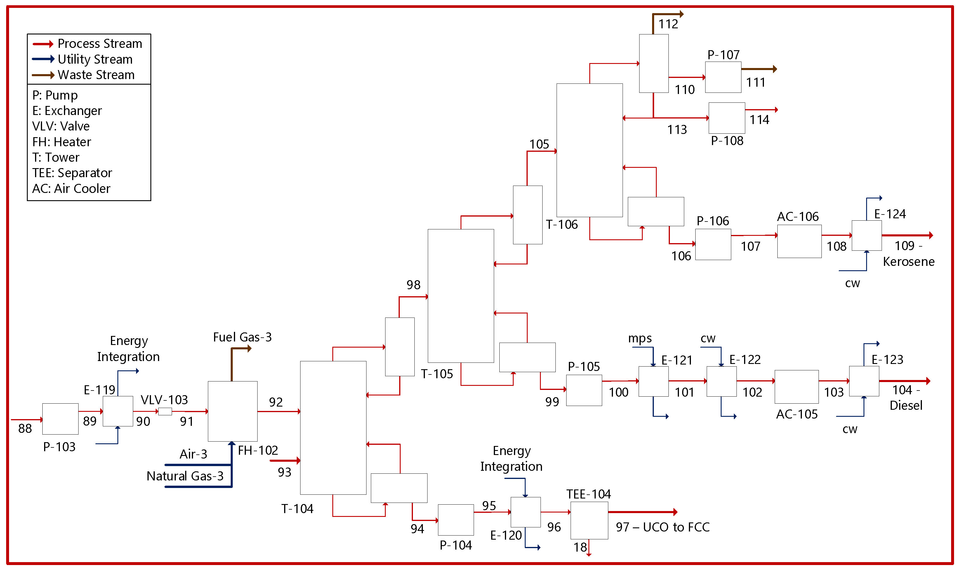
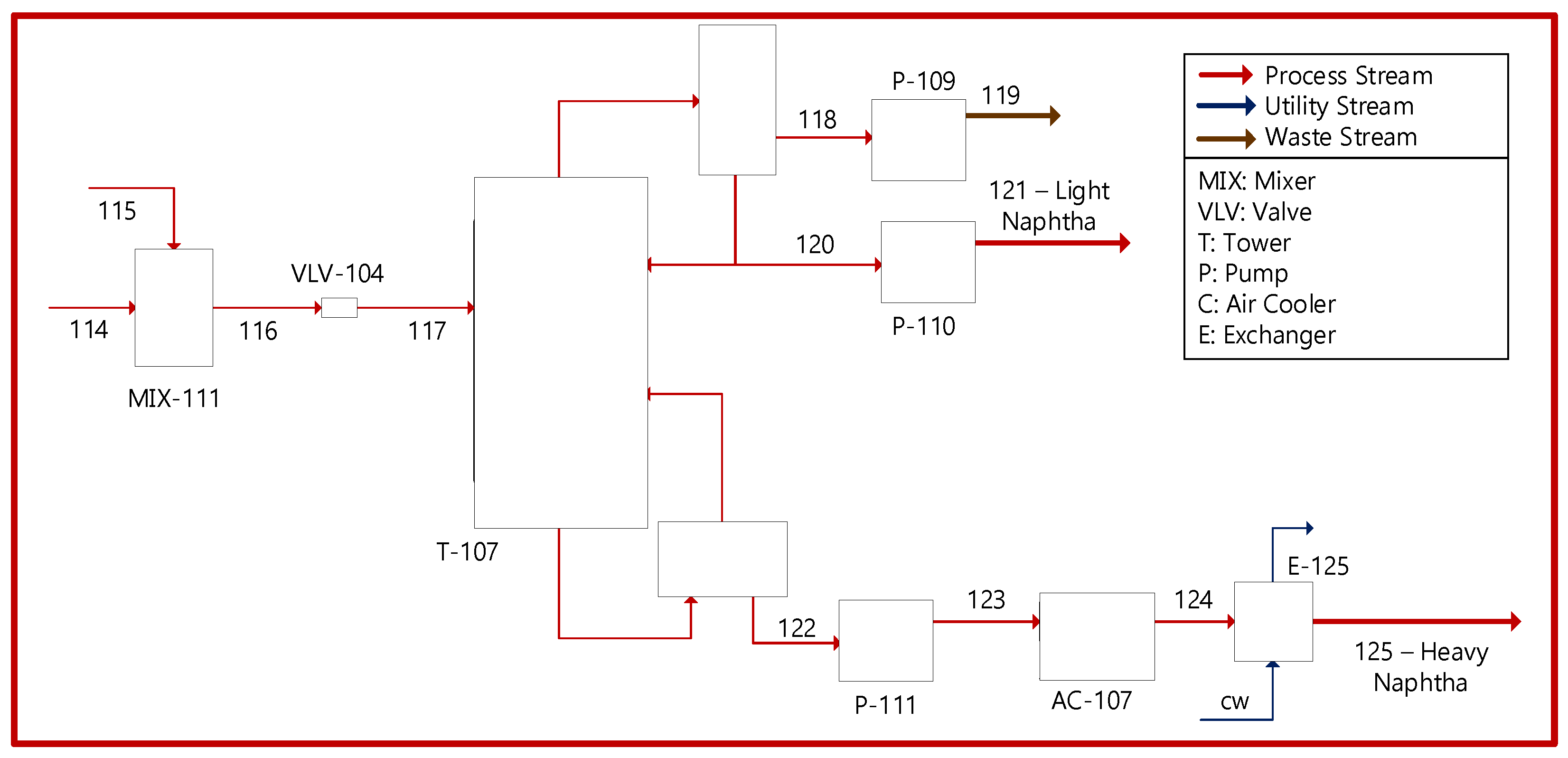
2.1. Process Description
2.2. Technical–Economic Evaluation
2.3. Technical–Economic Resilience Analysis via FP2O Methodology
3. Results and Discussion
3.1. Technical–Economic Evaluation Analysis
3.2. FP2O Technical–Economic Resilience Analysis
4. Conclusions
Author Contributions
Funding
Institutional Review Board Statement
Informed Consent Statement
Data Availability Statement
Acknowledgments
Conflicts of Interest
Abbreviations
| ACR | Annual Cost/Revenue |
| AFCs | Annualized Fixed Costs |
| AOCs | Annualized Operating Costs |
| BEP | Break-Even Point |
| CCF | Cumulative Cash Flow |
| DA | Depreciation and Amortization |
| DFCI | Direct Fixed Capital Investment |
| DGP | Depreciable Gross Profit |
| DPBP | Depreciable Payback Period |
| DPCs | Direct Production Costs |
| EBIT | Earnings Before Interest, and Taxes |
| EBITDA | Earnings Before Interest, Taxes, Depreciation, and Amortization |
| EBT | Earnings Before Taxes |
| ECI | Equipment Cost Index |
| EFB | Empty Fruit Bunches |
| EP1 | Economic Potential 1 |
| EP2 | Economic Potential 2 |
| EP3 | Economic Potential 3 |
| FCC | Fluidized Catalytic Cracking |
| FCHs | Fixed Charges |
| FCI | Fixed Capital Investment |
| FOB | Free on Board |
| FP2O | Feedstock–Product–Process–Operating |
| GEs | General Expenses |
| GP | Gross Profit |
| HKGO | Heavy Gas Oil |
| IFCI | Indirect Fixed Capital Investment |
| IRR | Internal Rate of Return |
| LCO | Light Cycle Oil |
| LPG | Liquefied Petroleum Gas |
| M&S | Marshall and Swift |
| MVGO | Medium Vacuum Gas Oil |
| MR | Maintenance and Repairs |
| NAOCs | Normalized Annualized Operating Costs |
| NPV | Net Present Value |
| NVOCs | Normalized Variable Operating Costs |
| OCs | Operating Costs |
| OL | Operating Labor |
| PAT | Profitability After Tax |
| PBP | Payback Period |
| POH | Plant Overhead |
| PSA | Pressure Swing Adsorption |
| PVC | Polyvinyl Chloride |
| ROI | Return On Investment |
| SUC | Start-Up Costs |
| TCI | Total Capital Investment |
| TMC | Total Manufacturing Cost |
| TPC | Total Product Cost |
| U | Utilities |
| UCO | Unconverted Oil |
| VCM | Vinyl Chloride Monomer |
| WCI | Working Capital Investment |
References
- Favennec, J.-P. The Palgrave Handbook of International Energy Economics; Springer: Berlin/Heidelberg, Germany, 2022. [Google Scholar]
- Tirado, A.; Félix, G.; Trejo, F.; Varfolomeev, M.A.; Yuan, C.; Nurgaliev, D.K.; Sámano, V.; Ancheyta, J. Properties of Heavy and Extra-Heavy Crude Oils. In Catalytic In-Situ Upgrading of Heavy and Extra-Heavy Crude Oils; John Wiley and Sons Ltd.: Hoboken, NJ, USA, 2023; pp. 1–38. [Google Scholar]
- Sahu, R.; Song, B.J.; Im, J.S.; Jeon, Y.P.; Lee, C.W. A review of recent advances in catalytic hydrocracking of heavy residues. J. Ind. Eng. Chem. 2015, 27, 12–24. [Google Scholar] [CrossRef]
- Tirado, A.; Félix, G.; Varfolomeev, M.A.; Ancheyta, J. Effect of feedstock properties on the kinetics of hydrocracking of heavy oils. Geoenergy Sci. Eng. 2024, 233, 212603. [Google Scholar] [CrossRef]
- Pham, H.H.; Kim, K.H.; Go, K.S.; Nho, N.S.; Kim, W.; Kwon, E.H.; Jung, R.H.; Lim, Y.-i.; Lim, S.H.; Pham, D.A. Hydrocracking and hydrotreating reaction kinetics of heavy oil in CSTR using a dispersed catalyst. J. Pet. Sci. Eng. 2021, 197, 107997. [Google Scholar] [CrossRef]
- Choudhary, N.; Saraf, D.N. Hydrocracking: A Review. Ind. Eng. Chem. Prod. Res. Dev. 1975, 14, 74–83. [Google Scholar] [CrossRef]
- Mohanty, S.; Kunzru, D.; Saraf, D.N. Hydrocracking: A review. Fuel 1990, 69, 1467–1473. [Google Scholar] [CrossRef]
- Stratiev, D.; Toteva, V.; Shishkova, I.; Nenov, S.; Pilev, D.; Atanassov, K.; Bureva, V.; Vasilev, S.; Stratiev, D.D. Industrial Investigation of the Combined Action of Vacuum Residue Hydrocracking and Vacuum Gas Oil Catalytic Cracking While Processing Different Feeds and Operating under Distinct Conditions. Processes 2023, 11, 3174. [Google Scholar] [CrossRef]
- Novia, N.; Eko Pratama, M.G.; Qodri, R.; Hasanudin, H.; Fudholi, A. Computational fluid dynamics modeling of crude palm oil hydrocracking in fixed-bed reactor. Int. J. Hydrogen Energy 2024, 56, 903–911. [Google Scholar] [CrossRef]
- Marcilly, C. Acido-Basic Catalysis: Application to Refining and Petrochemistry; Editions Technip: Paris, France, 2006; Volume 2. [Google Scholar]
- Valavarasu, G.; Bhaskar, M.; Balaraman, K.S. Mild hydrocracking—A review of the process, catalysts, reactions, kinetics, and advantages. Pet. Sci. Technol. 2003, 21, 1185–1205. [Google Scholar] [CrossRef]
- Robinson, P.R.; Dolbear, G.E. Hydrotreating and Hydrocracking: Fundamentals. In Practical Advances in Petroleum Processing; Springer: New York, NY, USA, 2007; pp. 177–218. [Google Scholar]
- Sotelo, D.S. Beneficios del Proceso de Hidrotratamientos de Gasóleos de Carga a FCC. Rev. Del Cent. De Investig. Univ. La Salle 2000, 4, 37–46. [Google Scholar]
- Herrera-Rodríguez, T.C.; Ramos-Olmos, M.; González-Delgado, Á.D. A joint economic evaluation and FP2O techno-economic resilience approach for evaluation of suspension PVC production. Results Eng. 2024, 24, 103069. [Google Scholar] [CrossRef]
- Tesfaye, T.; Ayele, M.; Ferede, E.; Gibril, M.; Kong, F.; Sithole, B. A techno-economic feasibility of a process for extraction of starch from waste avocado seeds. Clean Technol. Env. Policy 2021, 23, 581–595. [Google Scholar] [CrossRef]
- González-Delgado, Á.D.; Vargas-Mira, A.; Zuluaga-García, C. Economic Evaluation and Technoeconomic Resilience Analysis of Two Routes for Hydrogen Production via Indirect Gasification in North Colombia. Sustainability 2023, 15, 16371. [Google Scholar] [CrossRef]
- García-Maza, S.; González-Delgado, Á.D. Robust simulation and technical evaluation of large-scale gas oil hydrocracking process via extended water-energy-product (E-WEP) analysis. Digit. Chem. Eng. 2024, 13, 100193. [Google Scholar] [CrossRef]
- Bandyopadhyay, R.; Upadhyayula, S. Thermodynamic analysis of diesel hydrotreating reactions. Fuel 2018, 214, 314–321. [Google Scholar] [CrossRef]
- Alsahhaf, T.A.; Elkilani, A.; Fahim, M.A. Fundamentals of Petroleum Refining; Elsevier: Amsterdam, The Netherlands, 2010; Volume 51, p. 81. [Google Scholar]
- Peters, M.S.; Timmerhaus, K.D. Plant Design and Economics for Chemical Engineers; McGraw-Hill Education: New York, NY, USA, 1991. [Google Scholar]
- El-Halwagi, M.M. Overview of Process Economics. In Sustainable Design Through Process Integration; Elsevier: Amsterdam, The Netherlands, 2017; pp. 15–71. [Google Scholar]
- El-Halwagi, M.M. A return on investment metric for incorporating sustainability in process integration and improvement projects. Clean Technol. Environ. Policy 2017, 19, 611–617. [Google Scholar] [CrossRef]
- El-Halwagi, M.M. Sustainable Design Through Process Integration Fundamentals and Applications to Industrial Pollution Prevention, Resource Conservation, and Profitability Enhancement, 2nd ed.; Butterworth-Heinemann: Oxford, UK, 2017. [Google Scholar]
- Arrieta Chacón, S.M. Análisis de Costos Asociados al Mejoramiento de la Calidad del Combustible en Colombia; Universidad De Los Andes: Bogotá, Columbia, 2006. [Google Scholar]
- Jiang, L.; Shen, J.; Li, Z.; Chen, J.; Wang, W. Evaluation of three suction pretreatment systems for the air compressor. Appl. Therm. Eng. 2024, 246, 123022. [Google Scholar] [CrossRef]
- Tang, Y.; Li, S.; Liu, C.; Qi, Y.; Yu, Y.; Zhang, K.; Su, B.; Yu, J.; Zhang, L.; Dai, B. Process simulation and techno-economic analysis on novel CO2 capture technologies for fluid catalytic cracking units. Fuel Process. Technol. 2023, 249, 107855. [Google Scholar] [CrossRef]
- Pourmoghaddam, P.; Davari, S.; Moghaddam, Z.D. Advances in Environmental Technology A technical and economic assessment of fuel oil hydrotreating technology for steam power plant SO2 and NOx emissions control. Adv. Environ. Technol. 2016, 2, 45–54. [Google Scholar]
- Rahmatpour, A.; Ghasemi Meymandi, M. Large-Scale Production of C9Aromatic Hydrocarbon Resin from the Cracked-Petroleum-Derived C9Fraction: Chemistry, Scalability, and Techno-economic Analysis. Org. Process Res. Dev. 2021, 25, 120–135. [Google Scholar] [CrossRef]
- Ansarinasab, H.; Mehrpooya, M.; Sadeghzadeh, M. Life-cycle assessment (LCA) and techno-economic analysis of a biomass-based biorefinery. J. Therm. Anal. Calorim. 2021, 145, 1053–1073. [Google Scholar] [CrossRef]
- Ha, Y.; Guo, B.; Li, Y. Sensitivity and economic analysis of a catalytic distillation process for alkylation desulfurization of fluid catalytic cracking (FCC) gasoline. J. Chem. Technol. Biotechnol. 2016, 91, 490–506. [Google Scholar] [CrossRef]
- Gutiérrez Arriagada, P.I. Estudio de Estabilidad en las Interconexiones Electricas Internacionales en Latinoamerica. Master’s Thesis, University of Chile, Santiago, Chile, 2021. [Google Scholar]
- Silvia, S.; Daniel, D. Trabajadores y Sindicatos en Latinoamérica: Conceptos, Problemas y Escalas de Análisis; Ediciones Imago Mundi: Buenos Aires, Argentina, 2018. [Google Scholar]
- Moreno-Sader, K.; Jain, P.; Tenorio, L.C.B.; Mannan, M.S.; El-Halwagi, M.M. Integrated Approach of Safety, Sustainability, Reliability, and Resilience Analysis via a Return on Investment Metric. ACS Sustain. Chem. Eng. 2019, 7, 19522–19536. [Google Scholar] [CrossRef]


| Item | Value |
|---|---|
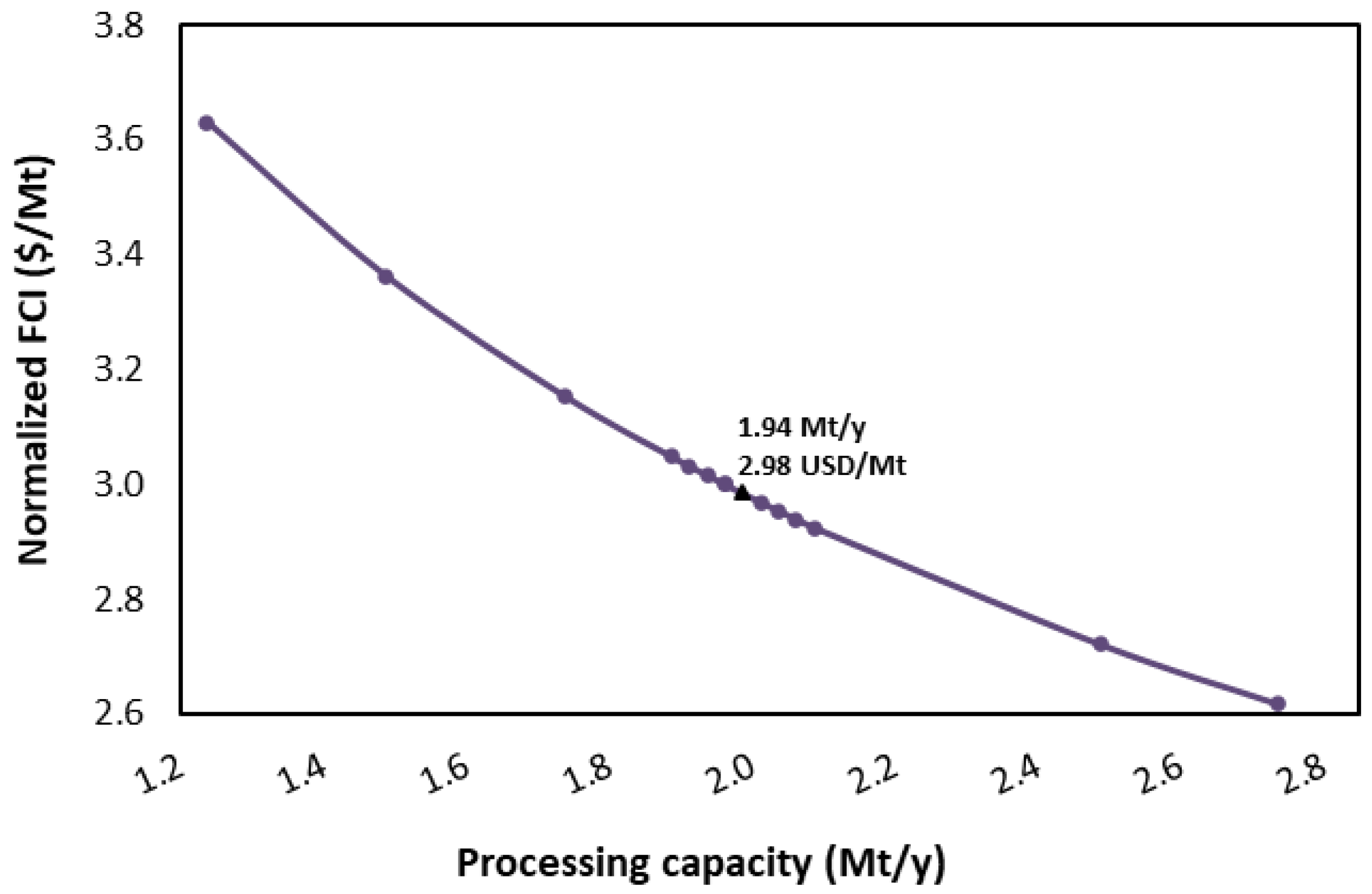
| Processing capacity (t/year) | 1,937,247.91 |
| Main product flow (t/year) | 933,777.85 |
| Raw material cost (USD/t) | 350.00 |
| Main product cost (USD/kg) | 1282.50 |
| Plant life (years) | 20 |
| Salvage value | 10% of depreciable FCI |
| Construction time | 3 years |
| Location | Latin America |
| Tax rate | 35% |
| Discount rate | 12.75% |
| Capacity operated | 50% the first year, 70% the second year, 100% from the third year onwards |
| Subsidies (USD/year) | 0 |
| Process type | Proven process |
| Process control | Digital |
| Type of project | Plant on unconstructed land |
| Type of soil | Soft clay |
| Contingency percentage (%) | 60 |
| Tank design code | ASME |
| Vessel diameter specification | Internal diameter |
| Operator hour cost (USD/h) | 30 |
| Supervisor hourly cost (USD/h) | 35 |
| Salaries per year | 13 |
| Utilities | Gas, water, steam, electricity |
| Process fluids | Liquid–gas |
| Depreciation method | Linear |
| Total Product Cost (TPC) | Total (USD/Year) |
|---|---|
| Raw materials | 821,863,576.21 |
| Utilities (U) | 971,422,578.00 |
| Maintenance and repairs (MR) | 4,580,753.53 |
| Operating supplies | 687,113.03 |
| Operating labor (OL) | 2,041,200.00 |
| Direct supervision and clerical labor | 306,180.00 |
| Laboratory charges | 204,120.00 |
| Patents and royalties | 916,150.71 |
| Direct production costs (DPCs) | 1,802,021,671.48 |
| Depreciation and amortization (DA) | 4,126,330.58 |
| Local taxes | 2,748,452.12 |
| Insurance | 916,150.71 |
| Interest/rent | 1,740,686.34 |
| Fixed charges (FCHs) | 9,531,619.75 |
| Plant overhead (POH) | 1,224,720.00 |
| Total manufacturing cost (TMC) | 1,812,778,011.23 |
| General expenses (GEs) | 453,194,502.81 |
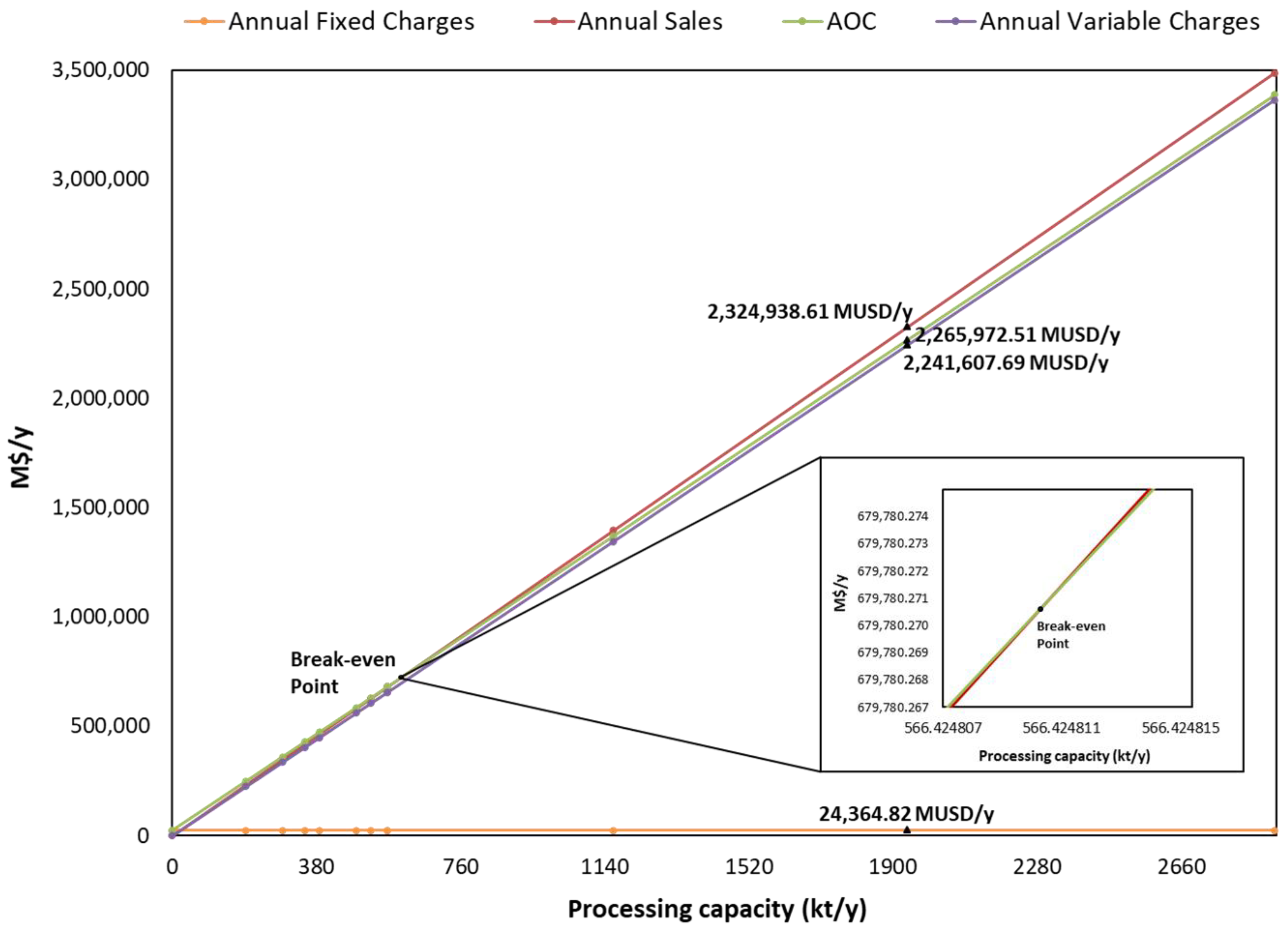
| Total product cost (TPC) | 2,265,972,514.03 |
| Capital Costs | Total |
|---|---|
| Cost of equipment (USD) | 15,218,349.15 |
| Delivered purchased equipment cost (USD) | 18,262,018.98 |
| Purchased equipment (installed; USD) | 5,478,605.69 |
| Instrumentation (installed; USD) | 2,191,442.28 |
| Piping (installed; USD) | 5,478,605.69 |
| Electrical network (installed; USD) | 3,469,783.61 |
| Buildings (including services; USD) | 9,131,009.49 |
| Services facilities (installed; USD) | 7,304,807.59 |
| Total DFCI (USD) | 51,316,273.33 |
| Land (USD) | 730,480.76 |
| Land improvements (USD) | 7,304,807.59 |
| Engineering and supervision (USD) | 9,496,249.87 |
| Equipment (R+D; USD) | 1,826,201.90 |
| Construction costs (USD) | 6,209,086.45 |
| Legal expenses (USD) | 182,620.19 |
| Contractors’ fees (USD) | 3,592,139.13 |
| Contingency (USD) | 10,957,211.39 |
| Total IFCI (USD) | 40,298,797.28 |
| Fixed capital investment (FCI; USD) | 91,615,070.61 |
| Working capital (WCI; USD) | 73,292,056.49 |
| Start-up (SUC; USD) | 9,161,507.06 |
| Total capital investment (TCI; USD) | 174,068,634.17 |
| Salvage value FCI (USD) | 9,088,458.99 |
| Annualized fixed costs (AFCs; USD/year) | 4,126,330.58 |
| Indicator | Total |
|---|---|
| Gross profit (depreciation not included) (GP; USD) | 58,966,096.31 |
| Gross profit (depreciation included) (DGP; USD) | 54,839,765.73 |
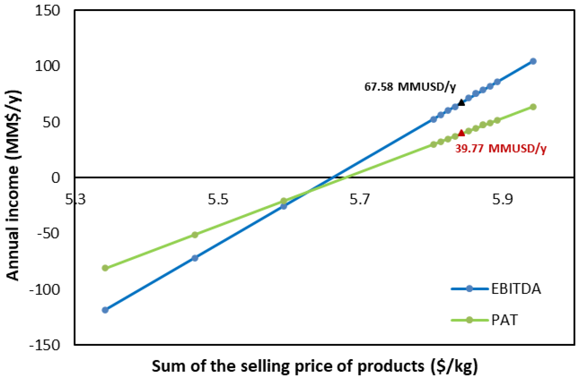
| Profitability after tax (PAT; USD) | 39,772,178.30 |
| Economic potentials 1 (EP1; USD/year) | 1,503,075,034.13 |
| Economic potentials 2 (EP2; USD/year) | 531,652,456.13 |
| Economic potentials 3 (EP3; USD/year) | 58,966,096.31 |
| Cumulative cash flow (CCF; 1/year) | 0.34 |
| Payback period (PBP; years) | 2.29 |
| Depreciable payback period (DPBP; years) | 4.14 |
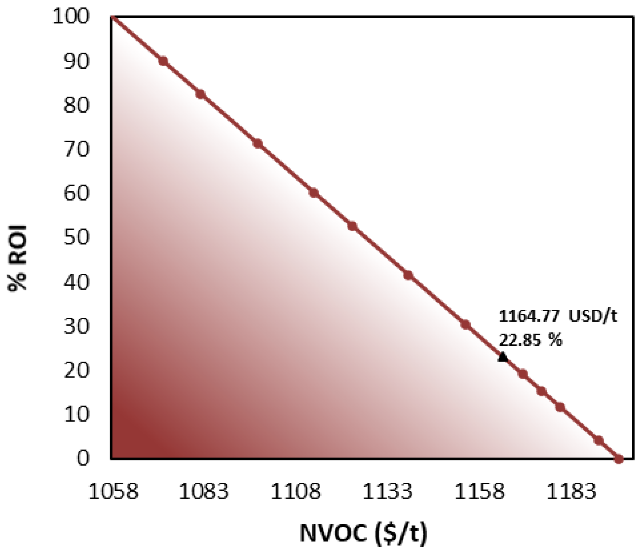
| Return on investment (% ROI) | 22.85 |
| Net present value (NPV; MMUSD) | 68.87 |
| Annual cost/revenue (ACR) | 9.66 |
| Internal rate of return (% IRR) | 29.34 |
| Normalized variable operating costs (NVOCs; USD/t-rm) | 1164.77 |
| Annualized total operating costs (AOCs; USD/year) | 2,265,972,514.03 |
| Indicator | Total |
|---|---|
| Earnings before taxes (EBT; USD) | 53,099,079.39 |
| Earnings before interest and taxes (EBIT; USD) | 54,839,765.73 |
| Earnings before interest, taxes, depreciation, and amortization (EBITDA; USD) | 67,581,565.35 |
Disclaimer/Publisher’s Note: The statements, opinions and data contained in all publications are solely those of the individual author(s) and contributor(s) and not of MDPI and/or the editor(s). MDPI and/or the editor(s) disclaim responsibility for any injury to people or property resulting from any ideas, methods, instructions or products referred to in the content. |
© 2025 by the authors. Licensee MDPI, Basel, Switzerland. This article is an open access article distributed under the terms and conditions of the Creative Commons Attribution (CC BY) license (https://creativecommons.org/licenses/by/4.0/).
Share and Cite
García-Maza, S.; González-Delgado, Á.D. Technical–Economic Assessment and FP2O Technical–Economic Resilience Analysis of the Gas Oil Hydrocracking Process at Large Scale. Sci 2025, 7, 17. https://doi.org/10.3390/sci7010017
García-Maza S, González-Delgado ÁD. Technical–Economic Assessment and FP2O Technical–Economic Resilience Analysis of the Gas Oil Hydrocracking Process at Large Scale. Sci. 2025; 7(1):17. https://doi.org/10.3390/sci7010017
Chicago/Turabian StyleGarcía-Maza, Sofía, and Ángel Darío González-Delgado. 2025. "Technical–Economic Assessment and FP2O Technical–Economic Resilience Analysis of the Gas Oil Hydrocracking Process at Large Scale" Sci 7, no. 1: 17. https://doi.org/10.3390/sci7010017
APA StyleGarcía-Maza, S., & González-Delgado, Á. D. (2025). Technical–Economic Assessment and FP2O Technical–Economic Resilience Analysis of the Gas Oil Hydrocracking Process at Large Scale. Sci, 7(1), 17. https://doi.org/10.3390/sci7010017