Article

From Radar Sensor to Floating Car Data: Evaluating Speed Distribution Heterogeneity on Rural Road Segments Using Non-Parametric Similarity Measures

1
Department of Civil, Constructional and Environmental Engineering, University of Rome La Sapienza, Via Eudossiana 18, 00184 Rome, Italy
2
Department of Civil, Environmental and Mechanical Engineering, University of Trento, Via Mesiano 77, 38123 Trento, Italy
3
Faculty of Technological & Innovation Sciences, Universitas Mercatorum, Piazza Mattei, 10, 00186 Rome, Italy
*
Author to whom correspondence should be addressed.
Submission received: 17 July 2024 / Revised: 10 August 2024 / Accepted: 22 August 2024 / Published: 2 September 2024
(This article belongs to the Section Computer Sciences, Mathematics and AI)

Abstract

:
Rural roads, often characterized by winding paths and nearby settlements, feature frequent curvature changes, junctions, and closely spaced private accesses that lead to significant speed variations. These variations are typically represented by average speed or v85 profiles. This paper examines complete speed distributions along rural two-lane roads using Floating Car Data (FCD). The Wasserstein distance, a non-parametric similarity measure, is employed to compare speed distributions recorded by a radar Control Unit (CU) and a selected FCD sample. Initially, FCD speeds were validated against CU speeds. Subsequently, differences in speed distributions between the CU location and specific sections identified by sharp curves, intersections, or accesses have been assessed. The Wasserstein Distance is proposed as the most effective synthetic indicator of speed distribution variability along roadways, attributed to its metric properties. This measure offers a more concise and immediate assessment compared to an extensive array of statistical metrics, such as mean, median, mode, variance, percentiles, v85, interquartile range, kurtosis, and symmetry, as well as qualitative assessments derived from box plot trends.

1. Introduction

Monitoring and analyzing vehicle speed distribution is crucial for understanding traffic flow dynamics and ensuring road safety, particularly in rural road segments [1]. Traditional methodologies predominantly utilize fixed sensors deployed at predetermined locations to record instantaneous vehicle speeds. This approach facilitates the generation of empirical speed distributions and enables the computation of related statistical measures, thereby offering a discrete snapshot of speed patterns at specific points along the roadway. However, these fixed-point measurements inherently lack continuity, as they can only offer intermittent data points based on the placement and density of sensors [2]. Fixed sensors, while useful, present a limitation in that they often fail to correlate data from individual vehicles across multiple sections. As a result, traffic behavior between points must be inferred through aggregate data comparisons or interpolations, leaving significant gaps in the understanding of speed distribution along the entire road segment [3]. For instance, methods such as linear, polynomial, or spline interpolations are commonly employed to estimate speed trends between sensor points, but these techniques do not capture the true variability and heterogeneity of speed distributions over continuous distances [4].
The advent of Floating Car Data (FCD) technology has introduced a transformative approach to traffic analysis by providing near-continuous temporal tracking of equipped vehicles. Li et al. [5] presented a computationally simple and robust cross-validation method for reconciling traffic speed measurements from probe and stationary sensors, effectively identifying discrepancies using both simulation models and real-world freeway data. Although FCD samples represent a smaller fraction of the total vehicle population, they offer a high level of detail in spatial and temporal segmentation, enhancing traffic data accuracy [6]. To optimize this accuracy, Altintasi et al. [7] propose a method to assess the traffic Penetration Rate (PR) of commercial FCD by comparing its speed estimation to Ground Truth (GT) data, finding that a PR of 15% significantly improves FCD quality, with a suggested PR of around 5% for commercial FCD. Despite the increasing volume of research utilizing FCD for assessing mean speeds, percentiles, and other statistics along road segments, there is a noticeable gap in the literature regarding the analysis of complete speed distributions. For instance, Budimir et al. [8] explore the use of mobile vehicles to collect real-time traffic flow data through FCD and Probe vehicles, highlighting their efficiency, cost-effectiveness, and extensive coverage for achieving sustainable mobility, supported by technologies like GIS, GNSS, and wireless communication. Ambros et al. [9] investigate the use of FCD for proactively identifying risk locations on rural roads by analyzing GPS-derived speeds and their relationship with accident frequency, highlighting practical feasibility and implications for rural safety monitoring and evaluation. Fabrizi and Ragona [10] present a model for short-term traffic speed forecasting using an FCD system, which enhances coverage without expensive infrastructure and provides real-time traffic speed information across a road network. Zhang et al. [11] developed a method for identifying bottlenecks using FCD, employing speed difference as a primary indicator and speed-at-capacity as a secondary indicator to evaluate bottlenecks by duration, affected distance, delay, and cause.
This paper aims to address this gap by proposing a novel method for evaluating variations in vehicle speed distribution along rural road segments with various geometric and functional characteristics. We utilize a validated FCD sample cross-referenced with data from a fixed control station to apply a non-parametric similarity measure—specifically, the 1-Wasserstein distance—to compare speed histograms at closely spaced intervals along the road. By highlighting areas of homogeneity and heterogeneity in speed distributions, this approach allows for a detailed examination of how physical and geometric features of the road, such as curvature, lane count, intersections, and access points, influence driving behavior. The continuous nature of FCD data, combined with sophisticated similarity measures, enables a more comprehensive understanding of speed distribution heterogeneity. This, in turn, can inform more effective traffic management strategies and road design improvements aimed at enhancing safety and efficiency on rural roads.

2. Materials

The evaluation of operating speed is pivotal in assessing the effects of roadside and geometric features on both collision occurrence and severity. Indeed, roadside features increase collision frequency while reducing speed, whereas geometric features have the opposite effect, and lower operating speeds lead to a reduction in collision frequency [12]. The 85th percentile speed, commonly referred to as the operating speed, is typically used to characterize the distribution of vehicle speeds. This percentile provides an estimate of the speed below which 85% of the traffic is traveling, offering a more robust representation of typical driving behavior than mean speed. Historically, operating speed models have relied on data from inductive loops and magnetic sensors, which capture vehicle speeds at specific locations [13]. These sensors provide detailed temporal data but are limited in their spatial coverage, as they only record speeds at their installation sites. Recent advancements have introduced Floating Car Data (FCD), derived from vehicles equipped with GPS devices. FCD offers comprehensive spatiotemporal insights by tracking vehicle movements across entire road networks, thus enabling more accurate modeling of operational speeds.
Floating Car Data (FCD) refers to speed and location data collected from vehicles that are part of the traffic stream and equipped with GPS tracking systems. These data are valuable because they provide continuous monitoring of vehicle speeds over extended areas, capturing real-world driving behavior across different road segments. FCD is advantageous due to its ability to collect data over both temporal and spatial domains, giving a holistic view of traffic dynamics over a network rather than at discrete points [2]. However, one challenge associated with FCD is ensuring the representativeness of the data, given that it is often collected from a limited subset of the total vehicle population [7].
In contrast, fixed sensors (such as radar units, inductive loops, and ANPR cameras) are deployed at specific locations along the roadway to capture the instantaneous speeds of passing vehicles. These sensors provide high-resolution temporal data for vehicle speeds at particular points, offering insights into traffic flow characteristics at fixed locations. However, the major limitation of fixed sensors is their spatial restriction; they cannot provide continuous data along the road network and are unable to capture speed variations beyond their immediate vicinity [4].
In this research, we have used data from the Automatic Statistical Traffic Detection System managed by ANAS SpA, which operates within the Italian national road network. This system uses a variety of sensors to collect traffic data, which is centralized in the Platform for Monitoring and Analysis (PANAMA). The accuracy and reliability of this data are ensured through rigorous validation procedures. The fixed-point data were collected over three distinct months—August 2018, February 2019, and May 2019—within the Veneto Region. The data included the following variables:
  • Time Reference: Date and time of data acquisition;
  • Lane: The specific lane on which the vehicle was traveling;
  • Direction: The direction of travel;
  • Speed: The speed of the vehicle recorded in km/h;
  • Vehicle Class: A code identifying the vehicle type (e.g., cars and trucks).
The FCD was obtained from a commercial provider that aggregates GPS data from over four million vehicles equipped with black boxes and from approximately 1.5 million smartphone applications. The dataset contained nearly one billion data points for the same time periods and region as the fixed sensor data. Key variables included the following:
  • Identification Code: Unique identifier for each data point;
  • Longitude and Latitude: Vehicle location coordinates in WGS 84 format;
  • Direction: Direction of travel expressed as an azimuth angle;
  • Speed: Vehicle speed at the time of signal emission;
  • Date and Time: Timestamp of the GPS signal;
  • Signal Quality: Quality of the GPS signal;
  • Vehicle ID: Unique identifier for each vehicle;
  • Vehicle Type: Classification of the vehicle.
Both data sources provided extensive datasets that allowed for a comprehensive analysis of vehicle speed profiles across different road segments.

3. Methods

This study explores the assessment of statistical homogeneity and heterogeneity in traffic data, emphasizing the importance of understanding these concepts for evaluating the consistency of traffic flow patterns. The analysis employs both parametric and non-parametric tests to compare data distributions, particularly focusing on how variations in traffic flow can be interpreted through measures of similarity and dissimilarity. Histograms and series of histograms are utilized to represent the distribution of large datasets, capturing both spatial and temporal variations in traffic collected from fixed sensors and FCD. Advanced similarity measures, such as the Wasserstein distance with the L1 norm, are applied to quantify the differences between data distributions, offering a comprehensive approach to understanding traffic dynamics. This approach helps to identify consistent patterns or anomalies in traffic behavior, thereby providing insights into the macroscopic and microscopic variations influenced by changing road conditions and user behaviors. The study highlights the necessity of employing robust statistical techniques to manage and analyze large datasets, ensuring a detailed evaluation of traffic flow characteristics across different segments and periods.

3.1. Homogeneity and Non-Homogeneity

In statistical analysis, the terms “homogeneity” and “heterogeneity” are crucial for understanding and interpreting data characteristics, where homogeneity denotes uniformity and similarity across datasets, and heterogeneity signifies variability and diversity within or between datasets. These concepts are essential for assessing consistent statistical properties across different segments or among multiple datasets, particularly in relation to probability distributions of random variables [14]. Heterogeneity and homogeneity can be defined by various parameters such as mean, variance, skewness, and kurtosis, which are key considerations when comparing multiple samples to understand differences or similarities between groups, whether originating from the same or different populations [15].
Traditional statistical methods include both parametric and non-parametric tests for evaluating and comparing samples. Parametric tests are suitable when assumptions about data distributions, such as normality, are met, while non-parametric tests are used when data do not conform to specific distributional criteria [16]. The concepts of spatial and temporal homogeneity and heterogeneity are vital in time series analysis, where a time series is homogeneous if its statistical properties, like mean and variance, remain constant over time [17]. This homogeneity simplifies analysis and forecasting using models such as ARIMA. Conversely, heterogeneous time series, with non-constant statistical properties, require more advanced techniques like ARCH for analyzing volatility clustering [18].
In traffic analysis, homogeneity and heterogeneity can describe the spatial distribution of vehicles along a road segment, as well as vehicle types and driving behaviors [19]. Homogeneous conditions imply uniformity and predictability, simplifying traffic modeling, while heterogeneity reflects real-world traffic variability influenced by factors such as traffic composition, driving behaviors, road design, and external conditions [20]. The gradient between homogeneity and heterogeneity underscores the need for measures that can quantify the extent of similarity or dissimilarity in various contexts [21].
Similarity and dissimilarity measures are prominent tools for comparing datasets, providing a refined approach to assess the degree of resemblance or divergence between them [22]. These measures are particularly important in machine learning and data mining, where they help quantify relationships, identify patterns, and classify clusters within large datasets, thereby addressing the complexities of modern data analysis challenges [21]. The application of these measures in data science facilitates effective analysis and interpretation of large datasets, essential for pattern recognition and clustering [22].

3.2. Histograms and Histograms Series

Data science is characterized by its focus on large and complex datasets and the use of advanced computational techniques to create predictive models and algorithms that can process and analyze these data efficiently [16]. Although statistical principles provide the foundational theories and techniques for data science, the field extends beyond these basics by integrating extensive dataset management, real-time data processing, and the application of complex algorithms. These methodologies delve into pattern recognition, machine learning, and big data technologies, expanding the scope of traditional statistical analysis [17,18].
Large-scale datasets, often continuously expanding due to high-frequency data collection from sensor networks, are now prevalent. These sensors capture data that are dependent on both time and geographic positioning, making the assessment of temporal and spatial correlations particularly valuable for practical applications [23]. In the context of road infrastructures, the proliferation of various sensor types has dramatically increased the volume of data available for analyzing driving behavior and traffic conditions in real-world scenarios. Floating Car Data (FCD) exemplifies this trend by providing extensive data on vehicle speed and other parameters, which are linked to time and geographic coordinates. These data can be aligned to a single temporal or positional variable, facilitating detailed analysis at specific points along a road axis.
When measuring variables like vehicle speed over time or location, especially when the interest lies in group behavior rather than individual specifics, it is beneficial to represent the data through a series of distributions rather than aggregated metrics. This approach allows for a more informative representation. The choice of representation can be parametric, such as a Gaussian mixture model, or nonparametric, like a histogram or kernel-based density estimator [24]. Histograms are widely used in this context due to their balance between simplicity and accuracy. They serve as effective nonparametric density estimators for data analysis and visualization, enabling the derivation of summary metrics like entropy, which captures the underlying data density [25].
The study of data through histograms has led to a new paradigm in statistical analysis known as symbolic data analysis [26]. Histograms offer a practical method for standardizing and condensing the statistical characteristics of data, especially when dealing with large and complex datasets. While this method may lose some distributional nuances depending on bin count, it is advantageous due to its assumption-free nature and computational efficiency. Continuous research into binning strategies and innovative methodologies is enhancing their utility in statistical and machine learning frameworks [17,27,28].
The concept of histograms, initially introduced by Pearson, involves dividing a continuous variable X into a set of contiguous I ϕ intervals (bins) with associated π ϕ weights, providing a straightforward model for representing empirical distributions [29]. A histogram P is thus represented by a set of Φ ordered pairs ( I ϕ , π ϕ ), where π ϕ is a non-negative measure of a probability distribution on the domain of X such that [25]
ϕ = 1 Φ π ϕ = 1           w i t h   π ϕ 0 I ϕ I ϕ = ,   ϕ   ϕ                     ϕ = 1 Φ I ϕ = X m i n ,   X m a x ,                    
The time complexity of computing a univariate histogram with a fixed bin width depends on the number of bins Φ in the histogram and the number of data points n being processed, where Φ is usually much smaller than n . Thus, a fixed bin width histogram is completely classified by two parameters, the bin width and the bin origin, and expressed as a set of pairs P = I ϕ , π ( P ) ϕ . The computation of histograms, especially those with fixed bin widths, is influenced by the number of bins and data points processed, making them computationally efficient for large datasets [26]. While various methods exist to determine the optimal value for Φ , such as Scott’s normal rule, Freedman-Diaconis rule, and Mosteller-Tukey rule [30,31,32], these methods often assume specific distribution shapes and may not universally apply. Varying the bin width can help balance noise reduction and representation precision, making histograms a flexible tool for data analysis.
Density estimators like kernel methods and Gaussian mixture models offer smoother representations of underlying distributions compared to histograms. However, in cases where extreme smoothness is not necessary, histograms significantly reduce computational complexity. This efficiency extends to a series of histograms used to represent sequences of distributions, providing a valuable tool for analyzing ordered sequences in both temporal and spatial dimensions [33,34]. In symbolic data analysis, histogram series represent a sequence of observations where each realization is characterized by a histogram variable, facilitating the analysis of complex data structures [34].

3.3. Similarity and Dissimilarity Measures in Large Datasets and Histogram Series

As previously discussed, comparing distributions (e.g., among distributions in a series) is a significant area in pattern classification, data clustering, image processing, and computer vision, where finding histogram similarity is a recurrent technique [21,22]. Histogram similarity evaluations are also crucial in time series analysis. By dividing time series into sequential sub-series, histograms can present the frequency of values for these sub-series, enabling the study of probability distribution variations using similarity analysis [35]. This approach has been used to study fine correlations in physical, chemical, biochemical, or hydrological systems measurements [36,37,38,39] and to define clusters for time series in various fields [40].
Similarity or dissimilarity comparisons of statistical properties among samples through histogram analysis can be divided into bin-by-bin and cross-bin methods [41,42]. Bin-by-bin methods compare corresponding bins between histograms without considering correlations between neighboring bins. For instance, comparing histograms P = I ϕ , π ( P ) ϕ and Q = I ϕ , π ( Q ) ϕ , these techniques measure the difference between corresponding bins only. Despite being straightforward and computationally efficient for large datasets, bin-by-bin methods are sensitive to bin size and slight translations of weights can significantly affect similarity evaluation. Examples include histogram intersection, histogram correlation, total variation distance, χ2 statistic, and Bhattacharyya distance [43].
In contrast, cross-bin methods compare both corresponding and non-corresponding bins among histograms, considering correlations between neighboring bins to provide a more comprehensive comparison [41]. These methods are less sensitive to bin size and can represent similarities and dissimilarities more effectively.
Using these methods, a measure of similarity or dissimilarity can be defined, conceptually resembling a form of “distance”. The decision regarding histogram similarity generally depends on the specific distance measure employed. Histograms are considered similar if the “distance” between them is below a certain threshold. Alternatively, a similarity metric increasing with resemblance can be used, where similarity exceeds a threshold [44].
These similarity measures can be defined as divergences or metrics, the latter also known as distances in the mathematical sense. In general, a measure D is a mapping p , q R + with the following properties:
  • D(p,q) ≥ 0 for all p and q defined over R (non-negativity);
  • D(p,q) = 0 if and only if p = q (identity of indiscernible).
A metric, or distance, is a divergence with
  • D(p,q) = D(q,p) (symmetry);
  • D(p,q) ≤ D(p,g) + D(g,q) for any distribution g over R (triangle inequality).
Depending on which properties are fulfilled, measures can be classified differently. We refer to it as a distance when the measure satisfies all the aforementioned properties. Pseudo-distances do not satisfy the identity of indiscernible, quasi-distances do not fulfill symmetry, semi-distances do not fulfill triangle inequality, and divergences do not comply with symmetry and triangle inequality [45].
In this paper, the 1-Wasserstein (1W) distance, also known as the Kantorovich–Wasserstein (KW) metric or Earth Mover’s Distance (EMD), will be introduced and discussed for practical use in vehicle speed distribution analysis. The 1W distance is a similarity metric following a cross-bin approach defined using the Optimal Transport Problem (OTP) in the Kantorovich formulation.
The genesis and definitions of this similarity measure in the literature will be reviewed, along with its important properties. Algorithms for comparing pairs of histograms with an equal number of bins and the same origin, specifically from speed samples of vehicular speeds at different points along a road axis, will be proposed. Criteria for identifying a comprehensive similarity measure of speed distribution variability for quasi-continuous analysis of a road segment will be discussed based on the specific properties of this measure.

3.4. Wasserstein Metric

The p -Wasserstein ( p W) distance D p W , also known as the Wasserstein metric, Kantorovich metric, or Earth Mover’s Distance (EMD) when p = 1, was first defined by Leonid Kantorovich in the context of optimal transport planning for goods and materials [46]. The term “Vasershtein distance” was later coined by Dobrushin, following Vaseršteĭn’s work [47,48].
The concept is rooted in the problem of “transporting” one mass distribution to another one while minimizing the transport cost, a problem originally introduced by Gaspard Monge in 1781 [49]. Kantorovich extended this into a formal mathematical framework, leading to the Monge–Kantorovich transportation problem [46]. Optimal transport (OT) involves finding a cost-effective way to map a source distribution to a target distribution while minimizing transport costs. This is illustrated in Figure 1, which shows Monge’s OT formulation. The OT problem assumes mass conservation and non-negativity, meaning both the source and target must have equal non-negative mass. These principles naturally align with the framework of probability densities [46]. Given a cost function c : X × Y 0 , , Monge’s problem seeks a transport map T * : X Y that minimizes the total transport cost
c T = X c x , T x · p x d x
Kantorovich’s formulation generalizes this by seeking a probability measure ν that minimizes cost over all possible transport plans, as follows:
i n f X × Y c x , y d ν x , y | ν   ϵ   Γ p , q
Here, Γ p , q represents all probability measures with marginals p and q . The p -Wasserstein distance D p W is then defined using the cost function, where the value of p determines the severity of penalties for mass transport. For one-dimensional distributions, the p -Wasserstein distance is given by
D p W p , q = 0 1 F p 1 s F q 1 s p d s 1 p
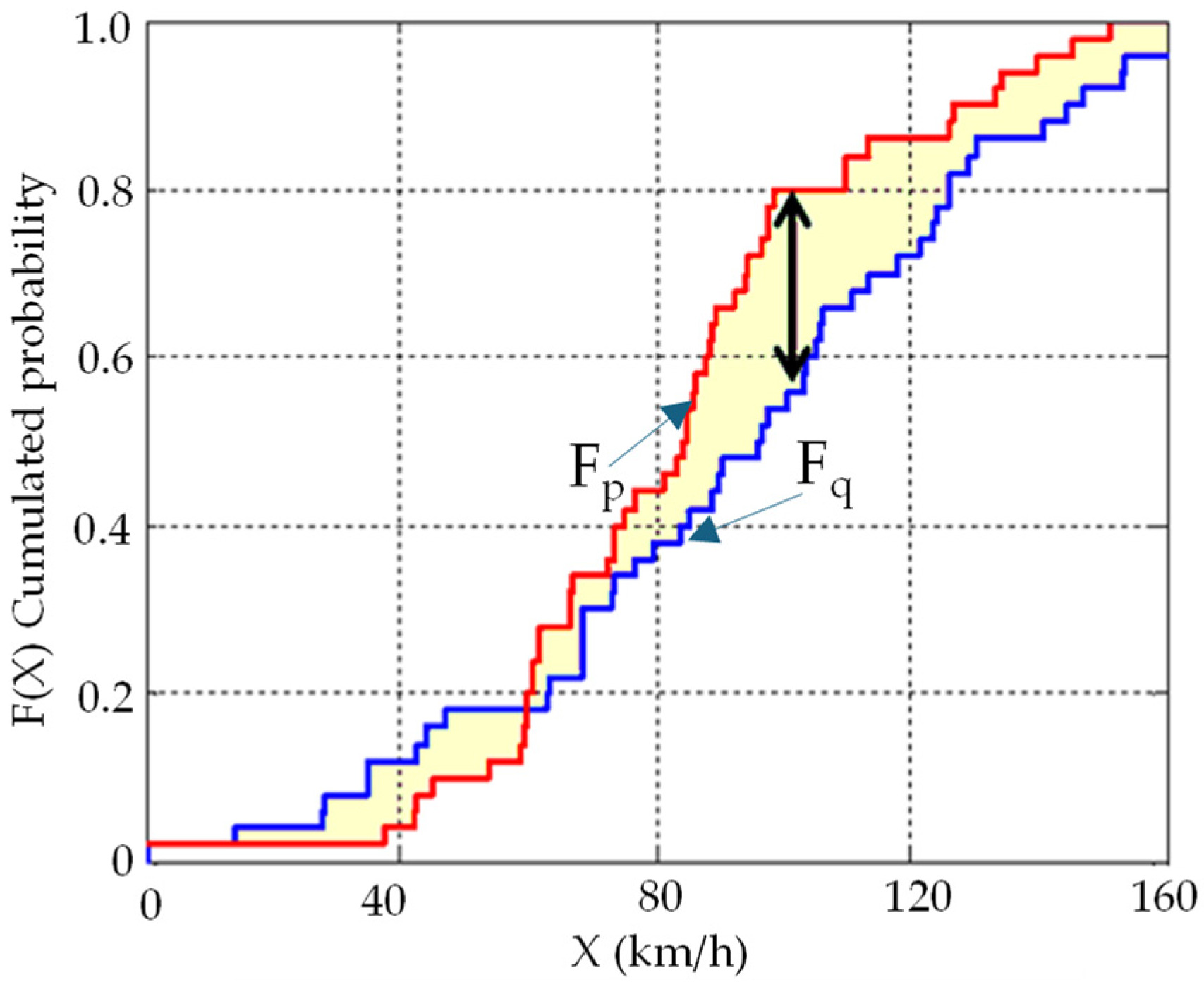
In the special case where p = 1 , the 1-Wasserstein distance measures the total area between two CDFs F p and F q , providing a comprehensive measure of distributional similarity [50,51]. This is particularly useful for comparing empirical distributions, such as vehicle speed distributions along a road, where data are often represented as step functions or histograms [52]. The 1-Wasserstein distance effectively captures differences across these distributions, including both horizontal and vertical discrepancies, as illustrated in Figure 2.
For histogram comparisons, D 1 W can be efficiently computed by summing the differences between corresponding bins, as follows:
E M D ϕ = 1 = 0 E M D ϕ + 1 = π ( P ) ϕ + E M D ϕ π ( Q ) ϕ w i t h   ϕ = 1 , Φ D 1 W P , Q = ϕ = 1 Φ E M D ϕ
The 1-Wasserstein distance is a robust metric for comparing distributions, making it valuable in applications ranging from computer vision to traffic analysis. It allows for a comprehensive similarity measure that is more informative than traditional metrics like the Kolmogorov–Smirnov distance, which only captures maximum vertical differences between distributions [53,54], as illustrated in Figure 2.
For discrete one-dimensional histograms, it can be rigorously demonstrated that the D 1 W P , Q is bounded above by ( Φ 1 ). This scenario occurs when the experimental distribution p is entirely concentrated in the first bin ( ϕ = 1 ) of P , w h i l e   t h e   e x p e r i m e n t a l   d i s t r i b u t i o n   q is entirely concentrated in the last bin ( ϕ = Φ ) of Q or vice versa. This upper bound D 1 W P , Q facilitates its normalization, yielding D 1 W ~ P , Q ranging from 0, indicating complete overlap of the histograms (total similarity), to 1, representing the maximum dissimilarity between them.

4. Speed Probability Distribution on Two-Lane Road Segments

Although the assumption of homogeneous conditions simplifies classic traffic flow theory and modeling, real-world traffic flow exhibits significant heterogeneity. Similarity measures effectively evaluate the gradient of similarity between homogeneous and heterogeneous conditions, ranging from maximal to minimal similarity. In traffic analysis, studying how traffic flow characteristics vary along a road segment is crucial, particularly in understanding vehicular speed trends on highways. This knowledge is vital for highway design, performance and safety verification, and regulatory compliance monitoring.
Analyzing vehicle speed data along a highway segment provides insights into the probability distribution of speeds at different sections. By examining a sequence of sections, the speed behaviors form a sequence of random variables. Instantaneous speed samples from vehicles allow the inference of probability distributions, beyond simple sample statistics like centrality, dispersion, and percentiles, including v85 profiles.
This paper section illustrates how the 1-Wasserstein distance can represent variations in speed distribution along a highway segment. Using a limited sample of speeds from Floating Vehicles (FV) or Floating Car Data (FCD), validated by a larger sample from fixed monitoring devices, we can concisely capture these variations.

4.1. Establishing Baseline Data for Analyzing Speed Distribution Similarity

This study focuses on a secondary rural road that runs from Mestre (Venice) to Pesek (San Dorligo della Valle) in the province of Trieste. The section examined crosses the Veneto Region and is classified as a secondary rural road according to Italian standards (DM2001). It is characterized by variable geometric and functional features, such as curvature, access points, intersections, and lane numbers. The analysis centers on two specific segments of SS14: Segment 218, which extends from kilometer marker 12,000 to 22,000 in the descending direction (DESC), and Segment 3191, which extends from kilometer marker 4000 to 14,000 in the ascending direction (ASC). Segment km 4000–8000 features a dual carriageway with two lanes in each direction, with a total width of approximately 15 m. The presence of at-grade intersections that handle significant traffic volumes necessitates the inclusion of specialized lanes, such as left-turn lanes. Segment km 8000–13,470 has a single carriageway with one lane per direction, each lane being 3.5 m wide, and 1 m-wide shoulders on both sides. Segment km 12,000 to 22,000 also has a single carriageway with one lane per direction. However, at kilometer 17 + 750, the presence of an at-grade intersection with acceleration and deceleration lanes facilitates smoother turning maneuvers. Both segments—218 and 3191—are equipped with fixed monitoring stations that provide continuous data collection. For Segment 218, the fixed station is located at kilometer marker 17,085, while for Segment 3191, it is positioned at kilometer marker 9047. Data were collected from these stations during three distinct periods: August 2018, February 2019, and May 2019. The data collection for each of the three periods spanned the entire month. During these months, data were collected continuously without any intentional breaks in the collection process. These time frames were chosen to capture a representative sample of traffic conditions over different seasons.
The Floating Car Data (FCD) database, which contains detailed information on vehicle positions and speeds, was meticulously processed using map-matching techniques. These techniques align the recorded vehicle positions with the road segment’s progression, ensuring spatial accuracy. Additionally, vehicles that did not pass the fixed monitoring stations, or those lacking continuous trajectory and sufficient signal emission frequency (i.e., 1 Hz), were filtered out to maintain data integrity. To determine the lack of a continuous trajectory for a vehicle, specific criteria based on the consistency and completeness of the recorded GPS data have been applied:
  • Signal Frequency Check: Vehicles with data points recorded at frequencies lower than 1 Hz could indicate gaps in the trajectory and were flagged for further inspection;
  • Temporal and Spatial Continuity: For each vehicle, the sequence of recorded positions (latitude, longitude, and corresponding timestamps) has been examined to ensure that the vehicles followed a logical and continuous progression along the road. Significant gaps in time between successive data points, or abrupt, unrealistic jumps in spatial position (which could not be explained by the vehicle’s speed or the road’s geometry), were used as indicators of a non-continuous trajectory;
  • Cross-Reference with Road Geometry: If the trajectory data suggested that a vehicle deviated significantly from the expected path without any corresponding road features that could explain such a deviation (e.g., intersections, exits), this was considered a lack of continuity.
By establishing this comprehensive baseline data, including detailed descriptions of the road segments, fixed monitoring stations, and the processed FCD, the study provides a solid foundation for analyzing speed distribution similarity along the highway segments. This robust dataset enables a precise and accurate evaluation of traffic patterns and their variability, facilitating a deeper understanding of speed distributions under varying road and traffic conditions.

4.2. Speed Distributions Heterogeneity and Similarity Measure

The distance progression measurements for each Floating Vehicle (FV) and their corresponding instantaneous speeds were extracted from the entire database. These measurements, sampled at irregular intervals due to variable signal emission frequencies and vehicle speeds, resulted in non-uniform data points along the road track. To achieve a seamless speed representation across the monitored road segment, a cubic smoothing spline was applied to each vehicle’s distance progression and speed vectors. During the method selection phase, we considered alternatives like kernel smoothing and moving average. However, these were discarded in favor of the cubic smoothing spline. Kernel smoothing showed excessive variability with different bandwidths, and moving averages did not reliably capture local variations. Additionally, cubic smoothing spline is a robust method widely used for FCD in the literature [55], offering easily implementable solutions with a good balance between data flexibility and curve smoothness control. This third-degree polynomial function is implemented using Matlab R2020a’s ‘csaps’ function with a smoothing parameter of 2 × 10⁻⁴. After conducting preliminary analyses and cross-validations, this value provided a good compromise, capturing the data’s underlying trend while filtering out high-frequency noise. We tested various smoothing parameters and evaluated the fit quality and smoothness of the resulting curves.
Resampling of speeds was performed in virtual counting sections (VSs) along the highway segment, identified at uniform 10-m intervals from the initial point of the monitored stretch. The choice of a 10-m interval for the VSs along the highway segment was chosen as the optimal compromise, balancing detailed representation of road variations and efficient data use. It was based on several factors, considering that we aimed for granularity that allows effective analysis and accurate correlation of speed data with road characteristics. Preliminary analyses showed that a 10-m interval captures significant changes in road geometry, such as curvature, better than coarser intervals. Finer intervals would have led to over-detailing without significant advantages.
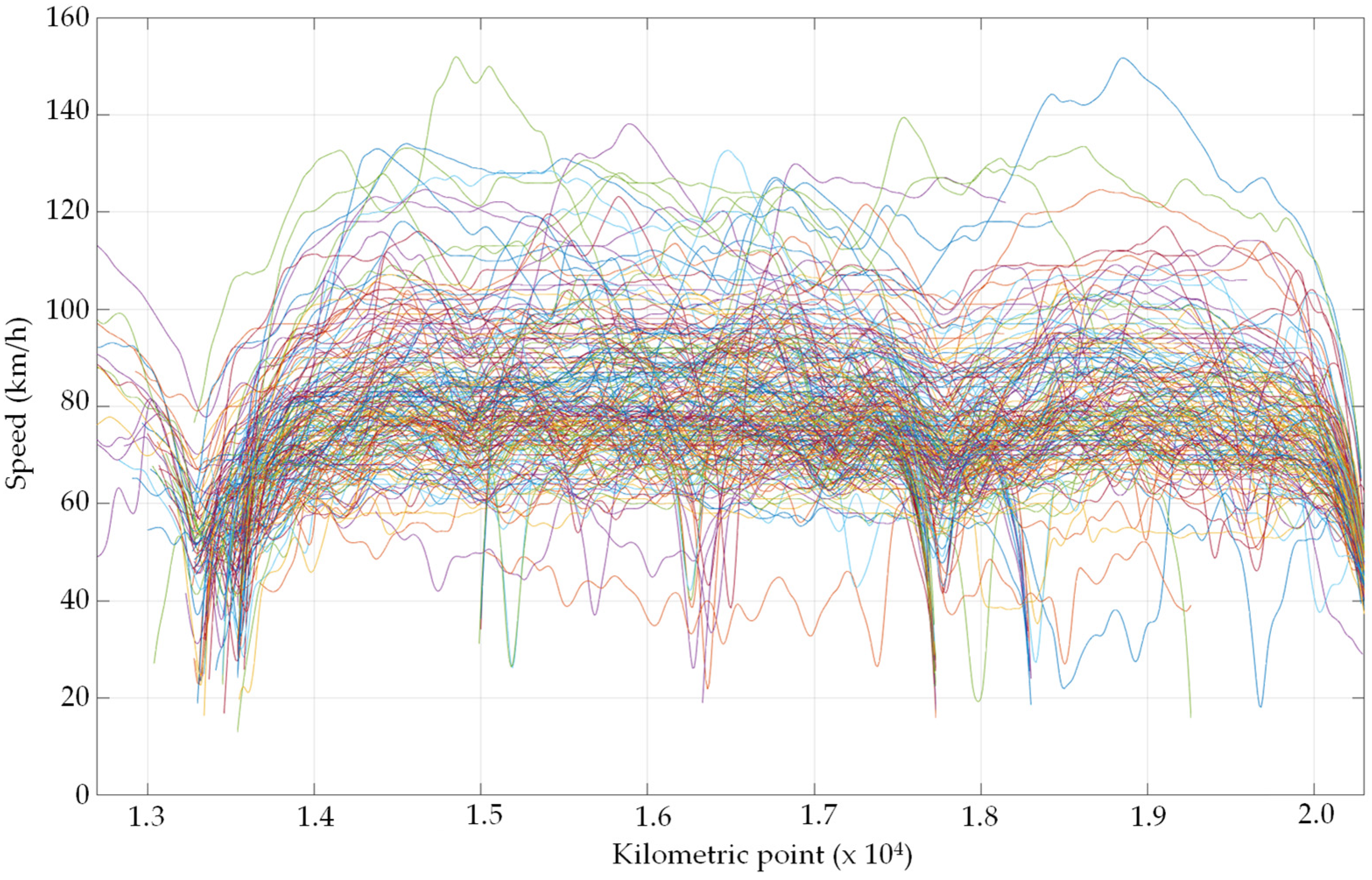
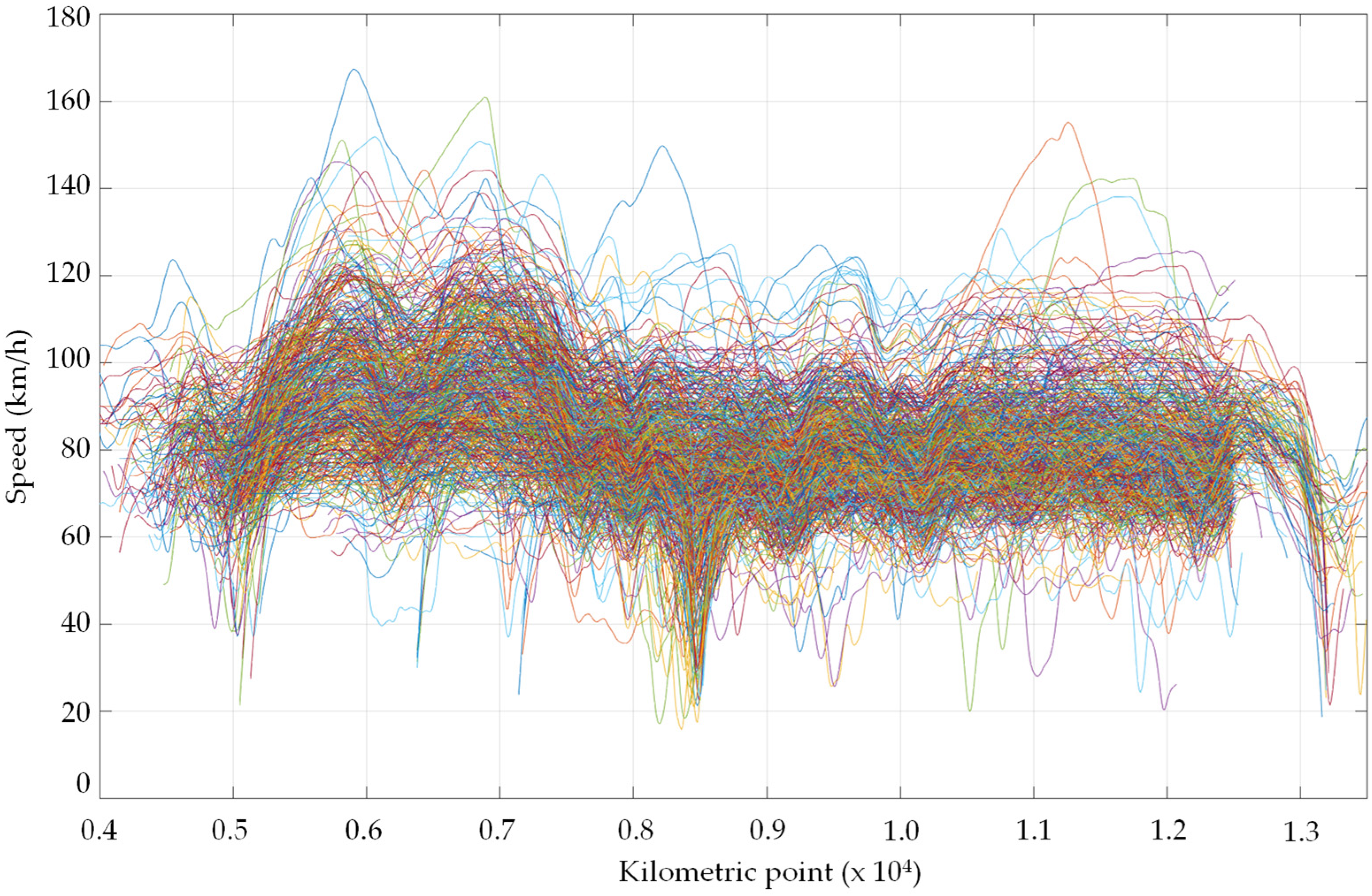
During our preliminary analysis, we observed that virtual tail sections with fewer than 10 vehicles resulted in excessively high variability in the data due to the small sample size. Thus, virtual tail sections collecting fewer than 10 speed values were excluded to minimize the influence of outliers and anomalies, ensuring that the data from each virtual section is representative of the behavior of a larger group. Figure 3 and Figure 4 display the smoothing splines for VSs with a minimum of 10 FVs in two segments of SS14: segment 218 (km 12,660 to km 20,310, DESC direction) and segment 3191 (km 4000 to km 13,470, ASC direction).
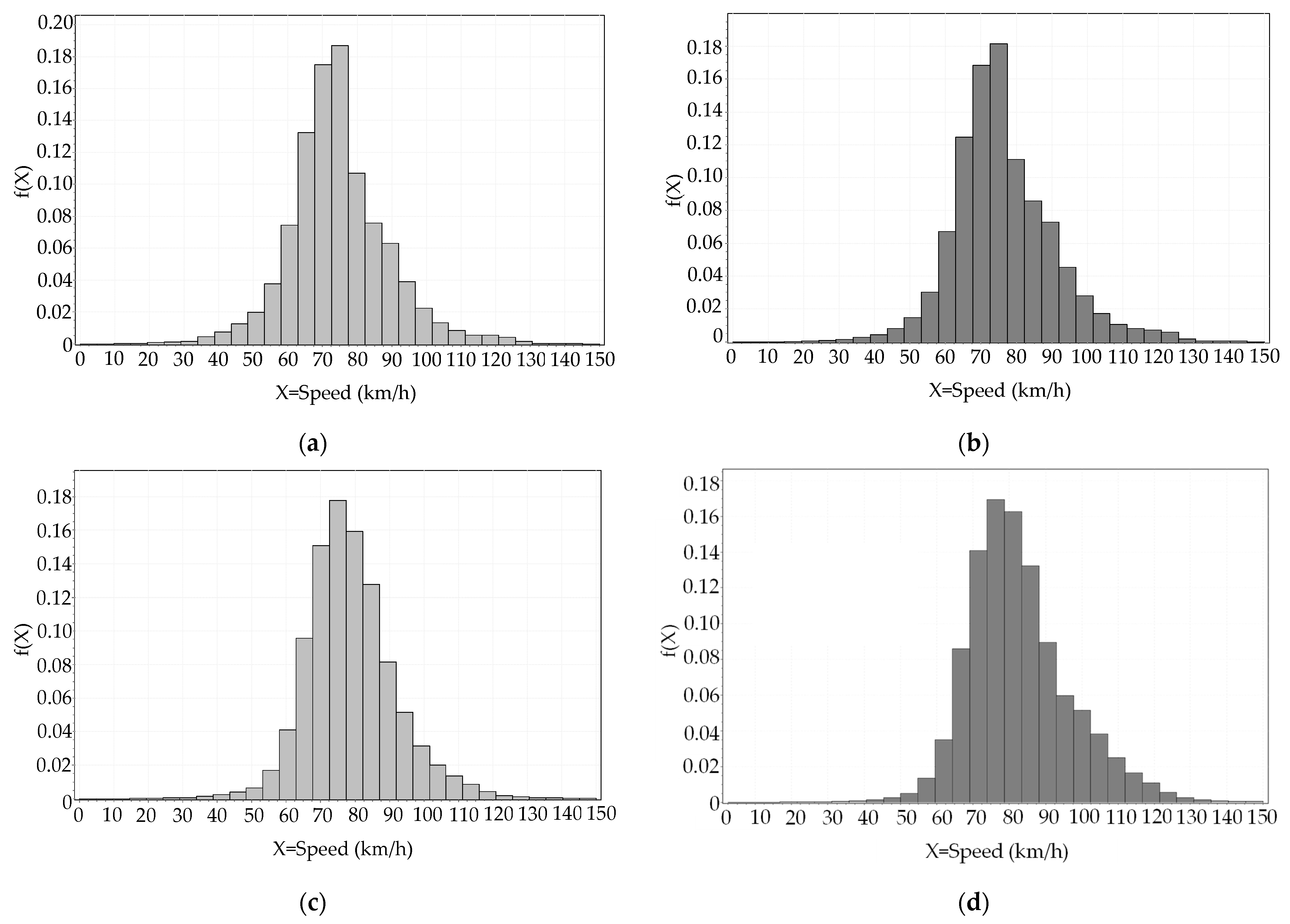
To validate the overall speed distribution across all virtual sections, the distribution obtained from the resampling process was compared to that from all original FV speed measurements. As illustrated by the histograms in Figure 5 and the descriptive statistics in Table 1, the probability distributions from the resampled 10-m VSs were consistent with the original FCD distributions. This confirmed that the smoothing splines effectively maintained the continuity and smoothness of individual vehicle speed tracks without distorting the original data.
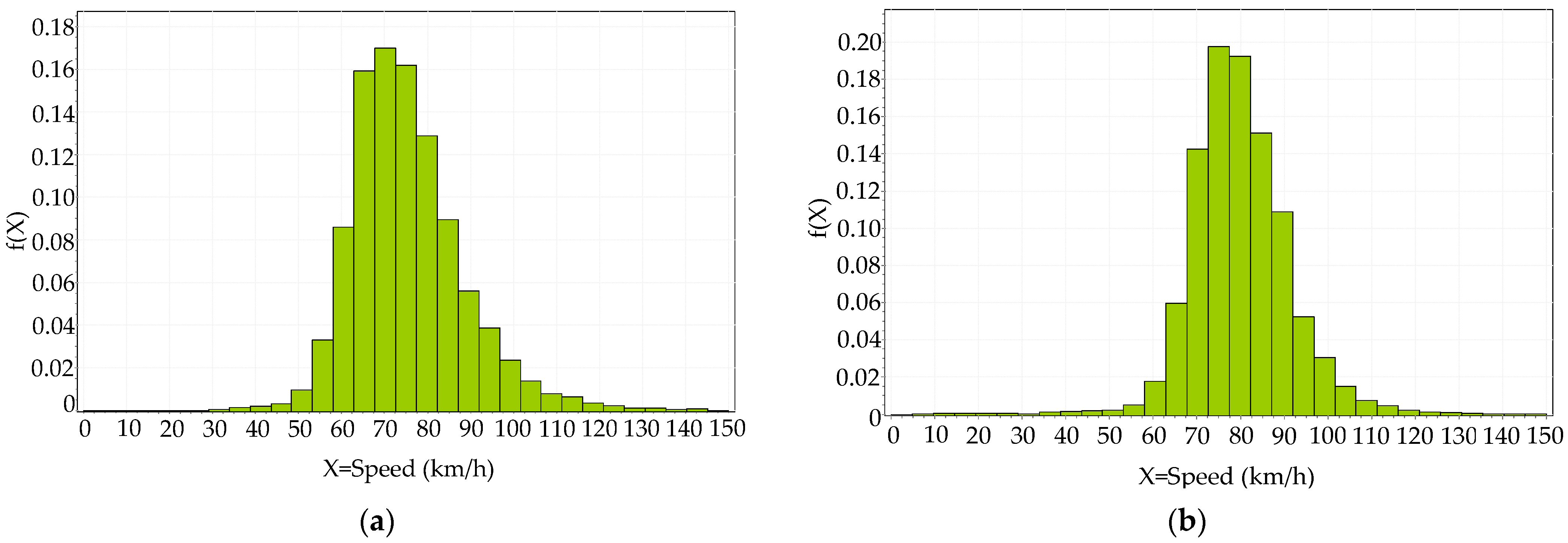
The SS14 highway segments 218 and 3191 are equipped with fixed monitoring devices (Control Units, CUs). The device on segment 218 is located at kilometer marker 17,085, while the device on segment 3191 is at kilometer marker 9047. Figure 6 illustrates the speed distributions of vehicles recorded by these devices, which operated continuously during three distinct periods: August 2018, February 2019, and May 2019.
Table 2 provides the descriptive statistics of the speeds detected in both travel directions. It is important to note that the Floating Car Data (FCD) for these segments pertains to the same monitoring periods.

5. Result and Discussion

With an extensive dataset of speed values recorded by the Control Units (CUs), the similarity between the probability distributions of these data and those from the Virtual Sections (VSs) can be assessed. Simply observing histograms or comparing descriptive statistics (Figure 5 and Figure 6, Table 1 and Table 2) does not provide a precise answer. Even with numerous statistics on centrality, dispersion, shape, symmetry, and percentiles, determining how closely the CU-sampled distributions match those sampled by mobile devices along the highway remains challenging.
To address this concisely, the 1-Wasserstein distance D 1 W P , Q can be used to measure the similarity between pairs of histograms P , Q . For histograms with congruent binning ( ϕ bins), the normalized 1-Wasserstein distance D 1 W ~ P , Q ranges from 0 (complete overlap and total similarity) to 1 (maximum dissimilarity).
Using the CU-recorded speed distribution q (histogram Q from Figure 6) as the reference, the similarity to any other distribution p can be measured by calculating D 1 W ~ P , Q . Table 3 presents the D 1 W ~ P , Q values for different segments and travel directions, with q representing CU data and p representing mobile sensor data.
Specifically, P 1 denotes the probability distribution p 1 from the entire resampled dataset in the VSs (Figure 5b,d) and P 2 represents p 2 , the resampled FCD data in the VSs near the CU. Consistent binning with ϕ = 3 1 bins is used, covering speed classes in 5 km/h intervals from 0 to 150 km/h plus an additional interval for speeds over 150 km/h.
The primary objective of this study is to analyze the evolution of speed distributions along highway segments, which has not been addressed thus far. Vehicular speed distributions may fluctuate due to varying conditions. To examine this variation, speed values in virtual sections along the two segments were considered, obtained by resampling speed values for each vehicle every 10 m using smoothing splines.
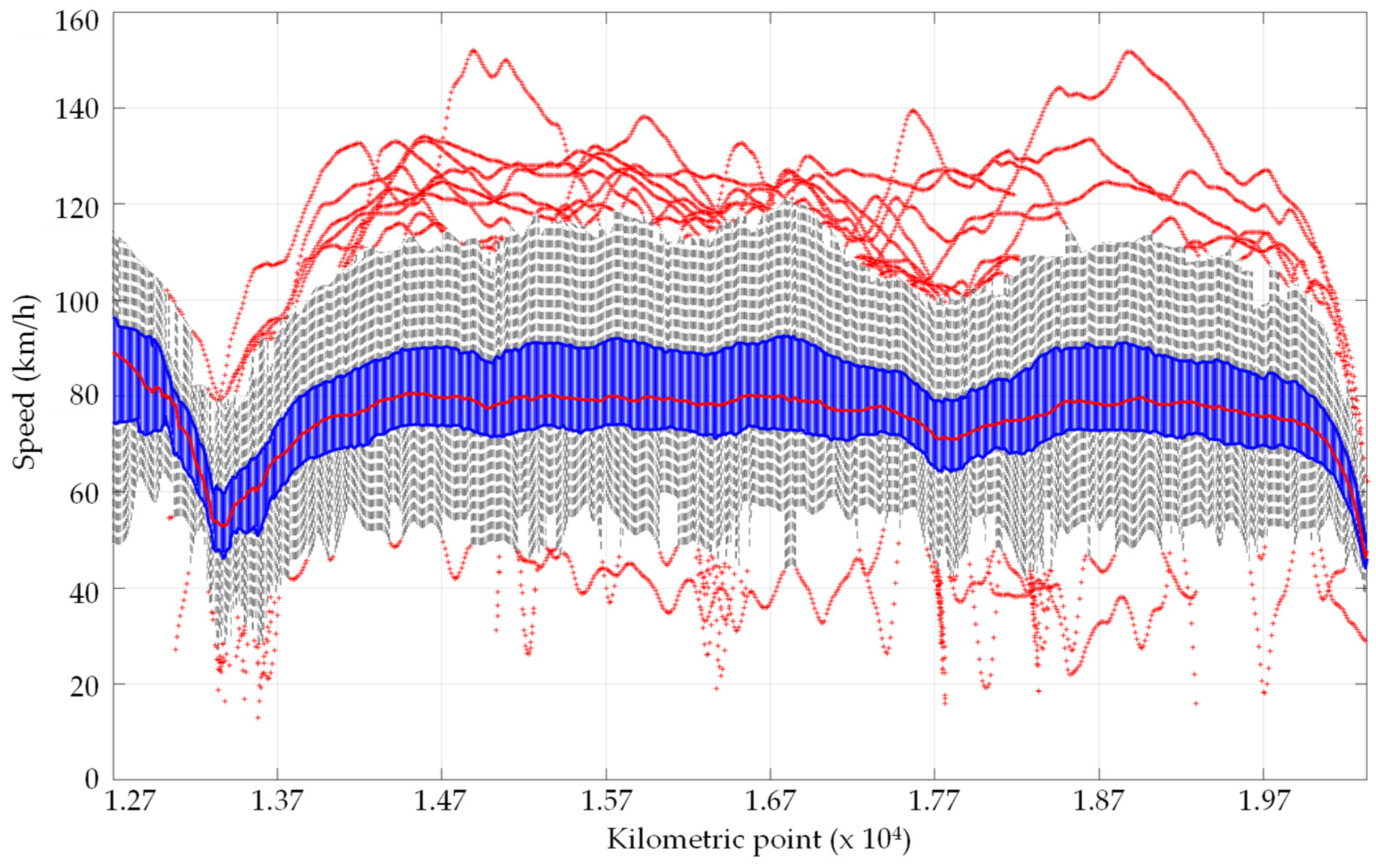
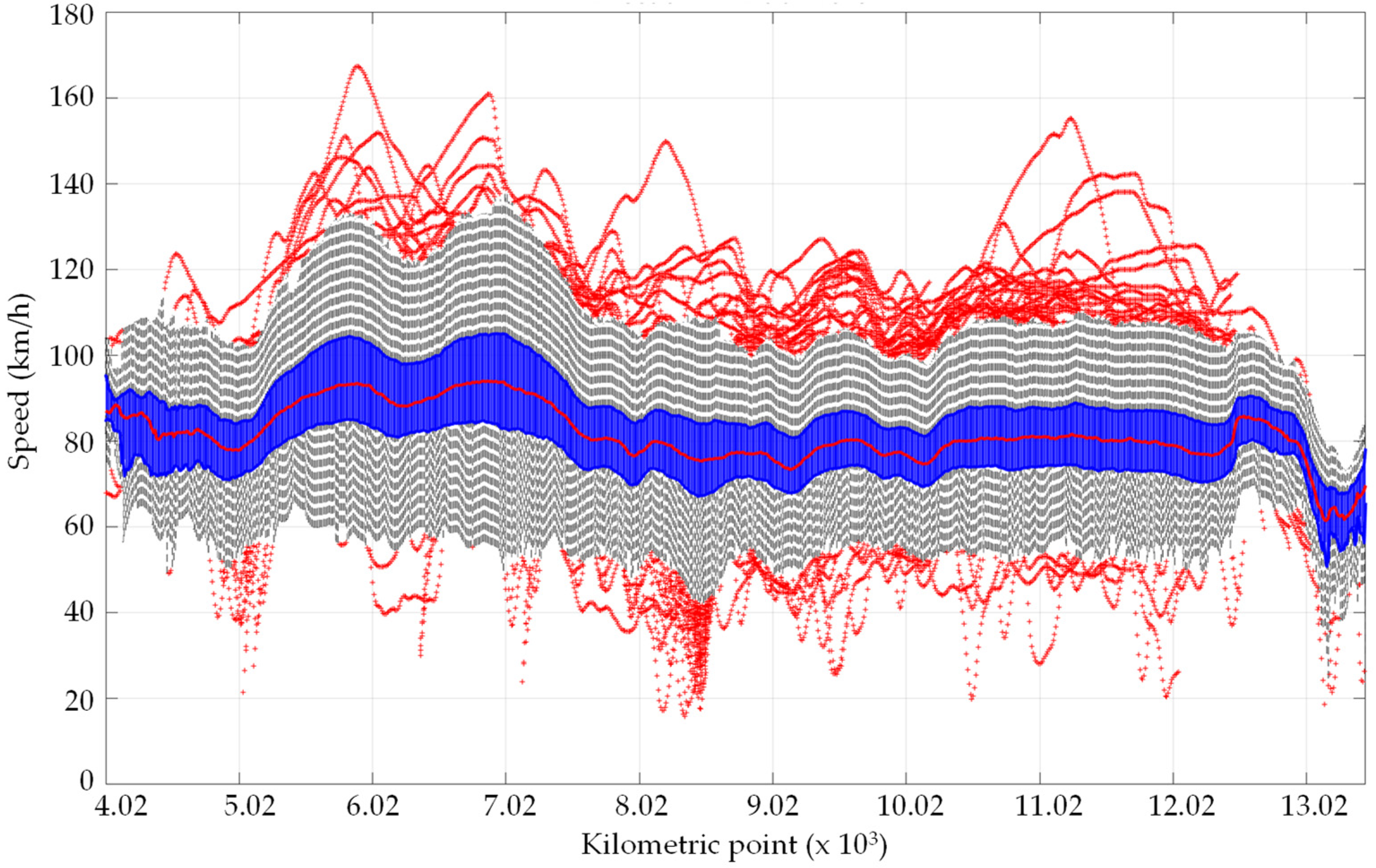
Figure 7 and Figure 8 present boxplots of speed data across these 10-m subsections. Each box represents the interquartile range (IQR) of speeds, with the median speed indicated by a line within the box. Whiskers extend to the furthest points within 1.5 times the IQR from the quartiles, and data beyond these whiskers are marked as outliers.
The blue band in the graphs represents the IQR, the continuous red line indicates the median, the dashed gray band shows the whiskers’ trend, and the pinpointed red values are outliers. The non-uniformity of the speed distribution among the different VSs can be inferred by observing the variability in the box plots as follows:
  • Box Length: Longer boxes indicate a wider range of speed values, so a variation in the box length suggests a variation in the range of speeds between sections;
  • Whisker Length: Longer whiskers show that there are more extreme speed values, so a variation in the whisker length between sections indicates a variation in the extreme speed values between them;
  • Position of the Median Line: A median line not centered within the box implies skewness in the data, indicating that the speed distribution is not symmetrical. Therefore, a variation in the position of the median line relative to the box between sections indicates a variation in the symmetry of the distribution among the sections;
  • Presence of Outliers: A higher number of outliers suggests more variability and potential anomalies in the speed distribution, so a variation in the outliers, in terms of number and position, indicates a variation in the values identified as anomalies among the different sections.
The boxplot series reveals significant variability across sections: median speeds fluctuate, indicating influences from factors such as road geometry, local traffic density, and differing regulations. Higher median speeds suggest road segments that permit or induce faster driving, while lower medians indicate areas with speed reductions due to geometry, interferences, lower speed limits, calming measures, or higher congestion. Thus, analyzing speed distribution variations requires considering the actual driving experiences of vehicles along the highway segment.
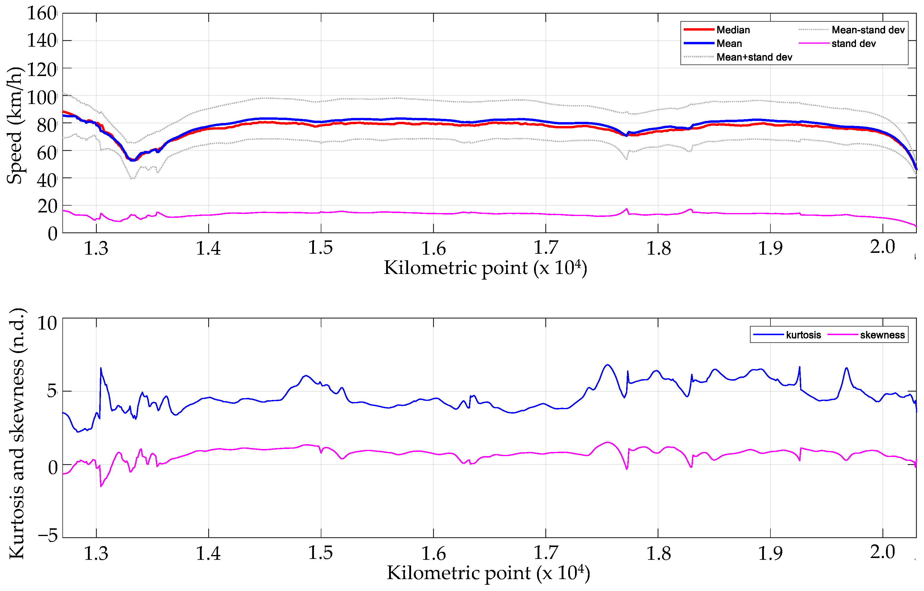
Thus, non-homogeneity in the speed distribution can be inferred by qualitatively observing the variability of the boxes and whiskers in the two boxplots. However, quantifying the dissimilarity in speed behaviors remains challenging. Figure 9 and Figure 10, which display trends of selected statistical values (including the mean, median, standard deviation, mean ± standard deviation, skewness, and kurtosis), also confirm this non-homogeneity in behavior. In Figure 9, both the median (red line) and mean (blue line) exhibit noticeable drops between 1.3 and 1.4 × 10⁴ km, between 1.78 and 1.83 × 10⁴ km, and over 2.0 × 10⁴ km, reflecting significant changes in central speed values. Additional fluctuations along the x-axis indicate variability in driving behavior. The standard deviation (pink line) shows substantial variations in the same locations, highlighting increased speed dispersion in these sections. The mean ± standard deviation (gray lines) further emphasizes changes in speed distribution around the mean at these key points. Skewness (pink line) is generally close to zero but deviates around the key points and in other virtual sections along the axis, suggesting occasional asymmetry in speed distribution. Kurtosis (blue line) shows significant changes, especially coinciding with skewness variations, indicating variations in the peakedness of the speed distribution with more extreme values present in sections with high values.
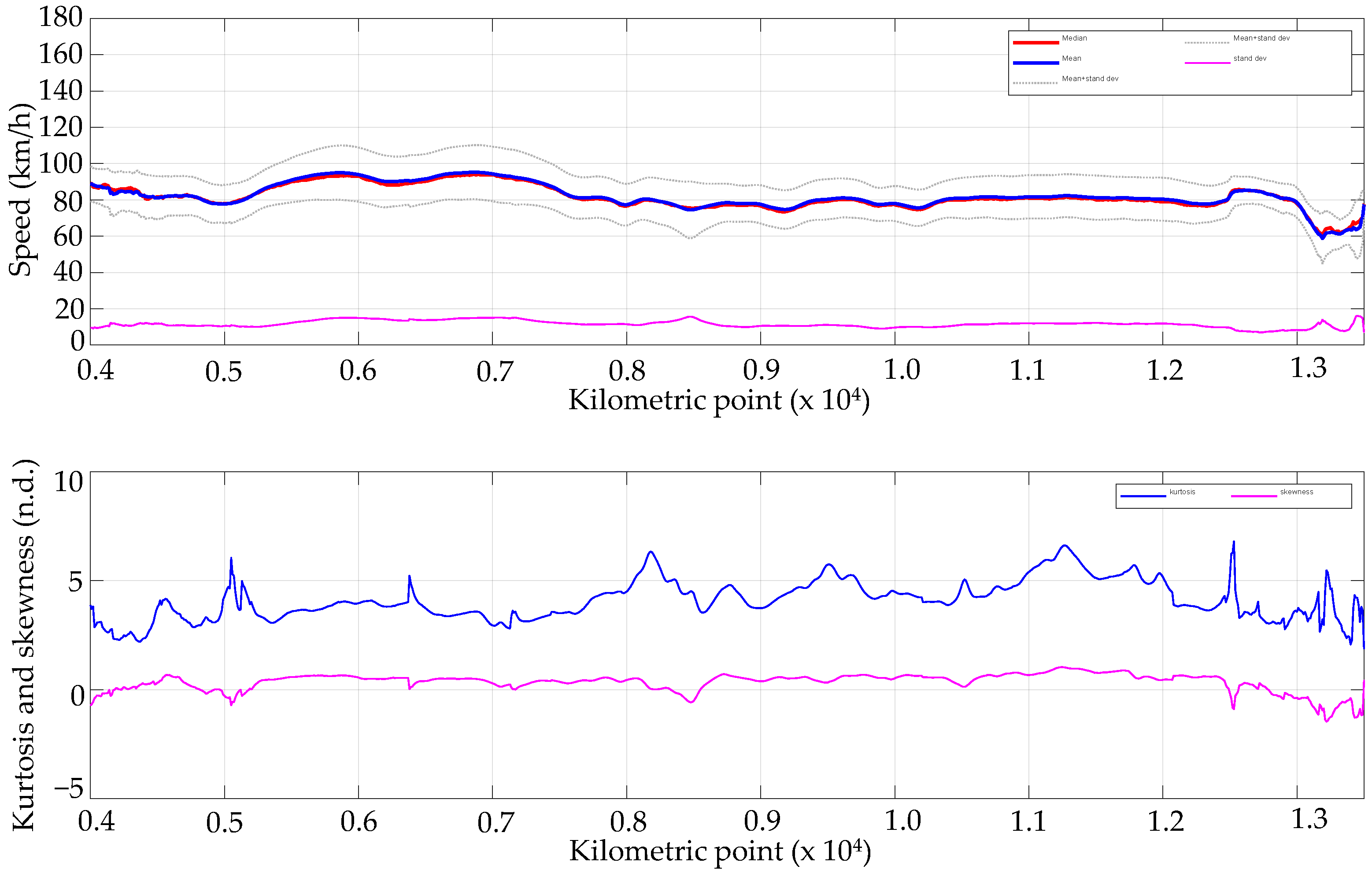
Similar considerations can be made by examining the trends in Figure 10. The median (red line) and mean (blue line) display notable fluctuations along the segment, especially around 0.53–0.74 × 10⁴ km, signifying significant changes in central speed values. The standard deviation (pink line) exhibits marked increases at these same points, highlighting greater speed dispersion and variability in these sections. The mean ± standard deviation (gray lines) underscores these changes, illustrating how speed values spread out from the mean. Skewness (pink line) tends to stay close to zero but shows deviations, indicating that the speed distribution sometimes shifts asymmetrically. Kurtosis (blue line) displays notable peaks and troughs, especially where skewness changes, signifying variations in the peakedness of the speed distribution.
Although various statistical indices are available to examine different aspects of the experimental distributions, there is no effective synthesis method for determining homogeneity from the perspective of the probabilistic distribution of speeds.
In this context, the normalized 1-Wasserstein distance D 1 W ~ P , Q can be used to measure the similarity of the speed distribution along the two road segments considered as examples.
Figure 11 shows the trend of the series of histograms aggregated with ϕ = 3 1 bins (speed classes in 5 km/h intervals from 0 to 150 km/h plus an additional interval for speeds over 150 km/h) that represent the vehicular speed distribution trends in the different VSs identified in the two segments, 218 DISC and 3191 ASC.
Having already confirmed the strong similarity between the CU-recorded speed distribution q and the speed distribution p 2 from resampled FCD data in the VSs near the CU, the histogram P 2 representing the distribution p 2 can be assumed as a benchmark for the similarity analysis of the highway segment. Consequently, the normalized 1-Wasserstein distance D 1 W ~ D x , P 2 is determined, signifying the variation in speed histograms D x (with x changing as the VS progresses) compared to the histogram in the VS close to the CU location along the entire length of the highway segment.
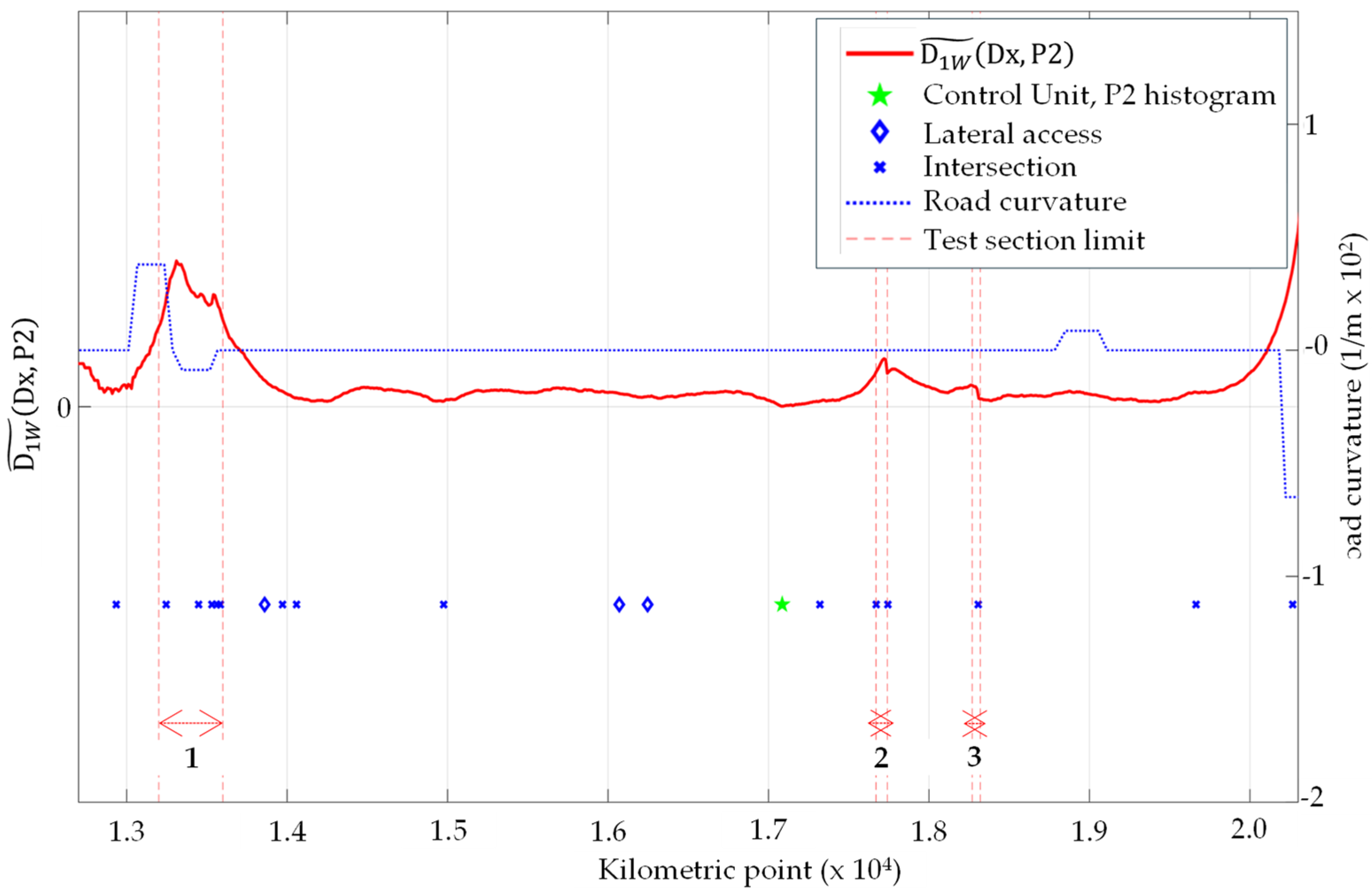
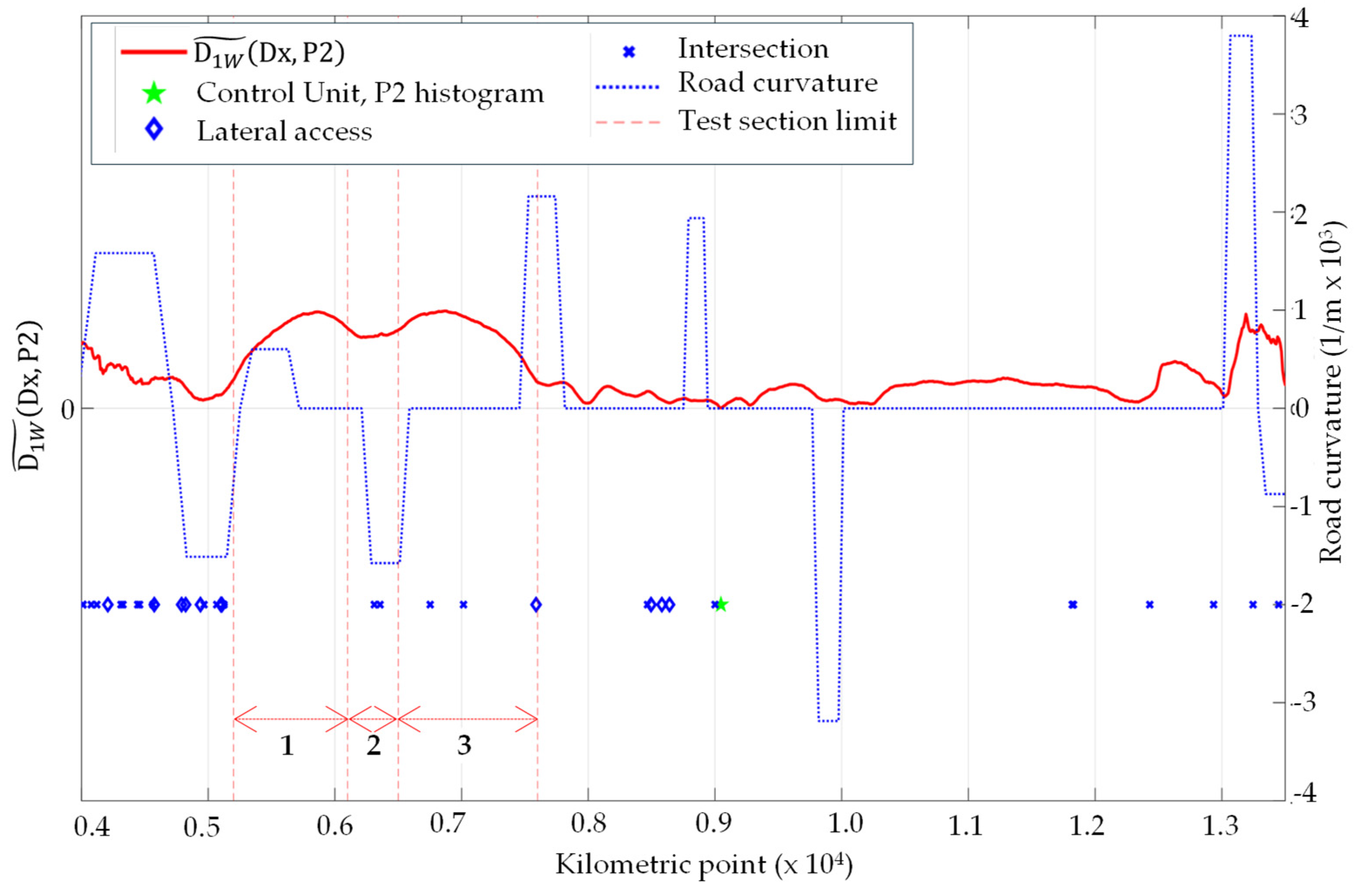
Figure 12 and Figure 13 describe the segment features in terms of road geometry and the surrounding context. The variable D 1 W ~ D x , P 2 was superimposed on the same graph with the curvature diagram to assess the influence of winding elements. The curvature trend was calculated using the radius R x of the curvature of the highway axis at a given point ( x ) by the formula K x = 1/ R x . The graphs also show the positions along the curvilinear abscissa of various elements such as intersections and access to private and public areas [56]. Additionally, each segment includes the localization of the CU as a reference term. The symbols explained in the legend (blue cross symbol for Intersections, blue diamond symbol for Lateral accesses, and green star for Control units) are positioned along the x-axis based on their locations along the kilometric distances.
Examining the graph in Figure 12, which pertains to segment 218 DISC, it is evident that the red line D 1 W ~ D x , P 2 exhibits significant peaks at points where the curvature is more pronounced, specifically around 1.33, and 2.02 × 10⁴ km. These peaks indicate that changes in road curvature have a considerable impact on the similarity of speed distributions. Sharp curves tend to cause variations in driving behavior, which in turn affects the similarity between speed distributions in these areas compared to the reference section.
Throughout the segment, lateral access points and intersections are scattered. Although lateral access points do not show a strong correlation with the peaks or troughs in the red line, intersections sometimes cause slight fluctuations. This suggests that intersections introduce minor disruptions to speed consistency, but their impact is not as significant as road curvature. The flatter portions of the red line, between 1.4 and 1.7 × 10⁴ km, correspond to sections with fewer intersections and lateral accesses, coupled with relatively stable road curvature. In these segments, the speed distribution aligns more closely with the reference section, indicating that less complex road geometry and fewer interruptions contribute to higher similarity in speed distributions.
Turning to the graph in Figure 13, related to segment 3191 ASC, the red line D 1 W ~ D x , P 2 shows significant peaks at points of high road curvature and near lateral accesses and intersections. Between 0.5 and 0.8 × 10⁴ km, where the road is widened, the red line exhibits notable fluctuations, suggesting that changes in road width significantly impact the speed distribution. Similarly, regions with straight road segments and the absence of lateral accesses and intersections present the greatest similarity with the reference section. These areas likely allow for more uniform driving speeds, enhancing the similarity in speed distributions.
Following the analysis of the graphs in Figure 12 and Figure 13, the Table 4 provides a numerical summary of the average normalized 1-Wasserstein distance for specific sub-segments. Segment 218 (DESC direction) and segment 3191 (ASC direction) are evaluated at three distinct test sub-segments each, and the average values highlight the variability in speed distribution similarity. These numerical insights provide a quantitative perspective on how various road features influence the similarity of speed distributions, complementing the visual analysis from the graphs.
Overall, D 1 W ~ D x , P 2 tends to peak at points where there are significant changes in road curvature, road widening, lateral accesses, and intersections. This pattern indicates that these factors are crucial in influencing the homogeneity of speed probability distributions along the road segment. The analysis highlights the critical role of road geometry in shaping speed distribution probability. Sharp curves and high curvature areas consistently disrupt speed patterns, suggesting that road design must account for these features to maintain consistent driving behavior.
Intersections, while causing slight fluctuations, have a less significant impact compared to road curvature. Lateral access points also introduce some variability in speed distributions, though their effect is minimal. The widening of the road, as seen in segment 3191 ASC, significantly impacts speed distributions, suggesting that road widening projects need to consider the potential for increased variability in driving behavior, which can affect overall traffic flow and safety. Regions with straight road segments and fewer interruptions (intersections and accesses) exhibit the highest homogeneity in speed distributions. This implies that simpler road designs may contribute to more uniform driving speeds, potentially enhancing traffic efficiency and safety [57].

Future Developments of the Research

As we have seen in Section 3.4, D 1 W p , q can be easily visualized as the area between two CDFs, F p and F q . Considering p = 2 with the Euclidean norm in Equation (4), the 2 -Wasserstein ( 2 W) distance D 2 W p , q can be defined, also known as the Fréchet distance [49]:
D 2 W p , q = 0 1 F p 1 s F q 1 s 2 d s 1 2
Arroyo and Maté [34] and Balzanella and Irpino [23] provide the explicit form for D 2 W P , Q for histograms P and Q . Irpino and Romano [58] show a particularly useful property of the D 2 W demonstrating the equivalence with a three-term decomposition using the differences between statistics of the two distributions: location, spread, and shape. In fact, the squared value D 2 W 2 , a natural extension of the Euclidean distance from point data to distribution data [59], can be decomposed as the sum of the square difference of the means (i.e., location), the square difference of the standard deviations (i.e., spread) and a residual term, which can be assumed to represent a shape distance between two distributions.
D 2 W 2 = 0 1 F p 1 s F q 1 s 2 d s = μ p μ q 2 + σ p σ q 2 + 2 σ p σ q 1 C o r r p q
where μ p and μ q are the mean of p and q and σ p and σ q are the standard deviation of p and q . C o r r p q is the Pearson correlation of the points in the Quantile-Quantile plot of F p and F q .
C o r r p q = 0 1 F p 1 s μ p F q 1 s μ q d s σ p σ q
Thus, these three terms can be used to assess similarity/dissimilarity between p and q in a useful and distinctive manner regarding location, spread, and shape differences.
Moreover, when F p and F q are not explicitly given, as for experimental distributions represented as step functions (commonly seen in similarity/dissimilarity analysis of vehicle speed distributions along a road axis), the measurement of similarity according to the Wasserstein distance can be carried out. This avoids the need to represent experimental distribution functions as histograms, which involves challenges such as choosing an appropriate origin and the number of bins. However, for p = 2 , the three-term decomposition allows us to directly represent the square of the Wasserstein distance using the empirical versions of the corresponding quantities in Equation (7).
These aspects related to the 2-Wasserstein distance and its representation through decomposition are suggested as points for further investigation. They can be explored in future research activities and application tests, aiming to achieve an effective representation of the homogeneity or heterogeneity of speed distribution along rural highway segments.

6. Conclusions

This study delves into the analysis of the heterogeneity in speed distributions along secondary rural road segments using Floating Car Data (FCD) and data from fixed control stations. The goal is to provide a useful tool to better understand how physical and geometric characteristics of roads influence speed behavior, which is crucial for road safety and traffic management. The presence of at-grade intersections that handle significant traffic volumes necessitates the inclusion of specialized lanes, such as left-turn lanes. These features likely contribute to more consistent speeds due to the structured flow of traffic and the availability of dedicated lanes for turning movements. A reduced lane width and the absence of specialized lanes can lead to greater variability in speed distribution as vehicles may need to adjust their speeds more frequently due to the presence of direct access points and narrower lanes.
This study highlights the benefits of using advanced similarity measures to capture the variability and heterogeneity in traffic speed distributions. These measures facilitate a more comprehensive analysis of traffic patterns, which is essential for informed highway design, performance and safety verification, and regulatory compliance.
To achieve this, continuous speed and location data were collected from GPS-equipped vehicles (FCD) and validated against radar control units. The normalized 1-Wasserstein distance, a non-parametric similarity measure, was employed to compare speed distributions in virtual sections placed at 10-m intervals along the road. In each virtual section, vehicle speeds were obtained by resampling the smoothing splines that reconstruct the speed-position profiles of each equipped vehicle. The findings demonstrate that the normalized 1-Wasserstein distance effectively captures speed distribution variability. This allows for a detailed examination of how road features, such as curvature, intersections, and access points, influence speed behavior. By utilizing the normalized 1-Wasserstein distance, the analysis provides a concise and effective metric for evaluating speed distribution similarities across various road segments. This approach offers a more comprehensive analysis than traditional summary statistics or representations.
Overall, the findings underscore the potential of these techniques to enhance traffic management strategies and improve road safety by providing a deeper insight into the dynamics of vehicular speeds across different road environments. The practical implications of this research are significant, as the application of the normalized 1-Wasserstein distance can directly inform road safety measures, traffic regulation policies, and the design of more effective traffic management systems.
Furthermore, the study proposes the future exploration of the application of the Wasserstein distance with the Euclidean L2 norm. This approach decomposes the measure into three key dimensions: mean (location), variance (spread), and correlation (shape) of the experimental distributions. Continued research utilizing this decomposition could provide a more detailed assessment of dissimilarity, moving beyond simple histogram characterization to provide a more refined understanding of the differences in speed distributions.

Author Contributions

Conceptualization, G.C. and R.M.; methodology, A.P.; software, A.P. and P.P.; validation, G.D.S.; formal analysis, R.M.; investigation, G.D.S.; resources, G.C.; data curation, P.P.; writing—original draft preparation, A.P.; writing—review and editing, G.D.S.; visualization, P.P.; supervision, R.M.; project administration, G.C. All authors have read and agreed to the published version of the manuscript.

Funding

This research received no external funding.

Institutional Review Board Statement

Not applicable.

Informed Consent Statement

Not applicable.

Data Availability Statement

The original contributions presented in the study are included in the article, further inquiries can be directed to the corresponding author.

Conflicts of Interest

The authors declare no conflict of interest.

References

  1. Apostoleris, K.A.; Sarma, S.N.; Antonios, T.E.; Basil, P. Traffic speed variability as an indicator of the provided road safety level in two-lane rural highways. Transp. Res. Procedia 2023, 69, 241–248. [Google Scholar] [CrossRef]
  2. Del Serrone, G.; Cantisani, G.; Peluso, P. Speed data collection methods: A review. Transp. Res. Procedia 2023, 69, 512–519. [Google Scholar] [CrossRef]
  3. Treiber, M.; Helbing, D. Reconstructing the spatio-temporal traffic dynamics from stationary detector data. Coop. Transp. Dyn. 2002, 1, 3–24. [Google Scholar]
  4. Herty, M.; Tosin, A.; Visconti, G.; Zanella, M. Reconstruction of traffic speed distributions from kinetic models with uncertainties. In Mathematical Descriptions of Traffic Flow: Micro, Macro and Kinetic Models; Tosin, A., Puppo, G., Eds.; Springer: Berlin/Heidelberg, Germany, 2019. [Google Scholar] [CrossRef]
  5. Li, J.; Perrine, K.; Wu, L.; Walton, C.M. Cross-validating traffic speed measurements from probe and stationary sensors through state reconstruction. Int. J. Transp. Sci. Technol. 2019, 8, 290–303. [Google Scholar] [CrossRef]
  6. Cantisani, G.; Del Serrone, G.; Peluso, P. Reliability of Historical Car Data for Operating Speed Analysis along Road Networks. Sci 2022, 4, 18. [Google Scholar] [CrossRef]
  7. Altintasi, O.; Tuydes-Yaman, H.; Tuncay, K. Quality of floating car data (FCD) as a surrogate measure for urban arterial speed. Can. J. Civ. Eng. 2019, 46, 1187–1198. [Google Scholar] [CrossRef]
  8. Budimir, D.; Jelušić, N.; Perić, M. Floating Car Data Technology. Pomorstvo 2019, 33, 22–32. [Google Scholar] [CrossRef]
  9. Ambros, J.; Gogolín, O.; Kubeček, J.; Andrášik, R.; Bíl, M. Proactive identification of risk road locations using vehicle fleet data: Exploratory study. In Proceedings of the 28th ICTCT Workshop, Ashod, Israel, 29–30 October 2015; pp. 29–30. [Google Scholar]
  10. Fabrizi, V.; Ragona, R. A pattern matching approach to speed forecasting of traffic networks. Eur. Transp. Res. Rev. 2014, 6, 333–342. [Google Scholar] [CrossRef]
  11. Zhang, J.B.; Song, G.H.; Yu, L.; Guo, J.F.; Lu, H.Y. Identification and characteristics analysis of bottlenecks on urban expressways based on floating car data. J. Cent. South Univ. 2018, 25, 2014–2024. [Google Scholar] [CrossRef]
  12. Mehrabani, B.B.; Mirbaha, B. Evaluating the relationship between operating speed and collision frequency of rural multilane highways based on geometric and roadside features. Civ. Eng. J. 2018, 4, 609. [Google Scholar] [CrossRef]
  13. Gheorghiu, R.A.; Iordache, V.; Stan, V.A. Urban traffic detectors—Comparison between inductive loop and magnetic sensors. In Proceedings of the International Conference on Electronics, Computers and Artificial Intelligence (ECAI), Pitesti, Romania, 29–30 June 2021. [Google Scholar] [CrossRef]
  14. Agresti, A.; Franklin, C.; Klingenberg, B. Statistics: The Art and Science of Learning from Data, Global Edition, 4th ed.; Pearson Education: London, UK, 2023; ISBN 9781292442464. [Google Scholar]
  15. Nahm, F.S. Nonparametric statistical tests for the continuous data: The basic concept and the practical use. Korean J. Anesthesiol. 2016, 69, 8–14. [Google Scholar] [CrossRef]
  16. Provost, F.; Fawcett, T. Data Science for Business: What You Need to Know about Data Mining and Data-Analytic Thinking; O’Reilly Media: Sebastopol, CA, USA, 2013; ISBN 978-1-449-36132-7. [Google Scholar]
  17. Hastie, T.; Tibshirani, R.; Friedman, J. The Elements of Statistical Learning: Data Mining, Inference, and Prediction, 2nd ed.; Springer: New York, NY, USA, 2008. [Google Scholar]
  18. Murphy, K.P. Introduction. In Machine Learning a Probabilistic Perspective, 1st ed.; MIT Press: London, UK, 2012; pp. 1–2. [Google Scholar]
  19. Mathisen, B.M.; Aamodt, A.; Bach, K.; Langseth, H. Learning similarity measures from data. Prog. Artif. Intell. 2020, 9, 129–143. [Google Scholar] [CrossRef]
  20. Sammut, C.; Webb, G.I. Encyclopedia of Machine Learning and Data Mining; Springer Publishing Company, Incorporated: Berlin/Heidelberg, Germany, 2017. [Google Scholar]
  21. Bishop, C.M. Pattern Recognition and Machine Learning (Information Science and Statistics); Springer: Berlin/Heidelberg, Germany, 2006. [Google Scholar]
  22. Aggarwal, C.C.; Reddy, C.K. Data Clustering Algorithms and Applications, 1st ed.; CRC Press: Boca Raton, FL, USA, 2013; pp. 65–210. [Google Scholar]
  23. Balzanella, A.; Irpino, A. Spatial prediction and spatial dependence monitoring on georeferenced data streams. Stat. Methods Appl. 2020, 29, 101–128. [Google Scholar] [CrossRef]
  24. Sulewski, P. Equal-bin-width histogram versus equal-bin-count histogram. J. Appl. Stat. 2021, 48, 2092–2111. [Google Scholar] [CrossRef]
  25. Qian, X.; Cabanes, G.; Rastin, P.; Guidani, M.A.; Marrakchi, G.; Clausel, M.; Grozavu, N. An Innovative Framework for Static and Dynamic Clustering Using Histogram Models and Wasserstein Distance Over Sliding Windows. SSRN 2023. Available online: https://ssrn.com/abstract=4573414 (accessed on 1 July 2024).
  26. Billard, L.; Diday, E. From the statistics of data to the statistics of knowledge: Symbolic data analysis. J. Am. Stat. Assoc. 2003, 98, 470–487. [Google Scholar] [CrossRef]
  27. Silverman, B.W. Density Estimation for Statistics and Data Analysis; Monographs on Statistics and Applied Probability; Chapman and Hall: London, UK, 1986; Includes Bibliographical References; pp. 59–165. [Google Scholar] [CrossRef]
  28. Dekking, F.; Kraaikamp, C.; Lopuhaä, H. A Modern Introduction to Probability and Statistics: Understanding Why and How; Springer: London, UK, 2005. [Google Scholar]
  29. Pearson, K. Contributions to the mathematical theory of evolution. Philos. Trans. R. Soc. Lond. A 1894, 185, 71–110. [Google Scholar] [CrossRef]
  30. Scott, D.W. On Optimal and Data-Based Histograms. Biometrika 1979, 66, 605–610. [Google Scholar] [CrossRef]
  31. Freedman, D.; Diaconis, P. On the histogram as a density estimator: L2 theory. Z. FüR Wahrscheinlichkeitstheorie Und Verwandte Geb. 1981, 57, 453–476. [Google Scholar] [CrossRef]
  32. Mosteller, F.; Tukey, J. Data Analysis and Regression: A Second Course in Statistics, 1st ed.; Pearson: Reading, MA, USA, 1977; ISBN 978-0-201-04854-4. [Google Scholar]
  33. Arroyo, J.; Maté, C. Forecasting histogram time series with k-nearest neighbours methods. Int. J. Forecast. 2009, 25, 192–207. [Google Scholar] [CrossRef]
  34. Billard, L.; Diday, E. Symbolic Data Analysis: Conceptual Statistics and Data Mining; John Wiley & Sons, Ltd.: Hoboken, NJ, USA, 2007. [Google Scholar]
  35. Strelkov, V.V. A new similarity measure for histogram comparison and its application in time series analysis. Pattern Recognit. Lett. 2008, 29, 1768–1774. [Google Scholar] [CrossRef]
  36. Shnoll, S.E.; Kolombet, V.A.; Pozharskii, E.V.; Zenchenko, T.A.; Zvereva, I.M.; Konradov, A.A. On discrete states due to macroscopic fluctuations. Uspekhi Fizicheskikh Nauk 1998, 168, 1129–1140. [Google Scholar] [CrossRef]
  37. Shnoll, S.E.; Pozharski, E.V.; Zenchenko, T.A.; Kolombet, V.A.; Zvereva, I.M.; Konradov, A.A. Fine structure of distributions in measurements of different processes as affected by geophysical and cosmophysical factors. Phys. Chem. Earth Part A Solid Earth Geod. 1999, 24, 711–714. [Google Scholar] [CrossRef]
  38. Fedorov, M.V.; Belousov, L.V.; Voeikov, V.L.; Zenchenko, T.A.; Zenchenko, K.I.; Pozharskii, E.V.; Konradov, A.A.; Shnoll, S.E. Synchronous changes in dark current fluctuations in two separate photomultipliers in relation to Earth rotation. Astrophys. Space Sci. 2003, 283, 3–10. [Google Scholar] [CrossRef]
  39. Magyar, J.C.; Sambridge, M. Hydrological objective functions and ensemble averaging with the Wasserstein distance. Hydrol. Earth Syst. Sci. 2023, 27, 991–1010. [Google Scholar] [CrossRef]
  40. Lee, T.; Xiao, Y.; Meng, X.; Duling, D. Clustering Time Series Based on Forecast Distributions Using Kullback-Leibler Divergence. International Institute of Forecasters (IIF). 2014. Available online: https://forecasters.org/wp-content/uploads/gravity_forms/7-2a51b93047891f1ec3608bdbd77ca58d/2013/06/ISF2013_LEE_TSClustering.pdf (accessed on 1 July 2024).
  41. Ma, Y.; Gu, X.; Wang, Y. Histogram similarity measure using variable bin size distance. Comput. Vis. Image Underst. 2010, 114, 981–989. [Google Scholar] [CrossRef]
  42. Rubner, Y.; Tomasi, C.; Guibas, L.J. The Earth Mover’s Distance as a metric for image retrieval. Int. J. Comput. Vis. 2000, 40, 99–121. [Google Scholar] [CrossRef]
  43. Bazan, E.; Dokládal, P.; Dokladalova, E. Quantitative analysis of similarity measures of distributions. In Proceedings of the British Machine Vision Conference, Cardiff, UK, 9–12 September 2019; p. 187. [Google Scholar]
  44. Bellemare, M.G.; Danihelka, I.; Dabney, W.; Mohamed, S.; Lakshminarayanan, B.; Hoyer, S.; Munos, R. The Cramer distance as a solution to biased Wasserstein gradients. arXiv. 2017. Available online: https://arxiv.org/abs/1705.10743 (accessed on 1 July 2024).
  45. Khamsi, M.A. Generalized metric spaces: A survey. J. Fixed Point Theory Appl. 2015, 17, 455–475. [Google Scholar] [CrossRef]
  46. Kantorovich, L.V. On the translocation of masses. Dokl. Akad. Nauk 1942, 37, 227–229. [Google Scholar] [CrossRef]
  47. Dobrushin, R.L. Prescribing a System of Random Variables by Conditional Distributions. Theory Probab. Its Appl. 1970, 15, 458–486. [Google Scholar] [CrossRef]
  48. Vaseršteĭn, L.N. Markov processes over denumerable products of spaces, describing large systems of automata. Probl. Peredači Inf. 1969, 5, 64–72. [Google Scholar]
  49. Monge, G. Mémoire sur la théorie des déblais et des remblais. In Histoire de l’Académie Royale des Sciences de Paris; De l’Imprimerie Royale: Paris, France, 1781. [Google Scholar]
  50. Panaretos, V.M.; Zemel, Y. Statistical aspects of Wasserstein distances. Annu. Rev. Stat. Appl. 2019, 6, 405–431. [Google Scholar] [CrossRef]
  51. Dall’Aglio, G. Sugli estremi dei momenti delle funzioni di ripartizione doppia. Ann. Della Sc. Norm. Super. Pisa Cl. Sci. 1956, 10, 35–74. [Google Scholar]
  52. Ramdas, A.; Trillos, N.G.; Cuturi, M. On Wasserstein two-sample testing and related families of nonparametric tests. Entropy 2017, 19, 47. [Google Scholar] [CrossRef]
  53. Levina, E.; Bickel, P.J. The earth mover’s distance is the Mallows distance: Some insights from statistics. In Proceedings of the Eighth IEEE International Conference on Computer Vision, ICCV 2001, Vancouver, BC, Canada, 7–14 July 2001; Volume 2, pp. 251–256. [Google Scholar]
  54. Santambrogio, F. Optimal transport for applied mathematicians. Birkäuser 2015, 55, 94. [Google Scholar] [CrossRef]
  55. Andrieu, C.; Saint Pierre, G.; Bressaud, X. Estimation of Space-Speed Profiles: A Functional Approach Using Smoothing Splines. In Proceedings of the 2013 IEEE Intelligent Vehicles Symposium (IV), Gold Coast, Australia, 23–26 June 2013; pp. 982–987. [Google Scholar]
  56. Cantisani, G.; Del Serrone, G. Procedure for the identification of existing roads alignment from georeferenced points database. Infrastructures 2021, 6, 2. [Google Scholar] [CrossRef]
  57. Del Serrone, G.; Cantisani, G.; Peluso, P.; Coppa, I.; Mancinetti, M.; Bianchini, B. Road infrastructure safety management: Proactive safety tools to evaluate potential conditions of risk. Transp. Res. Procedia 2023, 69, 711–718. [Google Scholar] [CrossRef]
  58. Irpino, A.; Romano, E. Optimal histogram representation of large data sets: Fisher vs piecewise linear approximations. Rev. Des Nouv. Technol. De L’information 2007, 1, 99–110. [Google Scholar]
  59. Košmelj, K.; Billard, L. Mallows’ L2 distance in some multivariate methods and its application to histogram-type data. J. Adv. Stat. 2012, 9, 107–118. [Google Scholar] [CrossRef]
Figure 1. (a) Monge’s formulation of OT, with a source mass distribution (light green) and a target to be filled (light blue); (b) solution of the OT problem, with the transport map (black line) and the transport for a particular point from the source distribution to the target distribution.
Sci 06 00052 g001
Figure 2. Empirical cumulative distribution functions (ECDFs) F p and F q , intuition of 1-Wasserstein distance, i.e., the total area between the two ECDFs (shaded) and the Kolmogorov–Smirnov (KS) distance, i.e., the maximum distance between the two ECDFs (double-headed arrow).
Sci 06 00052 g002
Figure 3. Smoothing splines restricted to the virtual sections that included a minimum of 10 vehicles: segment 218 (from km 12,660 to km 20,310 with travel direction DESC); the different colored lines indicate individual vehicles smoothing splines.
Sci 06 00052 g003
Figure 4. Smoothing splines restricted to the virtual sections that included a minimum of 10 vehicles: segment 3191 (from km 4000 to km 13,470 with travel direction ASC); the different colored lines indicate individual vehicles smoothing splines.
Sci 06 00052 g004
Figure 5. Histograms for speed distribution: (a) original FCD for segment 218; (b) virtual section by smoothing splines for segment 218; (c) original FCD for segment 3191; and (d) virtual section by smoothing splines for segment 3191.
Sci 06 00052 g005
Figure 6. Histograms for speed distribution from CUs: (a) segment 218 and (b) segment 3191.
Sci 06 00052 g006
Figure 7. Boxplot analysis of speed distributions at 10-m intervals in VSs along segment 218 (DESC direction).
Sci 06 00052 g007
Figure 8. Boxplot analysis of speed distributions at 10-m intervals in VSs along segment 3191 (ASC direction).
Sci 06 00052 g008
Figure 9. Trends of selected statistical values for the experimental speed distributions in VSs along the segment 218 DESC.
Sci 06 00052 g009
Figure 10. Trends of selected statistical values for the experimental speed distributions in VSs along the segment 3191 ASC.
Sci 06 00052 g010
Figure 11. Three-dimensional histogram series of speeds in VSs: (a) segment 218 DESC and (b) segment 3191 ASC.
Sci 06 00052 g011
Figure 12. D 1 W ~ D x , P 2 along the segment 281 DISC and segment features representation; sub-sections 1, 2, and 3 identify the histograms of the speed distributions D1, D2, and D3.
Sci 06 00052 g012
Figure 13. D 1 W ~ D x , P 2 along the segment 3191 ASC and segment features representation; sub-sections 1, 2, and 3 identify the histograms of the speed distributions D1, D2, and D3.
Sci 06 00052 g013
Table 1. Descriptive statistics for speed from original FCD and from VSs by smoothing splines.
Segment2183191
DirectionDESCASC
SampleFCDVSsFCDVSs
Sample Size (n.d.)58,941138,878187,968468,665
Mean (km/h)76.48778.92480.81382.781
Variance (km/h)2210.92217.46174.74180.57
Std. Deviation (km/h)14.52314.74713.21913.438
Coef. of Variation (n.d.)0.189880.186840.163570.16233
Std. Error (km/h)0.059820.039570.030490.01963
Skewness (n.d.)0.431310.623750.489720.61522
Excess Kurtosis (n.d.)1.82431.61881.62911.4615
25% (Q1) (km/h)6869.9177273.968
50% (Median) (km/h)7576.9948081.352
75% (Q3) (km/h)8486.8148890.011
Min (km/h)1012.9621015.893
Max (km/h)153151.93167167.3
Table 2. Descriptive statistics for speed from CUs.
Segment2183191
DirectionDESCASC
SampleCUCU
Sample Size (n.d.)390,740865,733
Mean (km/h)78.20977.008
Variance (km/h)2179.3134.84
Std. Deviation (km/h)13.3911.612
Coef. of Variation (n.d.)0.17120.1508
Std. Error (km/h)0.02140.0125
Skewness (n.d.)0.85090.1187
Excess Kurtosis (n.d.)2.45493.8557
25% (Q1) (km/h)6970
50% (Median) (km/h)7776
75% (Q3) (km/h)8583
Min (km/h)10
Max (km/h)196185
Table 3. Normalized 1-Wasserstein distance between CU-recorded speeds and resampled speed datasets in virtual sections ( P 1 and P 2 ).
Segment2183191
DirectionDESCASC
HistogramP = P1P = P2P = P1P = P2
D 1 W ~ P , Q 0.0050.0080.0110.008
Table 4. Normalized 1-Wasserstein distance of the speed distribution histograms D x from resampled FCD data (as VS x varies) with respect to the histogram P 2 at the location near the CU.
Segment2183191
DirectionDESCASC
Histogram
Km Points
D = D1
13.20|13.60
D = D2
17.67|17.74
D = D3
18.27|18.32
D = D1
5.20|6.10
D = D2
6.10|6.500
D = D3
6.50|7.60
D 1 W ~ D x , P 2 0.140.050.0240.100.090.11
Disclaimer/Publisher’s Note: The statements, opinions and data contained in all publications are solely those of the individual author(s) and contributor(s) and not of MDPI and/or the editor(s). MDPI and/or the editor(s) disclaim responsibility for any injury to people or property resulting from any ideas, methods, instructions or products referred to in the content.