Multievent Correlation with Neutron Volume Detectors

Abstract

The development of advanced volume detectors for neutron time-of-flight diffractometers offers exciting new possibilities. This work takes advantage of these advances by implementing a novel data preprocessing algorithm, exemplified for the first time with data acquired during the operation of a singular mounting unit of the POWTEX detector placed at the POWGEN instrument (SNS, ORNL, Oak Ridge, TN, USA). Our approach exploits the additional depth information provided by the volume detector needed to correlate multiple neutron events to neutron trajectories of similar origin and probability. By comparing the properties of these trajectories with the expected physical behavior, one may first identify, then label, and ultimately remove unwanted events due to phenomena such as secondary scattering within the sample environment. This capability has the potential to significantly improve the quality and information content of data collected with neutron diffractometers.

1. Introduction

Time-of-flight (TOF) diffractometers probe the neutron time of flight to be converted to wavelength λ by $\lambda ={\displaystyle \frac{h·\mathrm{TOF}}{m_{\mathrm{N}}·L_{\mathrm{tot}.}}}$—as well as the scattering angle with Bragg’s law, $\lambda =2d·\sin (\theta )$, to determine the lattice spacing distance d. With a detector coverage of 1.39 sr [1] or more, such TOF diffractometers provide data that allow for multidimensional data handling and next-generation Rietveld analyses [2,3,4,5,6]. The POWder and TEXture diffractometer POWTEX under construction at FRM II in Garching, Germany, represents such a state-of-the-art high-intensity time-of-flight (TOF) instrument [7,8]. In addition to the large detector coverage in both the $2\theta$ and $\phi$ direction of the novel, tailormade POWTEX detectors, the jalousie-type detector is also a volume detector [9] allowing for evaluating an additional depth dimension and, by doing so, reconstructing a neutron trajectory, the advantage of which will be explored in this paper.

The topic of particle-track reconstruction is of significant importance across a range of disciplines, for a variety of reasons, and the detection methods vary considerably. For example, detectors based on the TimePix3 chip are able to obtain direct time information about a single particle’s trace [10], which can also be used for space applications [11]. Moreover, one of the primary objectives of the ATLAS detector at CERN is particle-track reconstruction, which also entails the utilization of temporal information [12]. In contrast, in the context of neutron detection, i.e., when also using the boron-based jalousie detector design, single neutrons get absorbed and therefore produce exactly one event, and not a trace like in the previous examples. With respect to the data analysis, however, this would be clearly advantageous for neutron-scattering applications, too. Therefore, the following algorithm uses mathematical means to assign multiple events to a kind of multiparticle trace, i.e., a trajectory of multiple neutrons with similar properties. In [13], a TimePix-based concept is described, using the DBSCAN [14] algorithm on a random collection of neutron events to focus on the described track topology detection with low counting rates.

The research results presented in what follows are based on the data obtained during several user beam times at POWGEN (SNS, ORNL, USA), where one mounting unit of POWTEX’s cylindric surface detector was operated simultaneously with the POWGEN detector [5,15,16]. This experiment, herein referred to as POWTEX@POWGEN, offered a unique opportunity to assess the efficacy of the POWTEX detector under diffraction conditions. POWGEN was in the process of being upgraded and the space was available. It is important to clarify that the data used in this work originate from this specific SNS test experiment, not from the full POWTEX instrument at FRM II.

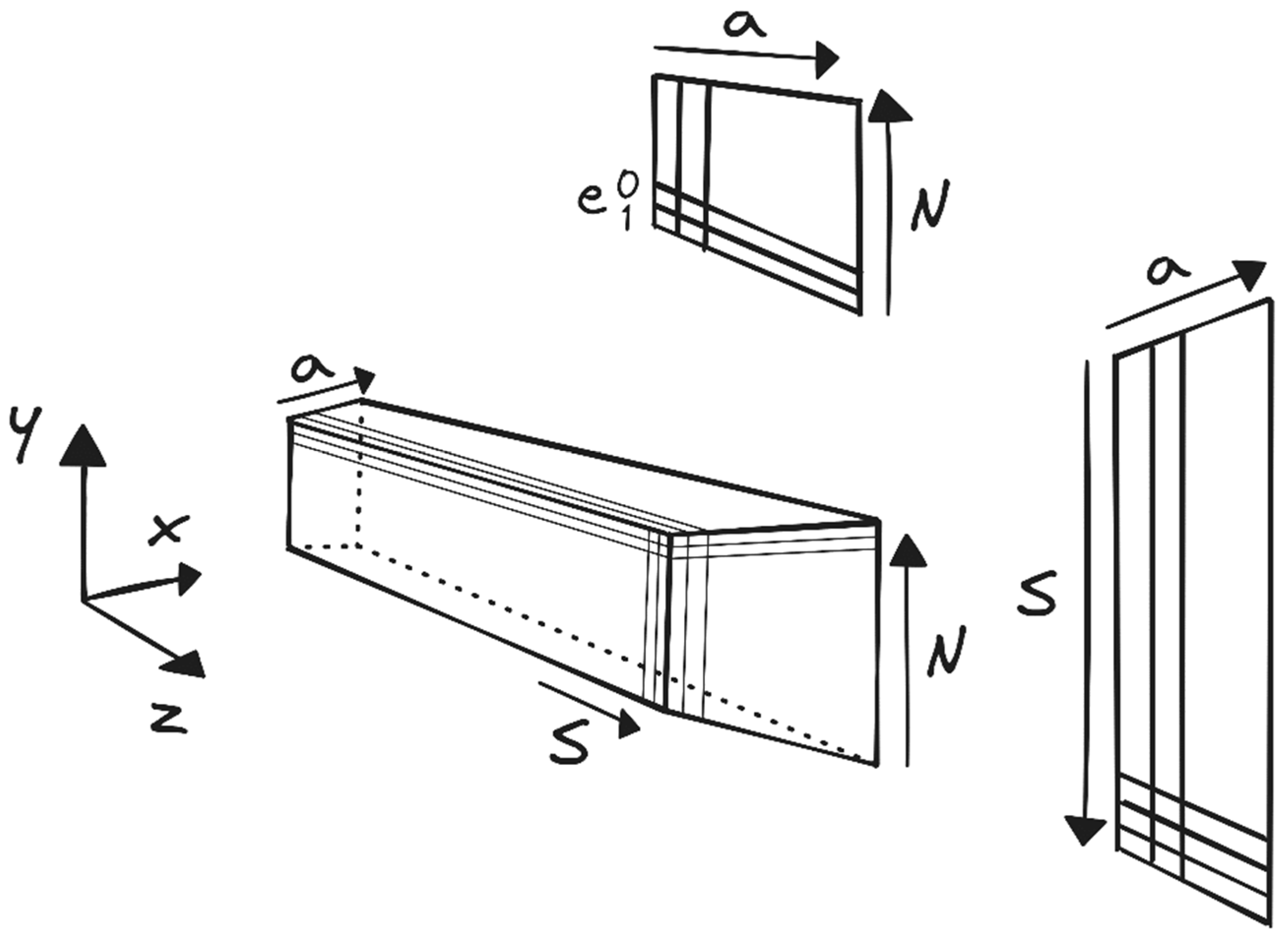
A simplified sketch of a single detector unit is provided in Figure 1. The detector’s geometrical details are represented using the following coordinate systems: $\left(x,y,z\right)$, $(2\theta ,\phi ,r)$, or the unique voxel identifier (voxel ID). This ID combines four building components: ‘a’ for the anode wire, ‘S’ for the cathode stripe, ‘N’ for the module number, and ‘e’ for the upper and lower part of each module. A detailed description of the internal detector design and of the detection process, just briefly described in the following, may be found in [9].

The neutron detection is a two-part process: first, the neutron must be captured in one of the boron layers according to Equations (1) and (2). Second, one of the reaction products, the ⁷Li or α particle, has to escape this layer.

¹⁰B + n → ⁷Li^• + α → ⁷Li + α + γ(0.48 MeV) + 2.31 MeV

(1)

¹⁰B + n → ⁷Li + α + 2.79 MeV

(2)

While the surface of each module ‘N’ is ¹⁰B-coated on the inside, the cathode stripes ‘S’, separating the upper and lower part ‘e’ of each module are ¹⁰B-coated on both sides. If a neutron is absorbed in any of those ¹⁰B layers and the reaction products escape, a charge cloud is generated signaling the voxel’s anode wire and its cathode stripe. Voxel encoding is then achieved by timely coincidence between anode and cathode signals.

In the remainder of this paper, the direction of the anode wire (a) will be referred to as the “depth” direction.

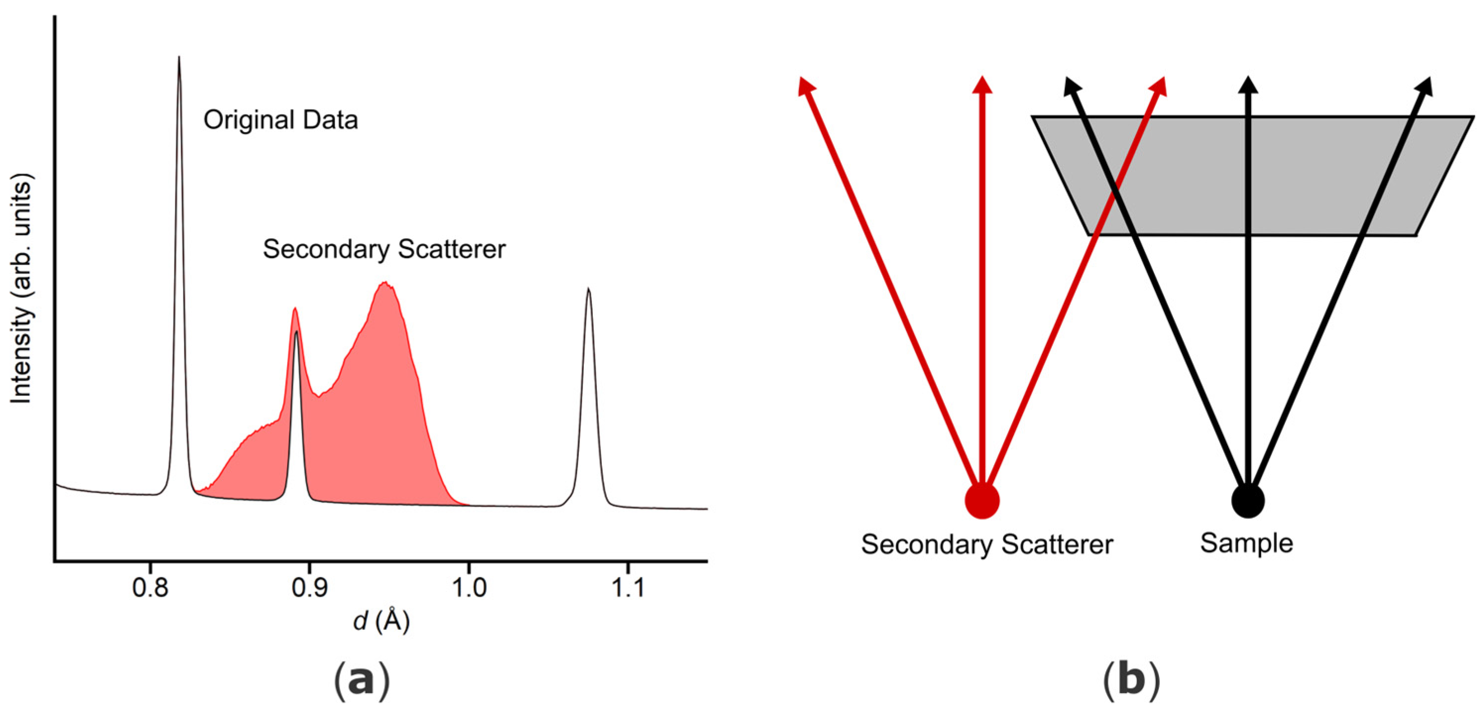
This depth is the key to a highly significant challenge in neutron-scattering experiments, namely identifying unwanted intensity contributions to the diffraction pattern from secondary scatterers. Such unwanted events arise whenever neutrons interact with unavoidable components of the experimental setup, for example the sample environment (e.g., diamond anvils in pressure cells [17]), rather than the sample itself. Conventional methods for eliminating such events often rely on additional measurements and tedious manual work by experts, but this work proposes a novel approach utilizing the additional dimension of volume detectors to aid in the identification of unwanted events.

Figure 2 provides a simplified but illustrative example of the type of unwanted events this algorithm is intended to help identify. It shows a configuration of the sample (primary scatterer, black) and secondary scatterer (red) assuming a top view of the detector in addition to the resulting diffractogram. The expected d-based diffractogram (black) can be seen alongside the red-shaded secondary scatterer intensity, which is typically broadened due to mismatched instrumental conditions (detector design concepts detailed in [9,18]).

The technique to be explored below (see Theory) has the potential to enhance the efficiency and precision of data acquisition in all future neutron-scattering experiments, not only for POWTEX but also for other volume detectors of similar design. It could easily extend to instruments such as DREAM, HEIMDAL, or MAGIC at the European Spallation Source (ESS), or even future instruments currently under development [19,20,21]. Similar to the multidimensional Rietveld method, which was originally developed for POWTEX but also applied to other TOF diffractometers within the DAPHNE4NFDI consortium [22], we anticipate a similar effort for the new technique.

2. Theory

In a plate detector, the Debye–Scherrer cone is projected onto a surface, resulting in a ring-shaped signal as depicted in Figure 3a. In a volume detector, however, the additional depth allows for the detection of multiple rings per cone, thereby providing more information about the diffracted neutrons, see Figure 3b.

As further illustrated in Figure 4, the detection of multiple Debye–Scherrer rings belonging to the same cone allows us to observe a certain intensity distribution along the depth direction.

To define an “ideal” case, the following assumptions are made:

• The time-independent conversion efficiency of each voxel is known either from an analytical description or by a reference measurement (vanadium).
• Only events from the sample are detected.
• The intensity of the first conversion layer is exactly known and attributed to a Debye–Scherrer ring.

As a consequence, Lambert–Beer’s law can be applied to calculate the intensity within deeper conversion layers:

I_p = I₀·f^p,

(3)

given p = depth, I₀ = initial intensity, f = efficiency, and I_p = intensity at depth.

3. Intermediate Results

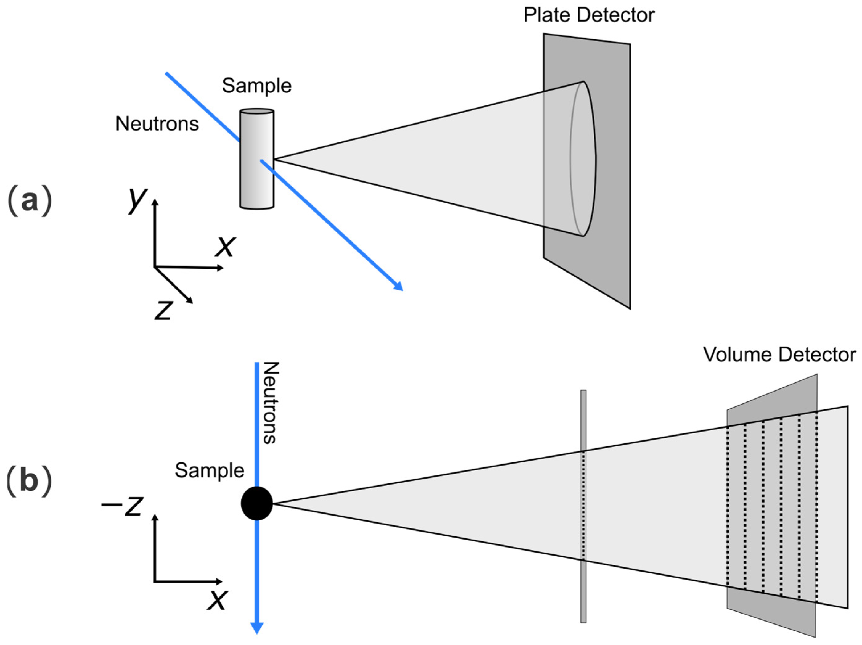
A basic intensity I vs. a plot is inadequate for representing the entire data, however, the observable distribution at a given location on the detector may differ from that observed at another location. This limitation can be readily addressed by creating a heatmap plot of the intensity I versus depth (a) and the 2θ direction (S). In this approach, the integration is performed over e and N, which both correspond to the texture angle φ. Therefore, texture is not considered in this paper.

Figure 5 illustrates two of those plots for reflections in the d-value range of 0.47 Å ± 0.05 Å for two different wavelengths (0.54 Å and 0.66 Å). Two key observations are relevant to the interpretation of the intermediate results.

First, the same reflections are observed at different detector positions for different wavelengths. Second, according to the sunray-like design of the detector stripes S as described in [18], in a monochromatic experiment (i.e., within a short time frame of the TOF experiment) one would expect a straight vertical line per reflection in Figure 5. The observation differs, however, and it is by design. To increase the point density per full-width-half-maximum, i.e., per angular detector resolution Δ2θ_Det, all stripes are linearly shifted following the depth direction from front (zero shift) to back (one full S-width shifted). This explains the jump in the detecting stripe S.

For better statistics, all the same reflections should be at the same position for different wavelengths and extend vertically without any shift. These objectives can be achieved through utilizing the diffraction-focusing method, as outlined in [23]. Bragg’s law postulates for the fulfilled diffraction conditions that the different 2θ positions for different wavelengths adhere to a specific relationship. This allows each $S(2\theta ,\lambda )$ value to be mapped to a wavelength-independent detector-stripe coordinate S′(d) for any arbitrarily chosen wavelength (${\lambda }_{\mathrm{r}}$), for example, this may be the center wavelength of the experiment.

$$2{\theta }^{\prime }=2·\arcsin \left({\displaystyle \frac{{\lambda }_{\mathrm{r}}·\sin \left(\theta \right)}{\lambda }}\right),$$

(4)

S′(a) = k_a,0 + k_a,1·2θ′ + ka,₂·(2θ′)² + k_a,3·(2θ′)³ + k_a,4(2θ′)⁴

(5)

Equation (4) employs Bragg’s law to transform the initial 2θ value into a virtual 2θ′ value with an arbitrary reference wavelength ${\lambda }_{\mathrm{r}}$. Equation (5) then takes this 2θ′ value and converts it to a discrete S′(a) value by a polynomial fit, possible due to the fixed relationship between S and 2θ for any given a. Fixing the number of coefficients in Equation (5) is largely arbitrary, and five (k_a,0 … k_a,4) was the minimum number able to adequately describe the relationship. The value of S′(a) depends on the depth a, as evidenced by the shift observed in Figure 5. The “bending” of S′ can be eliminated by calculating a S′(a) for a fixed a, thereby finally transforming S′(a = 0) into a depth- and wavelength-independent S′. Although S′ is principally continuous, it is presented and used here as a discrete value.

A visual depiction of this novel intensity representation is provided in Figure 6. This conversion is beneficial as both peak wandering and S-shifting are effectively eliminated. In the event of neutrons emanating from the sample position and oriented in alignment with the detector, a precisely vertical line with the established distribution (Figure 4) should be visible in the same position for each wavelength.

It is obvious that this method permits the simultaneous presentation and easy visual distinction of a primary and secondary scatterer from two distinct origins. Its key strength lies in the expected behavior which only events originating from the sample will follow as a function of diffraction focusing according to Bragg’s law and the intrinsic detector layout viewing on the sample. Secondary scatterers, as illustrated in Figure 2, will in contrast deviate from these expectations and hence do not align. In the I(S′, a) plot (Figure 6), these contributions manifest as smeared and distorted, in strong contrast to the straight peaks originating from the sample.

In the following, we will utilize those and similar expectations, e.g., the clear distinction based on adherence to Bragg’s law along the S′-direction as well as the expected Lambert–Beer behavior along I(S′, a), as powerful tools for removing these additional intensity contributions of an arbitrary secondary source.

By identifying and isolating the intensity contribution that deviates from the expected behavior, unwanted contributions can be effectively filtered out. As a result, the overall signal-to-noise ratio, and ultimately, the accuracy of the data can be significantly improved.

4. Experimental

Before delving into the specifics of the data processing algorithm, it is crucial to establish their foundation, namely the data themselves. This chapter will discuss both the source and the characteristics of the data used in this study.

The event neutron TOF diffraction data utilized herein originate from operating a mounting unit of the cylinder-surface detectors of POWTEX, i.e., about 2% of the voxels of the final instrument, at the neutron TOF diffractometer POWGEN at the Spallation Neutron Source (SNS) at Oak Ridge National Laboratory (ORNL, Oak Ridge, TN, USA), as indicated above. All data are stored in the Nexus format [24,25]. The analysis relies on powdered diamond as a standard sample and vanadium as usually measured for efficiency correction. The diamond measurement yielded a total of 190 million events recorded over 10 h.

It is important to note that the original dataset naturally lacked significant contributions from secondary scatterers, since originally it was not collected for this type of data treatment. To demonstrate the effectiveness of our algorithm including such unwanted events, we have incorporated (by simulation) a single additional d-reflection into the dataset. This hypothetical secondary scatterer is located at 20 cm translated along the positive z direction relative to the sample and generates a single d-reflection with d = 0.72 Å, and a FWHM of 0.005 Å. By this rather simple choice, we ensure to largely control how the developed algorithm should behave. Admittedly, in a real experimental setting, a multitude of secondary contributions may emerge, necessitating a nuanced approach to their treatment. A more detailed elaboration of this point will be provided in the Discussion Section.

For this procedure, the raw data are expectably stored in event mode containing information about the time-of-flight t the neutron has travelled and the specific voxel it was detected in $\left(x,y,z\right)$. Given the knowledge of the total flight path for every voxel since $t=0$, the time-of-flight is first converted to the wavelength. Next, the converted events are sorted and wavelength-binned with a bin width corresponding to the instrument’s natural wavelength resolution [4,26]. This temporary histogramming in terms of wavelength simplifies the following analysis.

The second step converts the voxel information into the already described detector coordinates: S (2θ direction), a (depth direction), e (upper/lower part of the module) and N (module number) as texture angle φ. This process results in a five-dimensional array representing intensity with respect to S, a, e, N, and the wavelength bin index ${\lambda }_{\mathrm{i}}$. In essence, the data preparation step transforms the raw event data into a more manageable and informative format suitable for the application of the algorithm. The resulting format is optimized for counting statistics, while retaining the ability to trace back to the original event-mode data.

Based on the created data array, several expectation-matching analyses are combined to identify unwanted events. To achieve the greatest efficiency, these algorithms should operate with portions of the array independently, allowing for a high degree of parallelization:

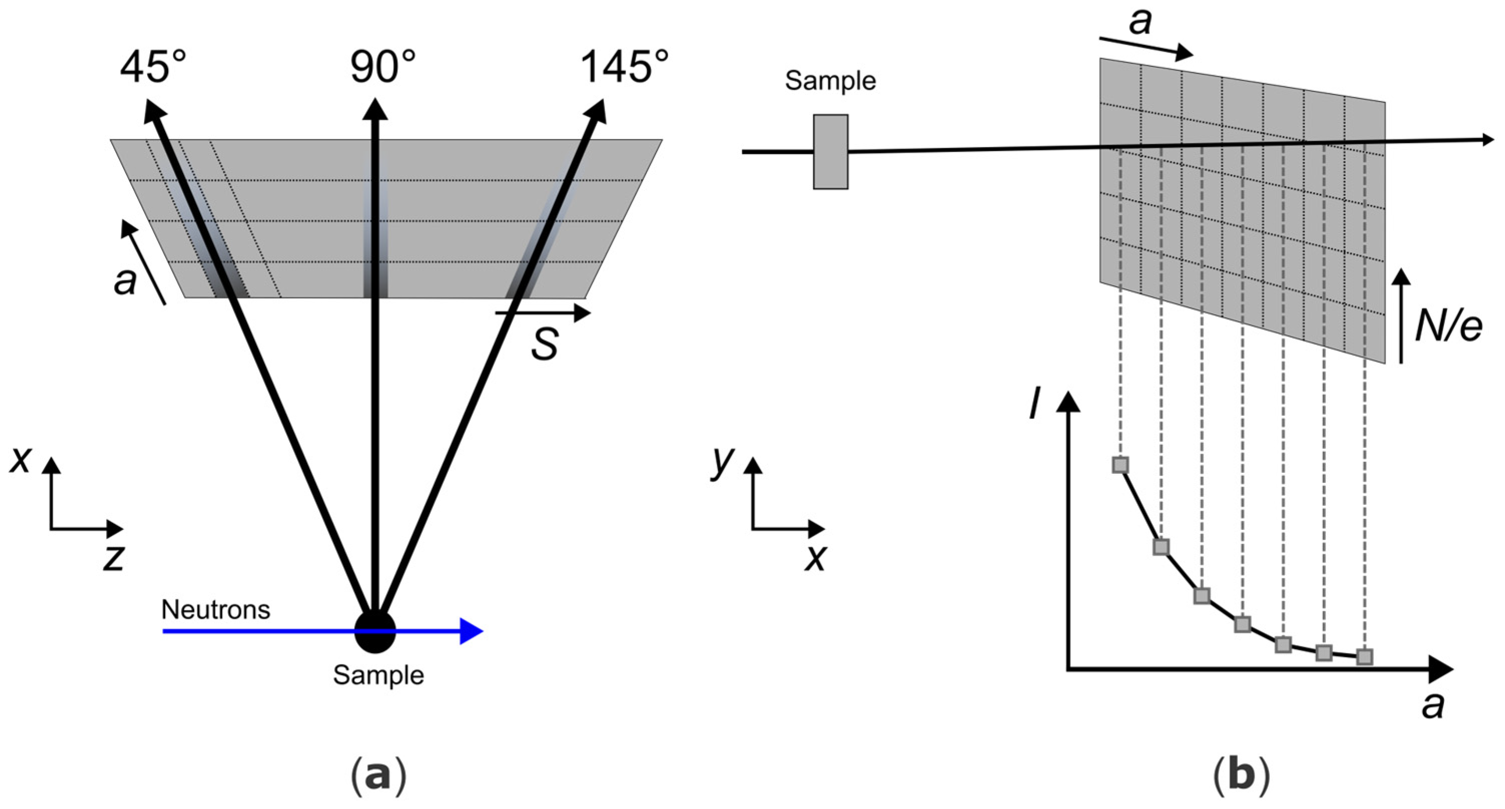
Intensity vs. Depth Plot (a): Within an individual S′ value, the intensity originating from the sample should adhere to the principles of the Lambert–Beer law, exhibiting a characteristic decrease in intensity with increasing depth (along the a direction). Erroneous data points, however, are likely to deviate from this expected exponential decay. For this to still be effective, it is necessary to know the anticipated intensity distribution, which is to be obtained through either geometric calculations or reference measurements without any secondary contributions. In this case, although the original data do not contain significant secondary contributions, the vanadium measurement is used as a reference. Furthermore, while the analysis currently focuses on isolated S′ values—due to parallelization and considering future applications—, it is worth noting that future iterations could potentially explore how intensity variations across different S′ values might also contribute to identifying outliers. For instance, the precise manner in which the intensity is shifted for the secondary scatterer provides insight into the location of the secondary scatterer.

Intensity vs. Wavelength Plot (b): As a consequence of diffraction focusing, a typical intensity-wavelength plot is not observed for a single S′ (Figure 7). Traversing the wavelength for a given S′-value is analogous to traversing one sinoidal d-reflection in the (2θ, λ)-coordinate system, quite similar to the (d, d_⟂) considerations made in [4]. This results in a rather flat, linear curve with almost constant intensity, rather than the typical distinct reflections. In contrast, erroneous events are likely to exhibit intensity variations across different wavelengths for various depths (represented by a). Such deviations present an opportunity to identify and designate them as outliers.

In essence, the two depicted representations provide valuable tools for distinguishing between valid sample data and unwanted events within the context of a specific S′ value. By identifying data points deviating from the expected behavior in both plots, the algorithm can effectively flag and remove these erroneous events, leading to a cleaner and more reliable dataset for further analysis.

It is important to note that a variety of established outlier detection methods can likely be applied in this context. Our initial exploration yielded promising results with techniques such as DBSCAN (density-based spatial clustering of applications with noise) [14]. It necessitates a relatively intricate calibration of parameters, however, and is otherwise computationally expensive by comparison. In addition to DBSCAN, we have investigated various statistical techniques to identify outliers. Since our method is under active development, we will not delve too deeply into the details and only present one of the most effective, although rather elementary, methods. The steps are as follows:

• Calculate the average over all λ for every a value (see Figure 7b);
• Divide each value for all λ and a by the expected distribution (see Figure 4 and Equation (3));
• Check for anomalies;
• Check with respect to step No. 1 if any of the values are drastically above the average (e.g., twice as large);
• Check with respect to step No. 2 if any of the values deviate drastically from the expected distribution (e.g., larger by a factor of ten);
• Calculate a new average without any of the detected anomalies;
• Define a threshold (e.g., 2.0) and flag every (λ, a) position as potentially erroneous that is above the new average times the threshold;
• Also flag around that position within a specific δ (e.g., ±3);
• Check if the erroneous sections moved along λ for different a (see Figure 7) to prevent false positives.

This method is precisely aligned with the structure of the data. However, this also implies that it is reliant on the original data exhibiting the aforementioned flat, linear intensity curve. Additionally, it depends upon the secondary scatterer data being grouped relatively close and exhibiting a notable degree of prominence. Once more sophisticated, simulated or possibly measured data become available, one may generalize the method of detection and even extend it.

It is undoubtedly feasible to implement even more sophisticated analytical techniques to examine the data structures. At the moment, however, the implementation of the outlier detection method depends on the overall algorithm. Considerations include whether the data treatment will be performed online, e.g., for fast live viewing or live decision-making, possibly enhancing in situ experiments, or offline. Accordingly, different methodologies, e.g., the application of AI-aided detection algorithms (and, hence, different target hardware platforms) will be considered, for example, field-programmable gate arrays (FPGAs), central processing units (CPUs), or graphics processing units (GPUs). Further details on this topic are given in the Results and Discussion Section.

Following the previously described identification of outliers, the algorithm then enters the correction phase. Here, we address the removal of outliers from the five-dimensional intensity array. This correction phase involves translating the information gleaned from the S′ pre-processing back into the nexus event data format, achieved by iterating through each wavelength bin and voxel within the original data. At each voxel and wavelength bin, the original intensity value is compared with the optimized, i.e., expected intensity.

There are two primary options for applying the optimized intensity to the event data:

Random Removal or Masking: Assuming that events within the same voxel and wavelength bin exhibit identical behavior, outlier removal can be achieved by randomly eliminating or masking out events until the total intensity matches the expectation value of the according trajectories. This approach leverages the inherent redundancy within the data due to the chosen wavelength resolution.

Event Weighting: Alternatively, each event can be assigned a weight based on its likelihood of being a valid data point. The sum of these weights across all events within a specific voxel and wavelength bin would then be adjusted to match the expected intensity. This method avoids data loss entirely but introduces a probabilistic element to the data. This might anyway be the case upon further data reduction. Surely, downstream algorithms need to be checked for compatibility and may be improved if the assigned weighting is considered.

It is worth noting that both options will only act on equivalent neutrons within the binning limits and that the origin or, better still, the flight direction is unknown and not part of their equivalence. Naturally, one cannot assign a specific one of these equivalent events to a known origin. Having ensured reasonable counting statistics with the help of multievent correlation, however, it is possible to assign a number of equivalent events to an expected behavior, i.e., the diffraction pattern arising from the sample, while the rest is unexpected and hence removed (or all equal events are weighted accordingly).

The data reduction algorithms usually follow after the given treatment. Herein, already at some early point, the event data are binned to yield histogram data. Hence, any previous event-to-origin correlation is lost anyway upon empty background subtraction or efficiency correction by vanadium. Purposefully, we decided to stay independent from further treatments for the moment, but as we pointed out, further algorithms may be improved when event weighting is considered.

5. Results and Discussion

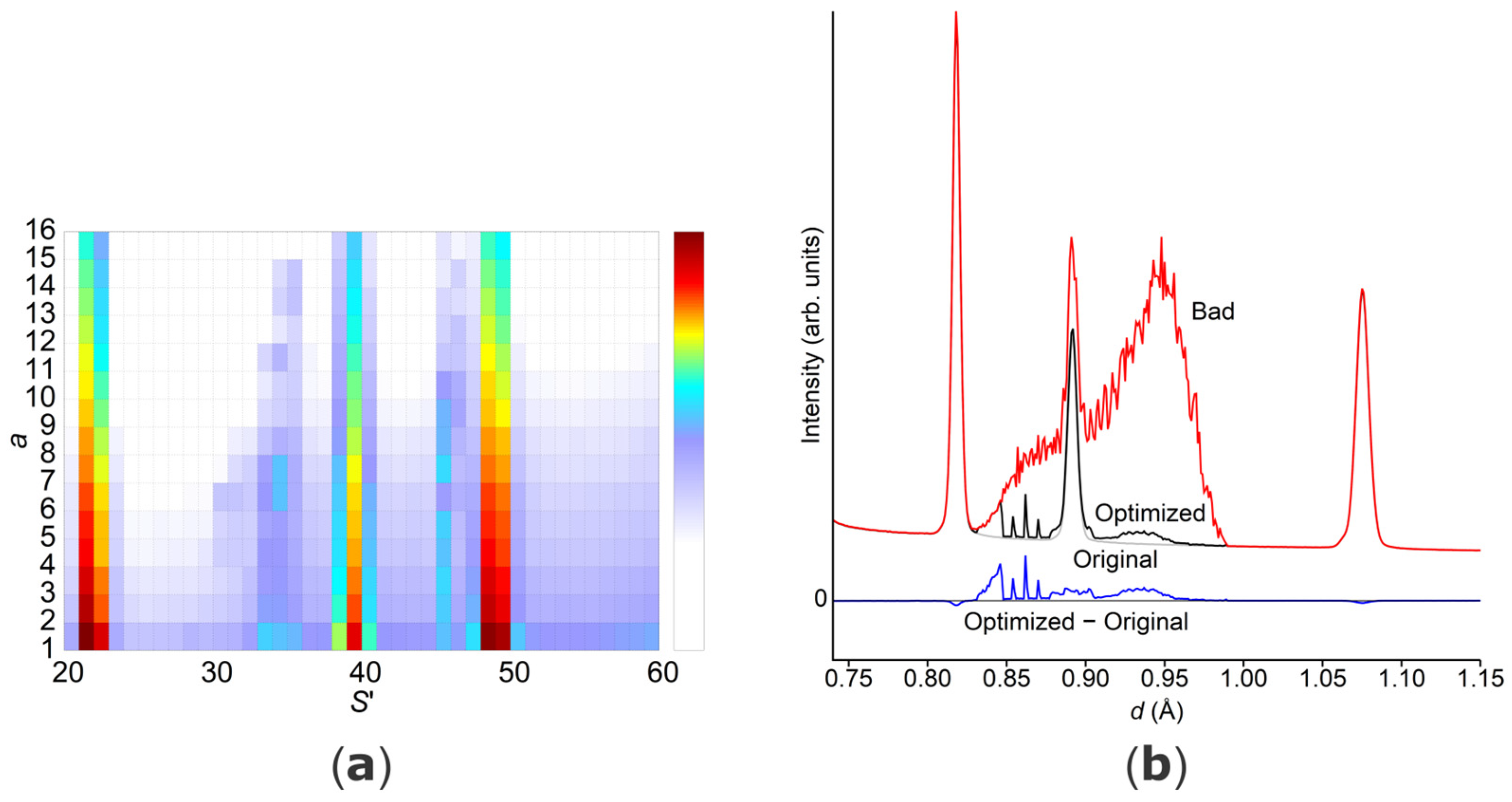
The current algorithm managed to remove 94% of the previously added, unwanted intensity while preserving over 99% of the valid data, so less than 1% of the good intensity was affected as false negatives.

Figure 8 provides a visual representation of the results, presented in two differing plots. The plot (a) on the left depicts intensity versus S′, as introduced by Figure 6. A notable reduction in secondary scatterer intensity has been achieved, and the three vertical reflections present in the original data are now easily discernible. Nonetheless, residual intensity from the secondary scatterer persists to a limited extent. The right plot (b) more effectively showcases the residual intensity. While the red curve represents the combined primary and secondary intensity, the black line corresponds to the primary intensity identified by the algorithm, whereas the blue line is the remaining secondary intensity. It is evident that the algorithm handles diffraction areas differently, with some areas being more accurately resolved than others. These findings suggest that there may be an area for potential algorithmic improvement to be explored in subsequent iterations. It is crucial, however, to acknowledge that the algorithm has demonstrated considerable success in recovering a significant portion of the original reflection, which was previously obscured entirely by the secondary intensity.

While the algorithm demonstrates effectiveness with the test data employed here, it remains under development, as said before, with ongoing improvements and potential design adaptations based on real-world cases. Looking ahead, we plan to expand our testing based on simulated data using the existing VITESS model of POWTEX [27] and a GEANT4 model similar to [2], because data control is ensured and the packages are widely accepted. This may include secondary Bragg scatterers, but also other typical contributions like air scattering or even diffuse scattering from the sample itself; either wanted or unwanted information. Of course, real experiments will lastly unveil the true performance.

A critical design decision centers around the chosen realization strategy, including whether the data optimization is performed online (during the experiment) or offline (after the experiment, i.e., with typical software like Mantid [28] or scipp [29]), and which target hardware platform (FPGAs, CPUs, or GPUs) fulfills all requirements, as mentioned already.

In an offline setting, computationally expensive but established techniques like DBSCAN or even neural networks implemented on GPUs become viable options. Conversely, online processing, often favoring FPGAs for real-time operation, necessitates careful consideration of resource limitations and efficient algorithm design. Here, factors such as the usage of floating point numbers and the necessity to avoid divisions become crucial for achieving efficient processing on hardware with limited resources. Additionally, in an online setting, the algorithm must grapple with real-time constraints. Key questions include the following: how long can the algorithm wait/how long does the algorithm need to wait for incoming data due to simple statistics, and how much time does it have to process that data before being ready for the next batch? A preliminary investigation was conducted to ascertain the necessary data volume. The same algorithm was applied to a reduced dataset comprising only 10% of the entire dataset, and the resulting accuracy was found to be only slightly affected.

The current implementation leverages an offline approach (facilitated by the absence of online experiments and ease of development) and is written in Rust [30] in a verbose manner for debugging purposes. Parallelization is a core design principle, allowing the algorithm to scale effectively with the available processing units (GPUs, CPUs, or FPGAs). This inherent scalability is expected to handle increasing data volume efficiently but warrants further investigation in the future.

We reiterate that the current analysis was performed on a very small subset of detectors, using data from a single building unit of the detector. The fully operational detector will generate significantly larger datasets. Fortunately, this might not be a hurdle and may even present opportunities for more robust statistical analysis. It is important to note, however, that some detector components exhibit slightly different geometrical details, so this necessitates potential adaptation or, ideally, generalization of the algorithm to handle these variations seamlessly.

A POWTEX scenario: A maximum performance version might envision operating on approximately 2 M voxels of the POWTEX detector, collecting approximately 10⁶ n/s, i.e., 1 MHz event rate, from the sample (very uneven spatial distribution) plus an unknown, possibly equal contribution from secondary sources (unknown distribution). This is to be scaled by the level of local detection vs. the correlation of batches, and generally, the parallelization and platform choice of the final algorithm. For example, one might integrate FPGA(s) into the optical fiber detector read-out chain, or one might also think about producer/consumer event-streaming solutions like ASAP::O [31] or Apache Kafka [32], supporting parallel and multi-platform analysis, or even a hybrid of both. ASAP::O is developed and suited for scientific instrumentation aspects and is heavily used by DESY [31]. Apache Kafka is also widespread, including, to the best of our knowledge, applications at the ESS [33] and at the Paul Scherrer Institute, Würenlingen, Switzerland, e.g., using a scintillator-based detector from CDT GmbH with a Kafka producer implemented in the common CDT Hardware library.

Next to conventional experiments, one may surely also envision to collect such high-intensity data in an in situ experiment, e.g., when following a chemical reaction or phase transition. To most efficiently use the costly neutrons, on-the-fly algorithms will be needed. The events must be visualized in real time or reduced to further analytic algorithms in order to allow for live decision-making. That is to say that experiments must be watched to decide about expected behavior, or entering a critical state where statistics must be ensured for later analysis. From conventional to sophisticated experiments, all will extensively benefit if unwanted data are removed or flagged as such, and interpretation concentrates on relevant events. For the mentioned instruments on other sources, the data rate might be even higher.

Furthermore, the established application of hardware collimators addressing a similar issue must be acknowledged. For our large detector design, conventional hardware collimators are not yet available, they are difficult to construct, and one must geometrically consider the sample environments. This also presents a timely effort when changing the sample. Additionally, there are other inherent geometrical boundary conditions that must be maintained. Last, given real-world applicability of the here-proposed method, it would support or even replace costly hardware collimators.

6. Conclusions

We have presented a novel method for the pre-processing of neutron-scattering data acquired via a time-of-flight (TOF) powder diffraction experiment using three-dimensional volume detectors, e.g., of the Jalousie type. The primary challenge addressed is the presence of secondary scatterers next to the sample, e.g., when the primary neutron beam is scattered at a sample environment. These secondary scatterers produce events that deviate from the expected type of diffraction pattern, leading to additional, undesired events in the collected data.

In the current implementation, the raw data undergo a two-step transformation to prepare them for efficient S′ analysis and outlier removal. First, the data are binned according to the wavelength of the detected neutrons, because the binning reflects the inherent resolution of the detector and simplifies subsequent analysis. After binning, the data are transformed into a representation that leverages the detector’s coordinate system. The latter utilizes existing coordinates (S: stripes, a: anode wires, e: upper/lower module part, N: module) and introduces a new virtual 2θ′ value (S′) derived through diffraction focusing. This allows for independent analysis of each S′ value to identify, flag, and if desired, remove erroneous data not corresponding to the expected intensity distribution regarding wavelength, stripes S′, and depth a.

Once outliers have been identified and flagged, they can be removed from the intermediate data representation, and subsequently removed from the reduced raw event data. The correction phase involves comparing the original with the optimized intensity (after outlier removal) for each voxel and wavelength bin within the raw data.

The results of the algorithm operating on the first available test data demonstrate its significant effectiveness, successfully removing unwanted intensity while preserving a high percentage of valid data. Based on these promising results, the next step will be to set the course for future actions and implementations, e.g., with an application at the POWTEX instrument.