Analysis of Traffic Injury Crash Proportions Using Geographically Weighted Beta Regression

Abstract

The classical linear regression model allows for a continuous quantitative variable to be modeled simply from other variables. However, this model assumes independence between observations, which, if ignored, can lead to methodological issues. Additionally, not all data follow a normal distribution, prompting the need for alternative modeling methods. In this context, geographically weighted beta regression (GWBR) incorporates spatial dependence into the modeling process and analyzes rates or proportions using the beta distribution. In this study, GWBR was applied to the traffic injury (fatal and non-fatal) crash proportions in Fortaleza, Ceará, Brazil, from 2009 to 2011. The results demonstrated that the local approach using the beta distribution is a viable model for explaining the traffic injury crash proportions, due to its flexibility in handling both symmetric and skewed distributions. Therefore, when analyzing rates or proportions, the use of the GWBR model is recommended.

1. Introduction

In 1997, the Swedish parliament initiated a debate on the Vision Zero program, which aims for zero serious and fatal traffic accidents [1]. To achieve this goal, the program acknowledges that several factors contribute to safe mobility, including road geometry, set maximum speeds, and the technology used in traffic studies and control policies [2]. Accidents can still occur, however, serious and fatal crashes would be less observed. Ref. [3] adopted Resolution A/RES/74/299 on improving global road safety, proclaiming the Decade of Action for Road Safety 2021–2030. This initiative sets the ambitious target of preventing at least 50% of road traffic deaths and injuries by 2030.

Following [4], in 2019, deaths from road accidents ranked 12th among the causes of total deaths worldwide, ahead of causes such as tuberculosis (13th), HIV (14th), and homicides (17th). When focusing on the younger population, aged between 5 and 49 years, for the same year, there is a significant shift in this ranking, causing deaths from traffic accidents to now be in third place, behind only cardiovascular diseases and neoplasms, such as cancer.

Examining the occurrences in some countries over recent years using data from [5], and adjusting occurrences according to population size to reflect the number of deaths per 100,000 inhabitants, one can observe the case of Thailand, which shows considerable growth in the rate, reaching almost 30 deaths per 100,000 inhabitants in 2019. Another country that had very high rates but has managed to reduce them is Brazil; in 2019, it still had a high rate of approximately 15 deaths per 100,000 inhabitants, a decrease from the beginning of the series in 2010, when there were 21 deaths per 100,000 inhabitants on the roads. To the detriment of these countries, Sweden serves as an exemplary model in this fight, managing to maintain a rate of close to 3 deaths per 100,000 inhabitants until 2018. It is worth mentioning that Sweden is the pioneer of Vision Zero, which began in 1994 [1].

Therefore, techniques to establish the relationship between two or more variables in the pursuit of modeling traffic crashes are widely studied. Among these techniques, classical linear regression is one of the most widespread statistical methodologies, allowing a continuous quantitative variable to be modeled from other variables. This method is widely used for its simplicity and applicability in several areas such as research and marketing. However, classical linear regression has some assumptions that are often overlooked, leading to methodological issues and potentially erroneous conclusions about the study. Assumptions such as the independence between observations and the Gaussian distribution of errors (or the response variable), if not properly assessed, can yield inaccurate results [6]. Thus, several other methods have been studied and developed to adapt to situations that do not meet the assumptions of classical linear regression, such as generalized linear models and spatial models.

In the case of discrete data, such as the number of traffic crashes, classical linear regression has some limitations, as indicated by [7,8,9]. According to [7], the use of a classical linear regression for discrete data may include the presence of unwanted statistical properties, such as the possibility of a negative crash count and the lack of adjustment to the distribution itself, due to the asymmetry common to the aforementioned data. In these cases, the use of Poisson or negative binomial regression models is more recommended.

When the interest lies in modeling the traffic injury crash proportions, a barrier to using a regression model for discrete data is that the value is continuous and restricted to the interval [0, 1]. It is also not appropriate to use classical linear regression, even if the data are continuous, because the data may exhibit right-skewness since the proportion of traffic injury crashes is generally low relative to the number of crashes. For situations like this [10], the beta regression model is considered, which assumes that the response variable follows a beta distribution. This distribution is supported by the continuous unit interval (0, 1) and offers the flexibility to model both symmetric and skewed data.

In order to incorporate the spatial factor into the study of traffic crashes, ref. [11] suggests the use of models that consider spatial dependence, given the influence between events that occur closer to each other. This dependency structure was also verified by [12,13], among others. Combining the concepts of beta regression and geographically weighted regression, defined by [14,15], the authors developed the geographically weighted beta regression (GWNBR). This approach seeks to model rates and proportions in a spatial context.

Thus, this work aims to apply the GWBR model developed by [15] to traffic crashes that occurred in the city of Fortaleza, Ceará, between 2009 and 2011, considering the proportion of traffic injury (fatal and non-fatal) crashes.

2. Background

In reviewing the literature on traditional approaches to road and highway planning, there is a clear lack of explicit consideration for traffic safety issues and concerns [16]. To show this, a scheme was proposed by [17] to make the concept of security in the traffic system more apparent. In this new scheme, safety is an integral part of constructing the transportation network, being considered at each stage, from the addition of new accident information to the incorporation of new traffic volumes into the network. In addition, within the planning stage, actions for future security are also evaluated, thus adopting a proactive approach to this aspect.

As the vision of traffic planning has evolved, tools are needed to support this advancement, stimulating the search for more advanced techniques to model traffic crashes in a more objective/precise way, thus generalizing problems to avoid such incidents. For this, several studies aim to model such occurrences, with several different approaches, as shown in [11,18,19,20,21].

Some characteristics to consider when modeling traffic crashes and aiming to proactively address such events include exposure to risk (traffic volume, mileage), the probability of involvement in an accident based on predefined characteristics, and the severity of the crash [16]. The latter is extremely important for the work developed here, as the main focus is on the Vision Zero strategy, which aims to eliminate serious and fatal crashes [1].

To perform the modeling, one should consider a spatial aggregation of occurrences by area units, such as census tracts, neighborhoods, or, most commonly in the modeling of traffic crashes, the traffic analysis zone (TAZ), as used by [11,12,19,22,23,24].

TAZs are geographic units constructed based on clusters according to the sociodemographic characteristics of the locality [25]. The first systematic algorithm aimed at defining TAZ was proposed by [26], optimizing an objective function for partitions of a locality based on some observed variables. Since then, this method of separation has been one of the most utilized for transportation planning.

The frequency of crashes can then be estimated for each TAZ according to the associated attributes, such as the following:

• Road characteristics: Volume of intersections [27], roads with different speed limits [22,28], roads with different classifications [19,27,29], intersections, and roundabouts [19];
• Traffic pattern in terms of the volume and speed of the road [19,29];
• Origin and distribution of the route [28];
• Weather conditions [30];
• Land use [22,29];
• Socioeconomic factors: population density [27,31], age [19,29,30], family income [22,27,32] and employment [19,27,29].

Some proposals have been made for the modeling of traffic crashes, where the spatial factor is omitted, such as the generalized linear model with the negative binomial distribution [19,28,30,31] and the Bayesian lognormal Poisson model [22,32]. For models that consider spatial dependence, the literature contemplates a Bayesian approach [19,27,30], as well as frequentist models, such as econometric spatial models [19], geographically weighted Poisson regression (GWPR) [29,33], and geographically weighted negative binomial regression (GWNBR) [11].

It is seen that the factors for the aforementioned models include characteristics of the vehicle’s driver and the road, thus confirming the need for a joint approach of these factors for the construction of the safest traffic model, as indicated by [17,34]. Given this, several approaches are taken, and one of them is Zero Vision.

For this modeling, some studies do not delve into the inferential part but explore the relationship of fatal crashes with the place of occurrence, as in [35,36] that use kernel density estimates. Among the inferential statistical models, the use of logistic regressions is more common, either without incorporating the spatial factor [37,38,39] or by including locality in the model, as presented in [40], through conditional logistic regression stratified by locality.

Some studies use the count of fatal crashes as a dependent variable, such as [30], which considers modeling using the negative binomial distribution and a Bayesian approach, and [24], which considers econometric spatial models. In this context, some methodological flaws in the aforementioned works are noted. One issue is the probable spatial dependence of the occurrences, which violates the fundamental assumption of the independence of observations. Another flaw arises from using the count of traffic injury crashes since this count is naturally influenced by the number of cars in the locality and not solely by the severity of the crash in a given place, which is the factor this study seeks to understand.

Because of this, the analysis developed here seeks a better adaptation of the data to the real distribution, incorporating the spatial dependence of the occurrences, without disregarding the numerous advances, such as the predetermination of fundamental factors for the modeling of traffic injury crashes.

Geographically Weighted Beta Regression (GWBR)

The beta distribution has density given by the following:

$$f\left(y\right|\alpha ,\beta )=\frac{\mathrm{\Gamma }(\alpha +\beta )}{\mathrm{\Gamma }\left(\alpha \right)\mathrm{\Gamma }\left(\beta \right)}{y}^{\alpha -1}{(1-y)}^{\beta -1}$$

(1)

where $0<y<1$, $a>0$, $b>0$, and $\mathrm{\Gamma }(.)$ is the gamma function. The $\alpha$ and $\beta$ parameters define the various shapes of the beta distribution.

Since the intention is to define a regression model, it is more interesting to reparameterize the beta distribution as a function of its mean ($\mu$) and consider a parameter for the precision ($\varphi$) [10].

Ref. [10] developed a model suitable for situations in which the behavior of the response variable can be modeled as a function of a set of explanatory variables, as in a traditional regression, taking into account the response variable following the beta distribution, which restricts the analysis to the continuous interval (0, 1) and which has great flexibility for modeling.

Ref. [10] proposed a reparameterization, considering $\mu =\alpha /(\alpha +\beta )$ and $\varphi =\alpha +\beta$, so that

$$\mathrm{E}\left(y\right)=\mu \mathrm{and}\mathrm{Var}\left(y\right)=\frac{V\left(\mu \right)}{1+\varphi }=\frac{\mu (1-\mu )}{1+\varphi }$$

(2)

The reparameterization of the beta distribution as a function of the mean $\mu$ and the precision parameter $\varphi$ is [10] is as follows:

$$f\left(y\right|\mu ,\varphi )=\frac{\mathrm{\Gamma }\left(\varphi \right)}{\mathrm{\Gamma }\left(\mu \varphi \right)\mathrm{\Gamma }\left(\right(1-\mu \left)\varphi \right)}{y}^{\mu \varphi -1}{(1-y)}^{(1-\mu )\varphi -1}$$

(3)

where $0<\mu <1$ and $\varphi >0$.

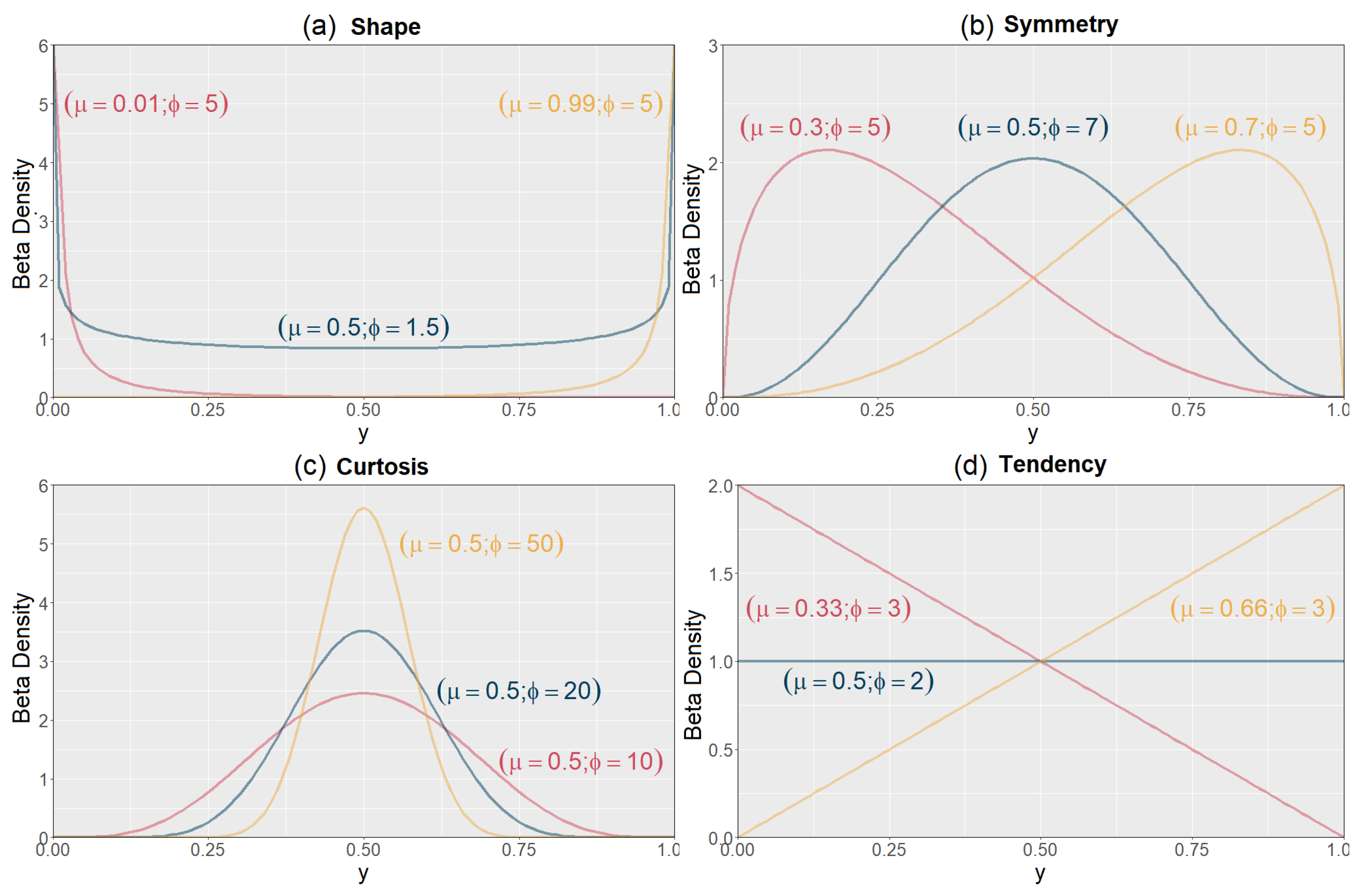
Note that the $\mu$ and $\varphi$ parameters (such as the original $\alpha$ and $\beta$) define the various shapes of the beta distribution (Figure 1). It is possible to obtain an inverted J, U, or J-shaped distribution (a), with different symmetries (b) or heavy tails of the distribution (c), or even fit a linear behavior (d).

For the geographically weighted beta regression model, developed by [15], it can be assumed that the average of the response variable at location i can be modeled as follows:

$$g\left({\mu }_i\right)={\eta }_i=\sum _k^p{\beta }_k(u_i,v_i)x_{ik}i=1,\dots ,n$$

(4)

where $g(.)$ is a link function that associates the interval $(0,1)$ to $\mathbb{R}$, $(u_i,v_i)$ represents the geographical coordinates of the i-th observation, $i=1,...,n$, ${\beta }_k(u_i,v_i)$ is the parameter for the k-th explanatory variable as a function of the location of the i-th observation, and $x_{ik}$ is the value of the k-th explanatory variable for location i.

Some choices for the link function $g(.)$, according to [10], are the logit $g\left(\mu \right)=log\{\mu /(1-\mu \left)\right\}$; the probit $g\left(\mu \right)={\Phi }^{-1}\left(\mu \right)$, where $\Phi (.)$ is the cumulative distribution function of a standard normal random variable; the log–log $g\left(\mu \right)=-log\{-log(\mu \left)\right\}$; and the complementary log–log $g\left(\mu \right)=log\{-log(1-\mu \left)\right\}$.

As in the beta regression model, there is no closed way to estimate the parameters ${\beta }_k$ and $\varphi$, requiring the use of numerical maximization methods of the logarithm of the local likelihood function. For these optimizations, the authors of [15] recommend using adaptations of the initial values of the beta regression as a starting point for the algorithm, considering a spatial matrix of weights ${\mathit{W}}_i$, based on the distances between the estimated location and all observed points.

The initial values of the parameter vector, ${\beta }_{0i}$, are estimated using the classical geographically weighted regression (GWR) [14], considering ${\check{y}}_i=g\left(y_i\right)$, as follows:

$${\mathit{\beta }}_{0i}={\left({\mathit{X}}^{\top }{\mathit{W}}_{\mathit{i}}\mathit{X}\right)}^{-1}{\mathit{X}}^{\top }{\mathit{W}}_{\mathit{i}}\check{\mathit{y}}$$

(5)

where ${\mathit{W}}_{\mathit{i}}$ is a diagonal matrix with the weights $w_{ij}$; it can be defined according to [14] using the biquadratic adaptive kernel for an adaptive bandwidth of the following form:

$$w_{ij}=\left\{\begin{array}{cc}{\left[1-{\left(d_{ij}/b\right)}^2\right]}^2,\hfill & \mathrm{if}j\mathrm{is}\mathrm{one}\mathrm{of}\mathrm{the}n-\mathrm{th}\mathrm{nearest}\mathrm{neighbors}\mathrm{of}i.\hfill \\ 0,\hfill & \mathrm{otherwise}\hfill \end{array}\right.$$

(6)

where $d_{ij}$ is the distance between i and j and b is the bandwidth, or according to a fixed bandwidth using the Gaussian kernel function [14], as follows:

$$w_{ij}=exp\left\{-\frac{1}{2}{\left(\frac{d_{ij}}{b}\right)}^2\right\}$$

(7)

In both cases, the optimal value for the bandwidth can be found by minimizing the cross-validation (CV) or AICc, as shown in [41].

For the initial value of the precision parameter for the location $(u_i,v_i)$, the following can be used:

$${\varphi }_{0i}=\frac{1}{n}\sum _{j=1}^n\frac{{\check{\mu }}_{0j}(1-{\check{\mu }}_{0j})}{{\check{\sigma }}_{0j}^2}-1$$

(8)

where ${\check{\mu }}_{ij}=g^{-1}\left({\mathit{x}}_j^{\top }{\left({\mathit{X}}^{\top }{\mathit{W}}_{\mathit{i}}\mathit{X}\right)}^{-1}{\mathit{X}}^{\top }{\mathit{W}}_{\mathit{i}}\check{\mathit{y}}\right)$, being ${\mathit{x}}_j$ a j-th row of the matrix $\mathit{X}$ and ${\check{\sigma }}_{0j}^2=\frac{{\check{\mathit{e}}}^{\top }\check{\mathit{e}}}{(n-p_e)g^{\prime }{\left({\check{\mu }}_{0j}\right)}^2}$, where $\check{\mathit{e}}$ is the residual of the classical GWR considering $\check{\mathit{y}}$ and $p_e=2{\nu }_1-{\nu }_2$, the effective number of parameters of the classical GWR model, with ${\nu }_1$ being the trace of the matrix $\mathit{S}$ and ${\nu }_2$ being the trace of ${\mathit{S}}^{\top }\mathit{S}$ [14].

More details about the GWBR model can be viewed in [15].

3. Application

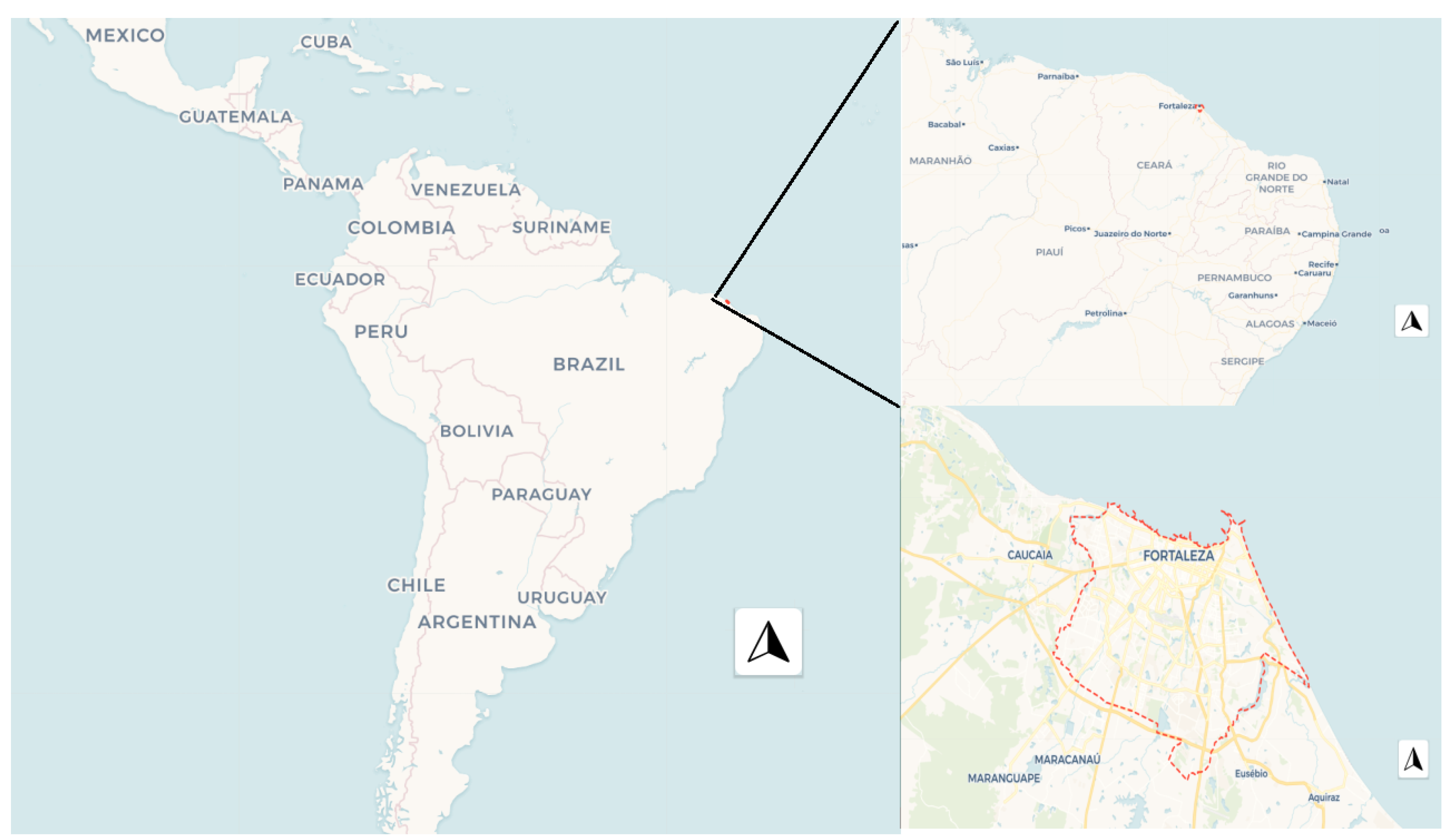
This section aims to demonstrate the fit of beta regression and GWBR to data from the city of Fortaleza, Brazil (Figure 2), which contains 126 TAZs, with socioeconomic information and land use data obtained from the 2010 Census. Along with this, the road accident data system of Fortaleza (SIAT/FOR) provided variables of the network infrastructure, including the locations of traffic lights, speed cameras, and details on crashes that occurred from 2009 to 2011, including the geolocation of these accidents and information about the presence of victims in these incidents. The database is the same one used by [11], but the analysis now focuses on the proportions of traffic injury (fatal and non-fatal) crashes, rather than the frequency of traffic injury crashes.

3.1. Data Preparation

The variables in the database, divided into six different categories, along with some of their descriptive statistics, are presented in

Table 1. Descriptive statistics of the variables.

Category	Variable	Description	Avg	Sum	Min	Max	SD
General	ID	TAZ Code	-	-	-	-	-
	X	Longitude coordinate (UTM, Datum WGS 84)	-	-	-	-	-
	Y	Latitude coordinate (UTM, Datum WGS 84)	-	-	-	-	-
	AREA_KM	TAZ area in km${\hspace{0.25em}}^2$	$2.41$	$303.14$	$0.14$	$13.48$	$2.58$
Crashes	ACT	#Crashes	$431.66$	$54,389$	6	2981	$450.92$
	ACVF	Injury (fatal) crashes	$5.54$	698	0	24	5
	ACV	Injury (fatal and non-fatal) crashes	$153.40$	$19,328$	4	829	$119.94$
Exposure Variable	EXT_TOT	Total TAZ road length (km)	$33.26$	$4190.18$	$2.63$	$192.07$	$26.89$
	POP_TOT	Total TAZ population	$19,213.86$	$2,420,946$	1183	$115,279$	$16,846.7$
Network Characteristics	DEN_I_SEM	#Signalized intersections per km	$0.3$	$37.6$	0	$1.94$	$0.35$
	DEN_I_NSEM	#Non-signalized intersections per km	$6.11$	$769.4$	$3.58$	$9.71$	$1.18$
	D_EQUI_FE	#Speed cameras per km	$0.07$	$8.41$	0	$0.39$	$0.07$
Socioeconomic Features	P_0_17	Proportion of Inhabitants between 0 and 17 years old	$0.26$	-	$0.16$	$0.37$	$0.05$
	P_18_64	Proportion of Inhabitants between 18 and 64 years old	$0.66$	-	$0.59$	$0.72$	$0.03$
	P_M64	Proportion of Inhabitants aged 65 years old or over	$0.07$	-	$0.03$	$0.14$	$0.03$
	P_D_A3SM	Proportion of households with incomes up to 3 minimum wages *	$0.58$	-	$0.08$	$0.92$	$0.22$
	P_D_M3SM	Proportion of households with an income of over 3 minimum wages *	$0.42$	-	$0.08$	$0.92$	$0.22$
Land use	URES_A	Residential land use (m${\hspace{0.25em}}^2$) per TAZ area (km${\hspace{0.25em}}^2$) (×1000)	$0.24$	$30.18$	$0.00$	$1.55$	$0.24$
	UCOPS_A	Commercial land use (m${\hspace{0.25em}}^2$) per TAZ area (km${\hspace{0.25em}}^2$) (×1000)	$0.09$	$11.68$	$0.00$	$0.74$	$0.1$

* Minimum wage of approximately USD 300.00.

.

Two dependent variables will be studied: ${\mathrm{AC}}_{\mathrm{P}}=\frac{\mathrm{ACV}}{\mathrm{ACT}}$ and ${\mathrm{ACF}}_{\mathrm{P}}=\frac{\mathrm{ACVF}}{\mathrm{ACT}}$. The purpose of using these two dependent variables is to show the potential of the GWBR technique in modeling proportions, symmetric or skewed, in contrast with the use of classical GWR, which assumes that the data follow a symmetric Gaussian distribution. Note that in Figure 3, the distribution of the variable ${\mathrm{AC}}_{\mathrm{P}}$ shows some symmetry while the variable ${\mathrm{ACF}}_{\mathrm{P}}$ is highly skewed to the right. In addition, by analyzing the goodness-of-fit of the normal and beta distributions to the data for the variable ${\mathrm{AC}}_{\mathrm{P}}$, it is clear from the Kolmogorov–Smirnov test [42] that the two proposed distributions fit the data with higher evidence for the beta distribution. For the variable ${\mathrm{ACF}}_{\mathrm{P}}$, it is clear that only the beta distribution fits the data.

The preliminary selection of the variables was based on the analysis of the correlation matrix involving each variable and the two dependent variables. After checking the correlations and avoiding possible multicollinearity problems,

Table 2. Correlation matrix with the variables to be used in the models.

	${\mathbf{AC}}_{\mathbf{P}}$	P_D_A3SM	DEN_I_SEM	D_EQUI_FE
${\mathrm{AC}}_{\mathrm{P}}$	1	$0.7956$	$-0.5806$	$-0.3185$
P_D_A3SM	$0.7956$	1	$-0.6307$	$-0.3297$
DEN_I_SEM	$-0.5806$	$-0.6307$	1	$0.4028$
D_EQUI_FE	$-0.3185$	$-0.3297$	$0.4028$	1

shows the candidate variables to explain the traffic injury (fatal and non-fatal) crash proportions (${\mathrm{AC}}_{\mathrm{P}}$).

It can be seen that the factor most strongly associated with traffic injury crashes is the proportion of households with incomes of up to three minimum wages (P_D_A3SM) with $\rho =0.7956$ (p-value < 0.0001), indicating that in locations with lower family incomes, more traffic injury crashes occur.

The greatest negative correlation ($\rho =-0.58$ (p-value < 0.0001)) in relation to the response variable occurs with the #Signalized intersections per km (DEN_I_SEM) variable. Thus, the greater the number of intersections with traffic lights, the lower the traffic injury crashes. The other variable chosen is the #Speed cameras per km, which has a correlation of $\rho =-0.32$ (p-value = 0.0003) with the response variable.

Table 3. Correlation matrix with the variables to be used in the models.

	${\mathbf{ACF}}_{\mathbf{P}}$	P_0_17	DEN_I_SEM	AREA_KM
${\mathrm{ACF}}_{\mathrm{P}}$	1	$0.5483$	$-0.4503$	$0.3746$
P_0_17	$0.5483$	1	$-0.6866$	$0.3862$
DEN_I_SEM	$-0.4503$	$-0.6866$	1	$-0.3246$
AREA_KM	$0.3746$	$0.3862$	$-0.3246$	1

shows the candidate variables to explain the traffic injury (fatal) crash proportions (${\mathrm{ACF}}_{\mathrm{P}}$).

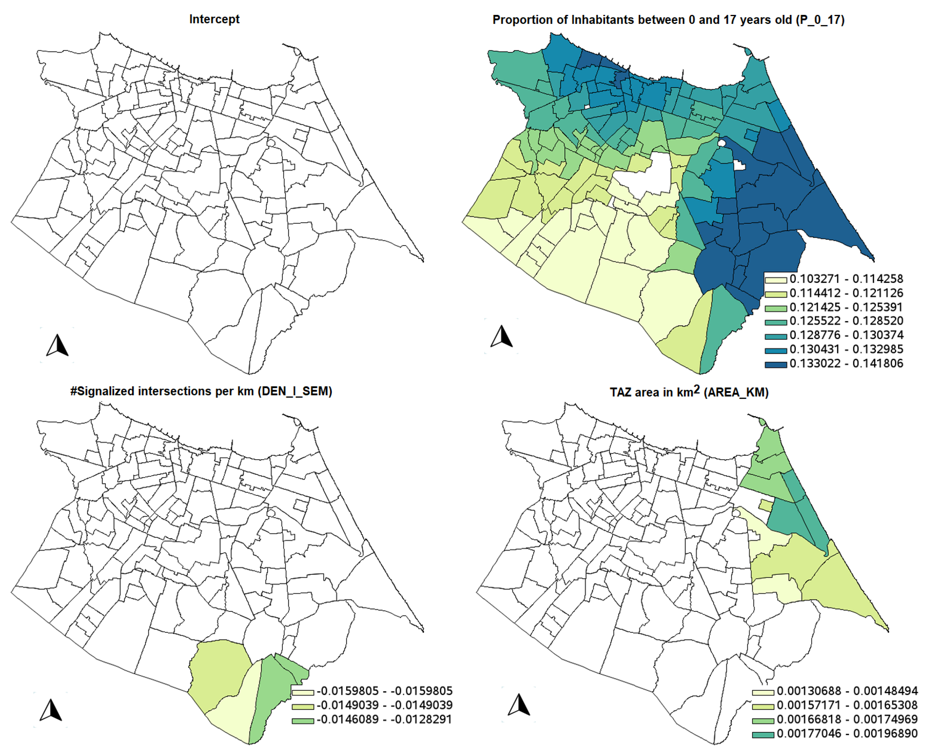
It can be seen now that the factor most associated with traffic injury (fatal) crashes is the proportion of inhabitants between 0 and 17 years old (P_0_17), with a correlation of $\rho =-0.6866$ (p-value < 0.0001) indicating that in locations with a higher proportion of young people, more fatal traffic injury crashes occur. The variable #Signalized intersections per km (DEN_I_SEM) continues to explain the fatal traffic injury crash proportions ($\rho =-0.4503$ (p-value < 0.0001)) and the TAZ area (AREA_KM) variable was incorporated into the analysis, showing a positive correlation of 37% (p-value < 0.0001).

All analyses were performed using SAS 9.4 and R software, and the GWBR model was estimated using the ‘gwbr’ package developed by the authors.

3.2. Analysis of the Variable Traffic Injury (Fatal and Non-Fatal) Crash Proportions (${\mathrm{AC}}_{\mathrm{P}}$)

The estimates of the classical linear regression model are quite different from those obtained by the beta regression with the logit link function (

Table 4. Results of global models (dependent variable: ${\mathrm{AC}}_{\mathrm{P}}$).

Variable	Classical Linear Regression			Beta Regression (Logit)
	Estimate	t	p -Value	Estimate	t	p -Value
Intercept	$0.1809$	$5.45$	<$\hspace{0.25em}0.0001$	$-1.3532$	$-9.69$	<$0.0001$
P_D_A3SM	$0.4487$	$10.13$	<$\hspace{0.25em}0.0001$	$1.9165$	$10.29$	<$\hspace{0.25em}0.0001$
DEN_I_SEM	$-0.0457$	$-1.65$	$0.1022$	$-0.2184$	$-1.85$	$0.0662$
D_EQUI_FE	$-0.0682$	$-0.62$	$0.5334$	$-0.3224$	$-0.71$	$0.4788$
$\varphi$	-	-	-	$37.4164$	$8.04$	<$\hspace{0.25em}0.0001$
Adj $R^2$ *	$0.6357$			$0.6535$
AICc	$-267.7472$			$-276.5724$
log-likelihood	$138.0389$			$143.5261$

* Pseudo Adj R² for beta regression.

); however, the interpretation of these parameters is also performed differently.

For classical linear regression, an increase of 1% in the proportion of households with incomes up to three minimum wages (P_D_A3SM) results in an average increase of 0.45% in the traffic injury crash proportions. An increase of one unit in the #Signalized intersections per km (DEN_I_SEM) results in an average decrease of 4.57% in the traffic injury crash proportions. Finally, #Speed cameras per km (D_EQUI_FE) is not significant for the model.

In the beta regression, where interpretation is based on the odds ratio, an increase of 1% in the proportion of households with incomes up to three minimum wages (P_D_A3SM) increases the likelihood of traffic injury crashes by a factor of 6.8 times ($e^{1.9165}$). Increasing the #Signalized intersections per km (DEN_I_SEM) by one unit decreases the chance of traffic injury crashes by 19.6% in the chance of occurrence of traffic injury crashes. The variable #Speed cameras per km (D_EQUI_FE) is also not significant.

Regarding the goodness-of-fit of the models, beta regression shows better metrics, considering the values of the adjusted $R^2$, AICc, and log-likelihood, even though they are not so different (but this is because the data show some symmetry).

Now, the idea is to fit local models (GWR and GWBR) to the data. The first step is to find the best bandwidth.

Table 5. The best bandwidths found for GWR and GWBR models.

Metric	GWR				GWBR
	Fixed		Adaptive		Fixed		Adaptive
	AICc	CV	AICc	CV	AICc	CV	AICc	CV
Bandwidth	$610.29$	$2125.06$	7	31	$11873.64$	$5103.32$	125	118
Adj $R^2$	$0.88$	$0.81$	$0.88$	$0.81$	$0.67$	$0.73$	$0.64$	$0.67$
ENP	$120.40$	$42.63$	$118.02$	$42.97$	$4.82$	$8.96$	$3.98$	$4.10$
Log-likelihood	$402.40$	$202.11$	$378.71$	$204.78$	$147.91$	$164.26$	$141.48$	$140.54$
AICc	$5781.78$	$-273.82$	$3506.48$	$-277.56$	$-284.27$	$-301.71$	$-278.97$	$-278.68$

Red shows the best value for the metric.

shows the bandwidth metric selection for GWR and GWBR models.

Note that for the GWR model, the effective number of parameters (ENP) is not as large when a CV is minimized (this is an important issue to avoid overfitting), and because the other metrics are quite close, and the AICc is smaller in an adaptive bandwidth, an adaptive bandwidth of 31 neighbors was selected. For the GWBR model, better metrics are found for a fixed bandwidth when a CV is minimized, and because of that, a fixed bandwidth of 5.1 km (or 5103.32 m) is selected.

Table 6. Descriptive statistics of the GWR model (dependent variable: ${\mathrm{AC}}_{\mathrm{P}}$).

Variables	Coefficients
	Min	Q1	Median	Mean	Q3	Max
Intercept	$0.0813$	$0.1787$	$0.2213$	$0.2455$	$0.2730$	$0.5628$
P_D_A3SM	$-0.1066$	$0.1997$	$0.3128$	$0.3171$	$0.4661$	$0.6651$
DEN_I_SEM	$-0.3807$	$-0.1347$	$-0.0738$	$-0.0945$	$-0.0257$	$0.0252$
D_EQUI_FE	$-1.1821$	$-0.2116$	$-0.0899$	$-0.0755$	$0.0835$	$0.6184$
Adj $R^2$	$0.8144$
Log-likelihood	$204.7732$
AICc	$-277.5568$
ENP	$42.97$

shows the descriptive statistics for the GWR model. Because all parameter estimates vary from negative to positive values, it is necessary to evaluate the statistical significance by means of the test developed by [43]. Figure 4 shows the significant parameter estimates for the GWR model; it is possible to see that all counterintuitive signs of the variables are not significant, considering the 10% significance level. Different from the classical linear regression, there are some significant locations for the variables DEN_I_SEM and D_EQUI_FE.

Table 7. Descriptive statistics of the GWBR model (dependent variable: ${\mathrm{AC}}_{\mathrm{P}}$).

Variables	Coefficients
	Min	Q1	Median	Mean	Q3	Max
Intercept	$-1.3149$	$-1.2626$	$-1.2429$	$-1.2434$	$-1.2264$	$-1.1576$
P_D_A3SM	$1.3813$	$1.5769$	$1.7239$	$1.7031$	$1.8207$	$1.9943$
DEN_I_SEM	$-0.5178$	$-0.3495$	$-0.2752$	$-0.2807$	$-0.2099$	$-0.1188$
D_EQUI_FE	$-1.4966$	$-0.3725$	$-0.2537$	$-0.3296$	$-0.1812$	$0.1280$
$\varphi$	$34.5421$	$37.6043$	$40.8687$	$41.9113$	$43.3702$	$64.7619$
Pseudo adj $R^2$	$0.7345$
Log-likelihood	$164.2650$
AICc	$-301.7104$
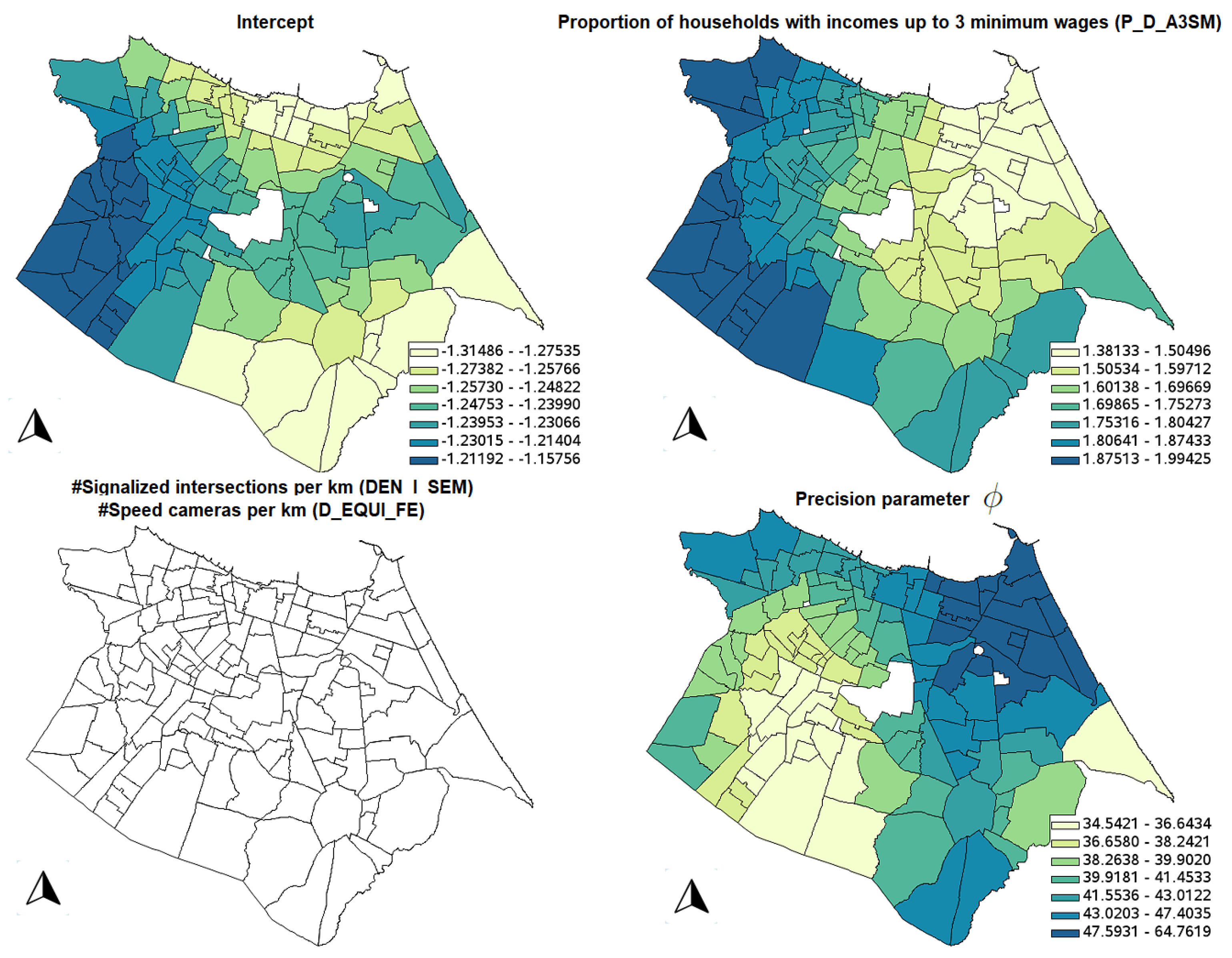
ENP	$8.96$

shows the descriptive statistics for the GWBR model. In the same fashion as the GWR model, Figure 5 shows the significant parameter estimates for the GWBR model; it is possible to see that all counterintuitive signs of the variables are not significant, considering the 10% significance level. Also, note that variables DEN_I_SEM and D_EQUI_FE are not significant in any location, but the spatial distributions of the other variables are smoother than in the GWR model. This is because GWR requires a smaller bandwidth to fit the data a little bit better compared to GWBR (compare the ENPs: 42.97 in GWR against only 8.96 in GWBR), generating an overfitted model (the same pattern is observed by [11] when GWPR is compared to GWNBR). With the spatial distribution of the GWBR coefficients, it is easier to understand the crash dynamics in the city.

Finally,

Table 8. Moran’s I for residual spatial dependence.

Model	Moran’s I	p-Value
Classical Linear Regression	$0.2594$	<$\hspace{0.25em}0.0001$
Beta Regression (logit)	$0.2354$	<$\hspace{0.25em}0.0001$
GWR	$-0.0500$	$0.1506$
GWBR (logit)	$0.1113$	$0.0329$

shows Moran’s I (using contiguity (Queen matrix) for the residuals of the models, indicating that there is spatial dependence in the global ones. In the local models, the spatial dependence is strongly reduced and it can be considered not significant for a 3% significance level, reinforcing the need for using a local model in the analysis.

3.3. Analysis of the Variable Traffic Injury (Fatal) Crash Proportions (${\mathrm{ACF}}_{\mathrm{P}}$)

As viewed before, the estimates of the classical linear regression model are quite different from those obtained by the beta regression with the logit link function (

Table 9. Results of the global models (dependent variable: ${\mathrm{ACF}}_{\mathrm{P}}$).

Variable	Classical Linear Regression			Beta Regression (Logit)
	Estimate	t	p -Value	Estimate	t	p -Value
Intercept	$-0.015936$	$-1.64$	<$\hspace{0.25em}0.1028$	$-5.553688$	$-13.52$	<$\hspace{0.25em}0.0001$
P_0_17	$0.1266574$	$3.81$	<$\hspace{0.25em}0.0002$	$6.0377913$	$4.50$	<$\hspace{0.25em}0.0001$
DEN_I_SEM	$-0.00590$	$-1.19$	$0.2346$	$-0.604053$	$-2.47$	$0.0149$
AREA_KM	$0.0011654$	$2.18$	$0.0311$	$0.023052$	$1.58$	$0.2040$
$\varphi$	-	-	-	$143.77925$	$7.58$	<$\hspace{0.25em}0.0001$
Adj $R^2$ *	$0.3212$			$0.5406$
AICc	$-710.7980$			$-825.9811$
log-likelihood	$359.5640$			$418.2406$

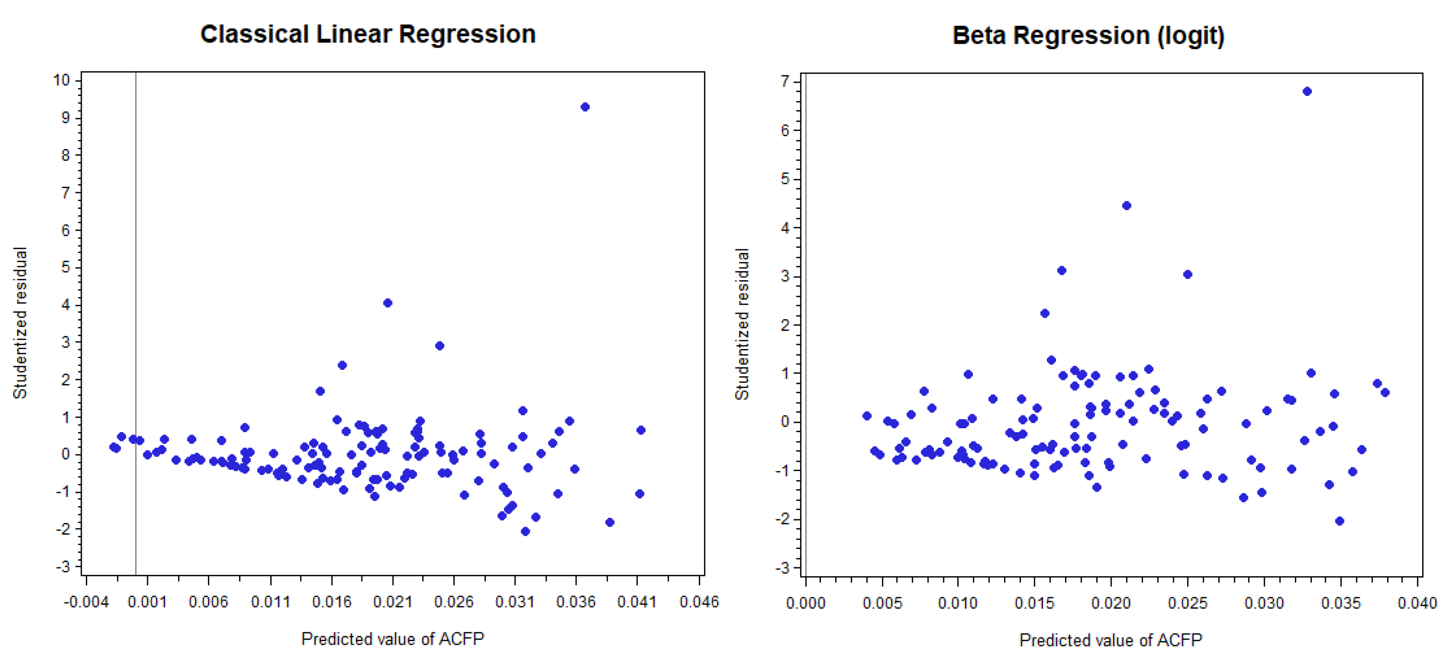
* Pseudo Adj R² for beta regression.

), but classical linear regression shows difficulty in fitting the data, primarily because they are not symmetric, as seen with the variable ${\mathrm{AC}}_{\mathrm{P}}$. First, the intercept being negative (when all observations of the variable ${\mathrm{ACF}}_{\mathrm{P}}$ are positive) is a strong indication that something is not right). For the beta distribution, this is not a problem because the predictions are made by using the exponential function. Second, the fact that the intercept is not significant (considering the 10% significance level) is another indication of a problem; it implies that when the variables P_0_17, DEN_I_SEM, and AREA_KM are zero, then there are no traffic injury (fatal) crashes, which is not true. Third, in Figure 6 classical linear regression produces some negative predicted values for the variable ${\mathrm{ACF}}_{\mathrm{P}}$. This behavior is not viewed in beta regression or with the variable ${\mathrm{AC}}_{\mathrm{P}}$ (because of the symmetry).

Also, all goodness-of-fit metrics were better in beta regression, and some variables showed opposite interpretations in relation to the significance: The variable DEN_I_SEM was considered not significant (for 10% significance level) in classical linear regression while it was highly significant in beta regression, and the variable AREA_KM was considered significant (for 10% significance level) in classical linear regression while it was not significant in beta regression. Because the assumption of symmetry required by classical linear regression was not met and the beta regression provided a better fit, we believe that the results from the beta regression are more reliable.

Similar to the variable ${\mathrm{AC}}_{\mathrm{P}}$, the best bandwidth found for the GWR model was an adaptive bandwidth when a CV was minimized, generating an adaptive bandwidth of 118 neighbors. And for the GWBR model, it was a fixed bandwidth when a CV was minimized, generating a fixed bandwidth of 20.4 km (or 20,413.27 m). In fact, these large bandwidths make GWR and GWBR models approximate to global ones, respectively. For comparison, the maximum distance between points was 21.6 km (or 21,617.91 m) and the maximum number of neighbors was 126.

Table 10. Descriptive statistics of the GWR model (dependent variable: ${\mathrm{ACF}}_{\mathrm{P}}$).

Variables	Coefficients
	Min	Q1	Median	Mean	Q3	Max
Intercept	$-0.0209$	$-0.0176$	$-0.0161$	$-0.0158$	$-0.0141$	$-0.0075$
P_0_17	$0.1033$	$0.1199$	$0.1269$	$0.1253$	$0.1314$	$0.1418$
DEN_I_SEM	$-0.0160$	$-0.0065$	$-0.0046$	$-0.0054$	$-0.0033$	$-0.0019$
AREA_KM	$-0.0002$	$0.0004$	$0.0006$	$0.0006$	$0.0008$	$0.0020$
Adj $R^2$	$0.3425$
Log-likelihood	$364.9303$
AICc	$-707.1279$
ENP	$10.34$

shows the descriptive statistics for the GWR model; Figure 7 shows the significant parameter estimates for the GWR model, using the test developed by [43]. It is possible to see that all counterintuitive signs of the variables were not significant, considering the 10% significance level.

Table 11. Descriptive statistics of the GWBR model (dependent variable: ${\mathrm{ACF}}_{\mathrm{P}}$).

Variables	Coefficients
	Min	Q1	Median	Mean	Q3	Max
Intercept	$-5.6546$	$-5.6210$	$-5.5933$	$-5.5868$	$-5.5556$	$-5.4792$
P_0_17	$5.8129$	$6.0386$	$6.1459$	$6.1320$	$6.2425$	$6.3690$
DEN_I_SEM	$-0.6457$	$-0.6104$	$-0.5979$	$-0.6013$	$-0.5905$	$-0.5751$
AREA_KM	$0.0203$	$0.0212$	$0.0217$	$0.0218$	$0.0224$	$0.0234$
$\varphi$	$138.5076$	$147.0267$	$149.9394$	$149.1955$	$152.3007$	$156.9339$
Pseudo adj $R^2$	$0.5461$
Log-likelihood	$419.7047$
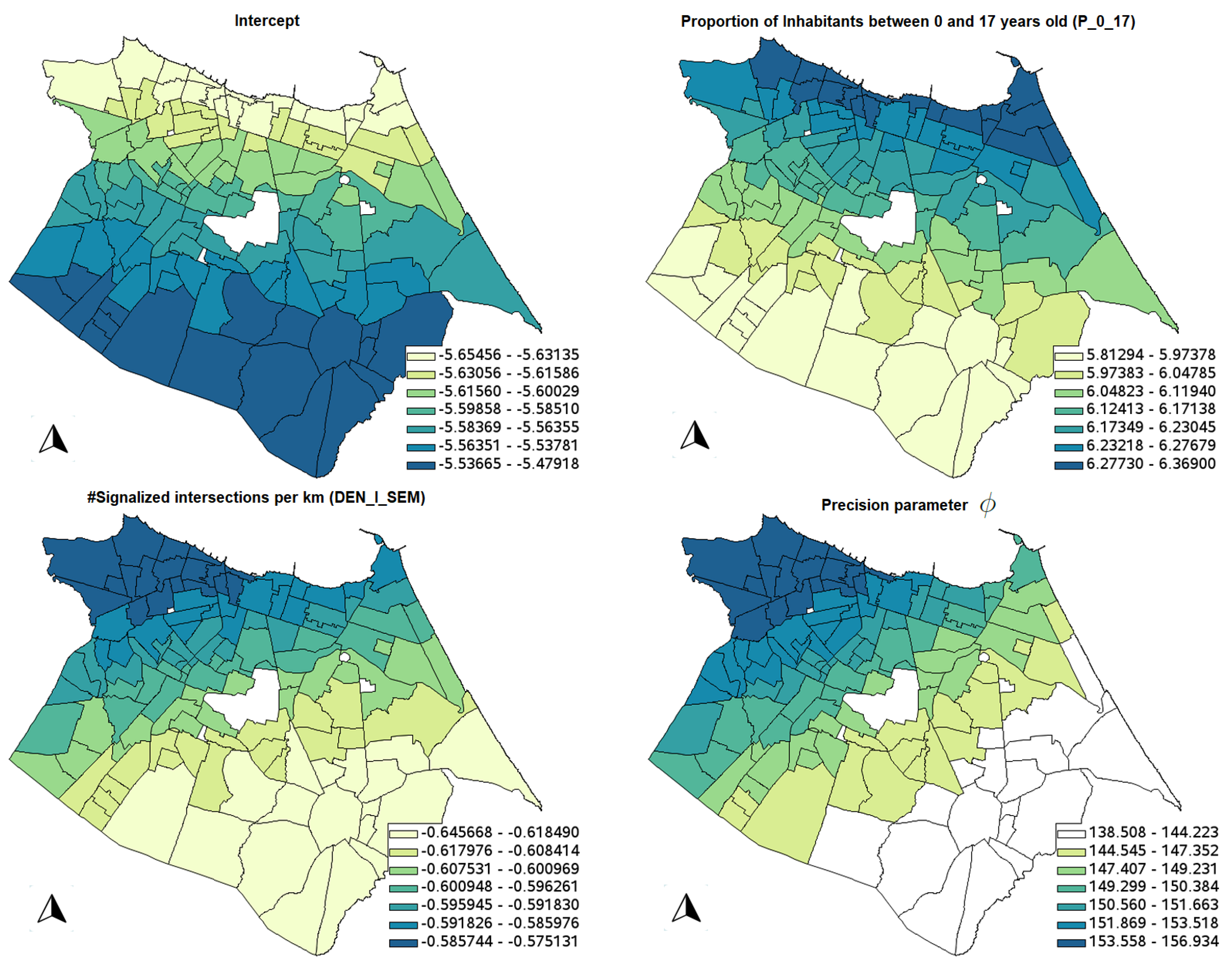
AICc	$-830.1279$
ENP	$4.36$

shows the descriptive statistics for the GWBR model and Figure 8 shows the significant parameter estimates for the GWBR model. It is possible to see that all counterintuitive signs of the variables were not significant, considering the 10% significance level; moreover, the variable AREA_KM was not significant in any location (not shown in the figure). Again, the same smoother distribution of the parameter estimates is observed in the GWBR model.

Finally,

Table 12. Moran’s I for residual spatial dependence.

Model	Moran’s I	p-Value
Classical Linear Regression	$-0.0403$	$0.1946$
Beta Regression (logit)	$0.0191$	$0.4218$
GWR	$-0.0772$	$0.0645$
GWBR (logit)	$-0.0187$	$0.3169$

shows Moran’s I (using a contiguity Queen matrix) for the residuals of the models, indicating that there is no spatial dependence in the global ones. However, the local models were fitted to data and the residual also showed no spatial dependence, as expected. This result shows the ability of the GWBR model to fit data with or without spatial dependence, making the GWBR model the only necessary model for the analysis of rates or proportions.

4. Conclusions

This study investigated the use of geographically weighted beta regression (GWBR) for estimating traffic injury crash proportions at the traffic zone level, based on a case study in Fortaleza, Brazil. In traffic modeling literature, the use of classical linear regression (or its spatial local version, GWR) for modeling rates or proportions is common, as the data are continuous. However, as seen in this work, the results support the use of beta regression (or, more effectively, its spatial local version GWBR) as a promising tool for safety planning, since it can handle symmetric and skewed distributions, as well as spatial and non-spatial data, without any transformation of the data (unlike some studies that use a log transformation to achieve normality).

The R package, named ‘gwbr’, developed by the authors, facilitates the use of this new technique in transportation planning to more effectively model rates or proportions, such as fatal traffic injury crash proportions. The results showed that when the data distribution is asymmetric, the beta distribution provides a superior fit compared to classical linear regression. When the distribution of data is approximately symmetric, the beta distribution still shows an apparent superior adjustment to classical linear regression. This facilitates the modeling task since it is not necessary to find the normality (or symmetry) of the data.

To the best of our knowledge, this study is the first application of the GWBR model to the field of road safety. The main contribution of this work, based on the results, is the recommendation to use the GWBR model when analyzing rates or proportions. This model effectively fits both symmetric and skewed distributions limited to the interval (0,1), with or without spatial dependence.

A clear limitation in using GWBR concerns the use of the extremes of the interval (0, 1), i.e., 0 and 1. When we have locations with 0% traffic injury crashes, which is highly desired, the data should be replaced by a number close to zero. Furthermore, if the distribution shows a lot of zeros, which is also highly desired, a zero-inflated version of the GWBR model is recommended, but this model has not yet been developed. These points require further investigation in the future.