Data-Driven Prediction of Stability of Rock Tunnel Heading: An Application of Machine Learning Models

Abstract

In this paper, Artificial Neural Networks (ANN) have been utilized to predict the stability of a planar tunnel heading in rock mass based on the well-defined Hoek-Brown (HB) yield criterion. The HB model was developed to capture the failure criterion of rock masses. To provide the datasets for an ANN model, the numerical upper bound (UB) and lower bound (LB) solutions obtained from the finite element limit analysis (FELA) with the HB failure criterion for the problem of tunnel headings are derived. The sensitivity analysis of all influencing parameters on the stability of rock tunnel heading is then performed on the developed ANN model. The proposed solutions will enhance the dependability and preciseness of predicting the stability of rock tunnel heading. Note that the effect of the unlined length ratio has not been explored previously but has been found to be of critical importance and significantly contributes to the failure of rock tunnel heading. By utilizing the machine learning-aided prediction capability of the ANN approach, the numerical solutions of the stability of tunnel heading can be accurately predicted, which is better than the use of the classic linear regression approach. Thus, providing a better and much safer assessment of mining or relatively long-wall tunnels in rock masses.

1. Introduction

In tunnelling and mining works, the safety assessment of underground spaces is crucial to ensure stability during the construction process. Precise and efficient analysis for predicting tunnel face stability is required in order to minimize ground movements and risk of failure in tunnel constructions.

The plastic bounds theorems Drucker et al. [1], the finite element idea Zienkiewicz et al. [2], and the notion of perfectly flexible material with an accompanying flow rule are all applied in finite element limit analysis (FELA) in accordance with the mathematical programming initially used by Sloan and Assadi [3]. They have applied these approaches to analyze the problem of 2D tunnel headings face stability in homogeneous clays, offering upper bound (UB) and lower bound (LB) solutions. By employing the FELA approach, Augarde et al. [4] investigated the effects of non-homogeneity of face stability in 2D tunnel head problems. The plastic solutions of 2D tunnel headings in cohesive-frictional soils and undrained heterogeneity clay were also provided by Yang et al. [5] and Huang and Song [6] respectively. The stability problem of d planar tunnel headings and circular tunnels in anisotropic and non-homogeneous clays was recently explored by Ukritchon and Keawsawasvong [7] and Keawsawasvong and Ukritchon [8]. The solutions to a similar problem of the stability of the retaining soils behind openings in subterranean walls were also carried out by Ukritchon and Keawsawasvong [9,10]. However, these studies were limited to tunnel stability obeying the Mohr-Coulomb (MC) model that is suitable only for sand and clay media.

In the 1980s, the Hoek-Brown (HB) failure criteria Hoek and Brown [11] was formulated by gathering data from the triaxial test of entire and welded rocks based on the curve fitting technique. Unlike the MC model, where the internal frictional angle and the cohesion are the parameters that represent the soil properties, more input parameters are required in the HB model to be able to capture the nonlinear rock masses’ shear strength as well as the various important aspects of their failure behavior. In 2002, Hoek et al. [12] developed the original HB model to accommodate extremely fragmented media. The mathematical framework of the model may be stated as a power-law function in terms of the major and minor principal stresses, which according to Hoek et al. [12]’s updated formulation of the HB failure yield criterion, can be simplified as:

$$\hspace{0.17em}{\sigma }_3={\sigma }_1-{\left(-m_b{\sigma }_1{(-{\sigma }_{ci})}^{(1-a)/a}+s{(-{\sigma }_{ci})}^{1/a}\right)}^a$$

(1)

where σ₁ represents the major principal stresses while σ₃ represents the minor principal stresses. In addition, σ_ci stands for the uniaxial compressive strength of whole rocks. Note that the parameters m_b, s and a are expressed in the following relationships:

$$m_b=\hspace{0.17em}{m}_i\exp \left(\frac{GSI-100}{28-14DF}\right)$$

(2)

$$s=\hspace{0.17em}\exp \left(\frac{GSI-100}{9-3DF}\right)$$

(3)

$$a=\frac{1}{2} + \frac{1}{6}\left(e^{-\frac{GSI}{15}}-e^{-\frac{20}{3}}\right)$$

(4)

According to previous equations, the GSI (Geological Strength Index) parameter describes the discontinuities’ surface condition, and the rock’s structural composition both have a significant influence on the physical characteristics of rock masses. The GSI classification ranges from 10 (extremely poor laminated/shear rock masses) to 100 (very good intact or massive rocks). The DF parameter describes the level of rock mass disruption caused by explosion impact and stress relaxation on rock masses, with a range of 0 (the quality of the rock is undisturbed) to 1 (the quality of the rock is highly disturbed). Rock parameter m_i represents the rock mass’ frictional strength in which the values of this parameter are affected by a variety of variables, including grain size and mineral content. The HB yield criterion was developed and has been implemented in several numerical and analytical techniques to create stability solutions to a variety of challenges, such as the stability analyses of rock slopes [13,14,15,16,17], underground openings [18,19,20,21,22,23], and the bearing capacity of footings [24,25,26,27,28,29,30,31,32,33,34,35,36].

For previous studies of rock tunnel stability using FELA, Ukritchon and Keawsawasvong [37], Keawsawasvong and Ukritchon [38] and Xiao et al. [39] employed the FELA to offer stability solutions for various shapes of tunnels in HB rock masses which consists of a square, circular, and rectangular tunnel, respectively. Xiao et al. [40], Zhang et al. [41] and Rahaman and Kumar [42] also utilized FELA in combination with the Hoek-Brown yield criterion to compute the stability solutions of the dual square, dual circular, and dual horseshoe tunnels, respectively. For the problem of planar tunnel heading, which correlates to a simulation of an endlessly infinite tunnel or underground mining, the work by Ukritchon and Keawsawasvong [43] was only of consequence. However, Ukritchon and Keawsawasvong [43] did not consider an unlined length ratio of the headings and only LB solutions were presented in their study. It is worth noting that the unlined length ratio of tunnels has a substantial impact on the reduction of tunnel stability, as demonstrated by Sloan [44] and Shiau and Al-Asadi [45]; nevertheless, the impact of this variable on rock tunnels has not been studied. Furthermore, the aforementioned analyses on rock tunnel stability were only introduced in terms of tables and charts, which made it complicated to apply directly for arbitrarily defined values of all analyzed parameters, including the HB parameters or tunnel shape, without the usage of the solution’s estimation or interpolation.

An artificial neural network (ANN) is a computational strategy that gathers and learns from a significantly sufficient database and then establishes a black-box-type prediction model to address a range of problems in terms of a closed-form equation. Its predictive capability through the learning and training process was discovered to be a crucial indicator in treating a number of geotechnical issues. The ANN-based models have been presented by [46,47,48,49] to estimate the ultimate bearing capacity of foundations on rock masses. It has also been employed by Li et al. [50] to perform the rock inclination stability prediction by a terminal steepest descent technique with an extreme learning neural network, where a training set of FELA results was applied. In addition, the soft computing of tunnel stability problems was also considered by Naghadehi et al. [51] and Ghorbani et al. [52] for tunnels in cohesive-frictional soils and rock masses, respectively. Published papers by Lee et al. [53] and Mahdevari et al. [54] and most recently, Keawsawasvong et al. [55] have utilized the ANN technique to check the stability of tunnels through prediction of final displacement, convergence and face support pressure, respectively. [56,57,58,59] also employed the same soft computing method to predict the stability of various tunnel shapes through a parametric study. More details on the application of machine learning algorithms in geotechnical engineering can be found in [60,61,62,63].

This paper highlights for the first time the important aspect of considering the effect of the unlined length ratio in the prediction of rock tunnel heading stability. A soft computing (i.e., ANN method) tool is employed to evaluate the database and produce a predicted output for the problem of the rock tunnel heading stability for the first time. The practical solution developed in this work, which is predicated on the ANN technique, not only offers a rapid evaluation of tunnel stability in rock mass which can be applied to long-wall tunnels or underground mining construction but also improves the accuracy and reliability of the stability calculation of plane strain tunnel heading problem in HB rock masses. Please note that the rapid nature of the evaluation is mainly due to the surrogate model developed from the trained ANN/multivariate linear regression. Thus, the surrogate model based on the ANN technique can provide a better and much safer assessment of mining or relatively long-wall tunnels in rock masses.

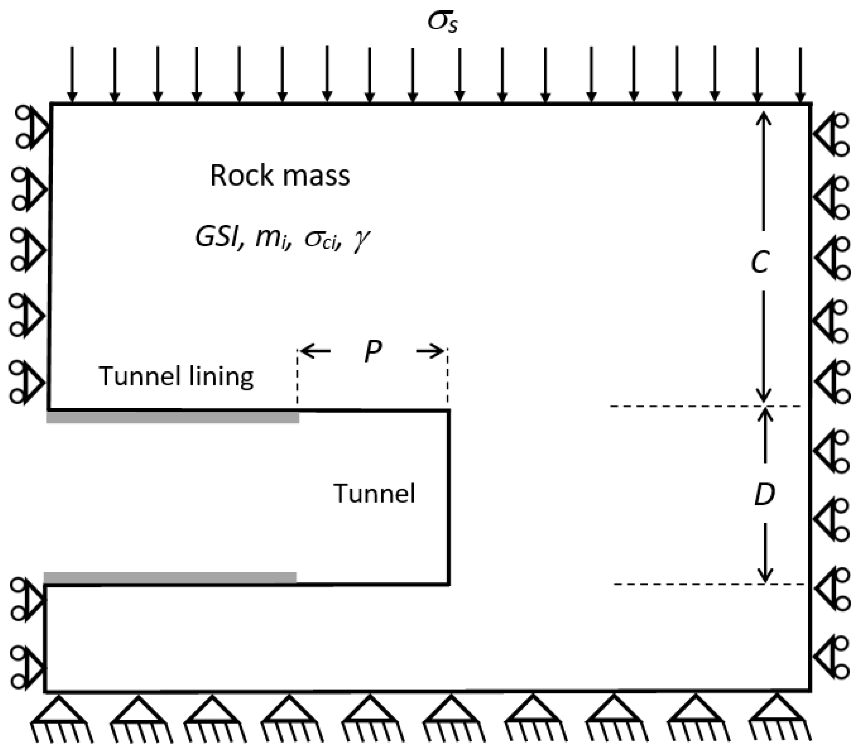
2. Problem Statement

The problem description of a plane strain tunnel heading with an unlined length is shown in Figure 1. Since the problem is defined to be under the plane strain condition, a three-dimensional subsurface excavation or tunnel wall along the longitudinal plane is represented by the plane strain heading. The rigid lining is placed in both the upper and lower part of the heading, where an unlined length (P) is located between the end of the rigid lining and the tunnel face. The tunnel’s geometry includes a height (D) located at a cover depth (C). A surcharge loading (σ_s) with a uniform distribution is delivered from the surface of the rock mass. This loading enables the front face of the tunnel to collapse, as well as the entire length of the tunnel heading. The rock mass is defined under the assumption of the HB yield criterion with the HB parameters as mentioned in Equations (1)–(4).

The surrounding rock mass is assumed to remain undisturbed throughout the tunnel construction. As a result, the undisturbed in-situ condition is applied in all analyses by setting the disturbance factor DF = 0. By employing the dimensionless analysis technique Butterfield [64], the relationship between five dimensionless input variables and one dimensionless output variable of this problem can be expressed as:

$$\frac{{\sigma }_s}{{\sigma }_{ci}}=f(\frac{C}{D},\frac{\gamma D}{{\sigma }_{ci}},\frac{P}{D},GSI,m_i)$$

(5)

where

σ_s/σ_ci denotes the stability factor;

C/D denotes the cover depth ratio;

γD/σ_ci denotes the normalized uniaxial compressive strength;

P/D denotes the unlined length ratio;

GSI denotes the geological strength index;

m_i denotes the HB material constant in relation to the frictional strength.

The values of all dimensionless input parameters investigated are listed in Equation (5). To obtain the machine learning models, the output dataset is considered to be the stability factor calculated by FELA solutions. It is crucial to highlight that these variations shown in Equation (5) include all possible geometries of tunnels and rock mass characteristics based on previous articles by [37,38,39,40,41,42,43]. These data will be used to calculate the stability factor using FELA in Section 3 and also be used in conjunction with the corresponding results obtained from FELA to create machine learning models at a later stage.

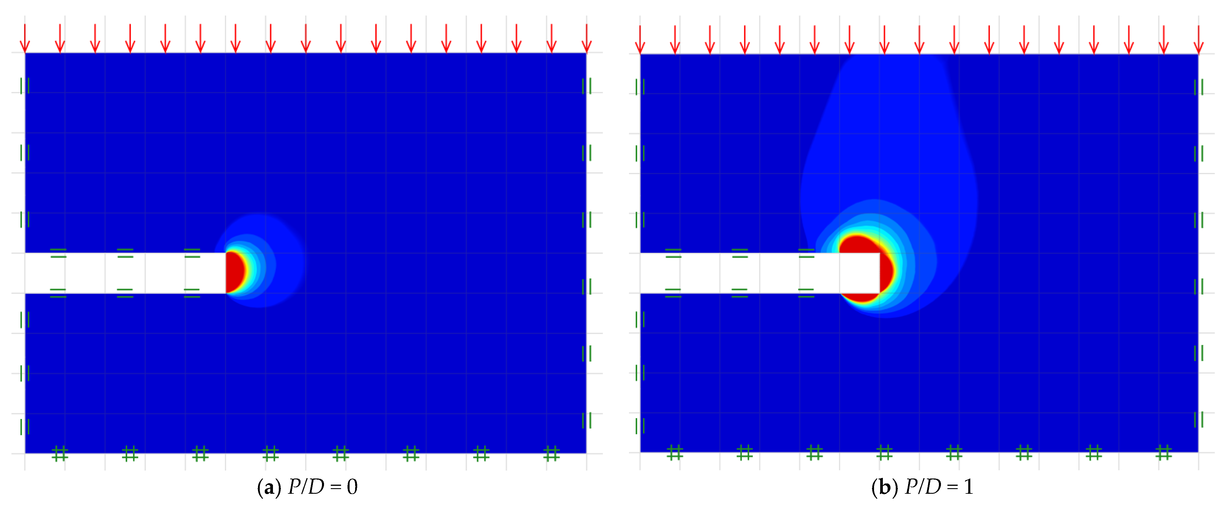
3. Finite Element Limit Analysis (FELA)

The surface pressure (σ_s) of plane strain tunnel headings with an unlined length in rock masses is computed using a modern FELA program, OptumG2 [65]. The FELA provides a computer approach for handling a perfectly plastic material with an accompanying flow rule [66,67,68,69,70,71,72,73,74,75,76]. This FELA can be used to limit the surface pressure (σ_s) between the desired UB and LB solutions. Average bound solution outcomes are utilized as datasets to develop machine learning models based on a neural network and an extreme learning algorithm.

The stability solutions of plane strain tunnel headings are presented in this study using the OptumG2 FELA software. This FELA is a highly potent numerical method that combines the utilization of finite element discretization techniques together with specified boundary conditions within the perspective of plastic-bound theorems. Based on the establishment of UB analysis, the domain of the slopes is discretized into a limited number of six-noded triangular elements. Within the triangle element, each node includes two unidentified velocities. The UB approach can minimize the surface pressure of tunnels (objective function), utilizing optimization problems with constraints related to the velocity boundary conditions and compatibility equations. Based on LB analysis, the discretized tunnel domain consists of several triangular components with three nodes, each with three unidentified stresses. A stress field in the LB formulation is produced to be consistent inside the triangular element by employing an individually linear variation. In the LB approach, discontinuities across the overlapping edges of adjacent elements are permitted. The optimization method is also necessary for LB calculations. The equilibrium equations for the triangular element and across stress discontinuities serve as the basis for the statically acceptable stress field restrictions in LB analysis. The surface pressure of tunnels is then maximized, which is the objective of the optimization process in the LB approach.

In Figure 2a–c, three typical numerical model geometries of this problem are demonstrated for the cases of the unlined length ratio P/D = 0, 1 and 2, respectively, while other parameters are set to be C/D = 5, m_i = 30, GSI = 40, and γD/σ_ci = 0.01. For the left and right boundaries, a standard boundary condition is applied in which the movements are just permitted in the vertical plane. At the bottom, a fully fixed support is applied where both motions in vertical and horizontal planes are prohibited. At the ground surface of the problem, the uniformly distributed pressure σ_s is applied over the plane. At the top and bottom linings, roller supports are defined at both planes, so that horizontal motions are permissible except at the top and bottom unlined lengths, which are set to be free surfaces. Note that the domain sizes should be huge enough to eliminate any potential undesirable effects of the problem size on the generated bound solutions. To obtain the bound solutions, the pressure σ_s during the active collapse event is optimized by using OptumG2 and then normalized to render the stability factor σ_s/σ_ci that is considered to be a function of the five dimensionless parameters presented in Equation (5).

To enhance the precision and accuracy of the generated bound solutions, the adaptive meshing technique based on the scheme originally introduced by Ciria et al. [77] is activated in all numerical analyses. Accordingly, the number of elements is effectively raised in zones with substantial plastic shear strains, considerably improving the computational accuracy of all simulations. Nonetheless, increasing the number of elements and consequential increase in the generated data set only applies to zones of significance in order to keep the computational cost as low as possible. After a few iteration steps, there are fewer disparities between UB and LB solutions, thus yielding tighter UB and LB solutions. In this study, the adaptive meshing method is set up so that in the first stage, an initial mesh of typically 5000 elements is formed, followed by three phases of mesh adaptivity to reach a final mesh of 10,000 elements. The examples of typical adaptive meshes after three iteration steps for the cases of P/D = 0, 1 and 2 are shown in Figure 3a–c, respectively. Moreover, Figure 4a–c demonstrates examples of absolute velocity contours for the same cases as Figure 2 and Figure 3. It can be seen that Figure 3 and Figure 4 depict similar failure mechanisms of rock tunnel heading, where the number of elements is dramatically raised in the failure zones with high absolute velocity contours. By applying the FELA and the adaptive meshing technique with the same setting as shown in Figure 3, all 960 results from average bound solutions are acquired. The datasets obtained from these solutions are then employed in the machine learning techniques, which are outlined later in the next section. Note that Sloan [44] stated that the stability analysis using the FELA based on the limit analysis theory requires only the conventional strength parameters, such as undrained shear strength, but does not use the deformation parameters, such as Poisson’s ratio and Young’s modulus which is different from the conventional displacement-based FEM. Thus, Poisson’s ratio and Young’s modulus are not considered in this study. Hence, large deformations of rock tunnels cannot be investigated by using FELA.

4. Machine Learning

4.1. Database

In the database, there are five input data attributes related to the tunnel geometry and soil conditions that are presented in

Table 1. Input parameters.

Input Parameters	Values	Average
C/D	1/2/3/4/5	3
P/D	0/0.5/1/2	0.875
GSI	40/60/80/100	70
mi	5/10/20/30	16.25
γD/σci	0/0.001/0.01	0.0037

. The output data is the stability factor that has been calculated based on FELA. The range of the stability factor is shown in

Table 2. Output parameter.

Output Parameter	Values	Average
σs/σci	0.0415-98.9825	10.2643

. The input parameters and corresponding results are then organized to formulate machine learning models. In this study, there are 960 datasets that could be used for creating machine learning models. The data of stability factor calculation contains two parts for training and testing sets. The cross-validation is then performed on the training set, which contains 80% of the completed dataset to prevent overfitting, while the remaining 20% is used to test the model and evaluate the performance of the developed model.

4.2. Multiple Linear Regression (MLR)

The approach of modeling the linear correlation between the scalar outcomes (outputs referred to as dependent variables) and informative variables (inputs referred to as independent variables) is known as linear regression. If there is just one independent variable in the correlation, a simple linear regression is performed. Since there are five independent variables in this analysis, the technique is known as “multiple linear regression”, which is among the most outstanding and simplest methods in regression issues. Furthermore, Gomes et al. [78] effectively utilized this strategy in forecasting pile-bearing capacity as a baseline performance of the machine learning model.

From the linear function combining all input or independent variables, the output, which is a dependent variable, can be computed by using the below equation.

$$y_i={\beta }_0+{\beta }_1{x}_{i1}+{\beta }_2{x}_{i2}+\dots +{\beta }_p{x}_{ip}+ϵ$$

(6)

where

$y_i$ = dependent variable (output);

$x_{i1}, x_{i1}, \dots x_{ip}$ = independent variables (inputs);

${\beta }_0$ = y-intercept (constant term);

${\beta }_1, {\beta }_1,\dots , {\beta }_p$ = slope coefficients for each explanatory variable;

$ϵ$ = the model’s error term (also known as the residuals).

According to the regression function described earlier, a linear correlation between the output variable y and the p-vector of regressors x is observed. An error variable, often known as a residual term, is an undetected random variable that reflects the function’s noise. This study uses a public program called WEKA (Waikato Environment for Knowledge Analysis), established by the University of Waikato, New Zealand. It is a set of machine learning techniques for data mining tasks that includes data pre-processing, categorization, regression, grouping, affiliation rules, and dashboards for data analysis and predictive modeling.

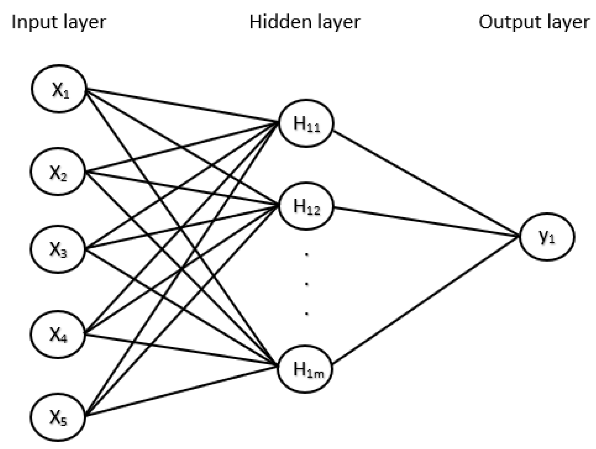
4.3. Artificial Neural Network (ANN)

An Artificial Neural Network (ANN) is additionally employed in this paper. This technique offers a platform for data interpretation predicated on inherent characteristics obtained from the composition of the human intellect. It replicates the neurological processes used by the human brain to process complicated data. An enormous number of linked nodes (or neurons) compose the computer model known as a neural network. An ANN model has three layers, including the output, hidden, and input layers (see Figure 5). The feature vector is transmitted through the input layer. We configured the input layer to contain five nodes signifying C/D, P/D, γD/σ_ci, GSI and m_i. For the second layer, which is called the hidden layer, it involves a single or many layers of threshold logic units. Normally, a trial-and-error method is employed to find out the number of hidden layers as well as the hidden neurons in order to obtain the best values of them. Note that the best model of hidden layers can yield the utmost prediction of output data by turning an input into the content and anticipating data. The weighted sums of the inputs may also be produced within this layer, in which a step function can be implemented before being transmitted out as an output utilizing the sigmoid activation function. The learning rate is set to 0.3, which is acceptable in this case. Finally, the output layer is the dependent variable or a predicted value after passing through those first and second layers. Since there is only one output which is a predicted stability factor of the plane strain tunnel heading in the rock mass, this final layer has only one node.

4.4. 10-Fold Cross-Validation

Since there is a minimal amount of information, the partitioning strategy into training and testing datasets can be inaccurate. A highly comprehensive approach for countering such a bias caused by the particular sample that can be exploited for persistence is to repeatedly perform the entire procedure of testing and training, employing randomized produced samples. Stratification by tenfold cross-validation is a method frequently used to validate machine learning approach models. In this paper, 80% of the dataset is used for the training set and tenfold cross-validation to avoid overfitting. With the category provided roughly the same percentages as the overall training dataset, the datasets are divided into 10 segments at random. Each segment is carried out in turn, the remaining nine-tenths are then examined, and finally, the holdout set’s error rate is assessed. The learning operation is consequently carried out 10 times on various training sets. Finally, the entire forecast error is subsequently calculated by averaging the last 10 errors.

4.5. Performance Measures

Three statistical methods, the correlation coefficient (R), the mean absolute error (MAE), and the root mean squared error (RMSE), are employed to assess the efficiency of trained models in this paper. Correlation coefficients are used to quantify the statistical relationship between expected and actual values of a certain parameter. Correlation coefficients vary from 0 (no correlation) to 1 (perfect correlation). Notably, a correlation value lower than zero represents a negative correlation. It is different from the other metrics in that it is scale-independent, which implies that for a particular set of forecasts under evaluation, if a constant multiplier is applied to each and every prediction, the error remains unchanged. Meanwhile, as opposed to the other measures, the actual values also remain unchanged. Indeed, this constant factor really exists in both the numerator and denominator of each phrase of S_PA and S_P, respectively, thus cancelling out—See Equation (7). Although the relative error figures have been adjusted, this is not the case since all forecasts are multiplied by a sizable constant. Thus, the discrepancy between the actual and expected values widens considerably, as well as the error percentage. Additionally, it is distinct in that the results of high performance are indicated by a big correlation coefficient, while, on the other hand, high efficiency is signified by small values in the other error measuring techniques such as MAE and RMSE.

$$R=\frac{S_{PA}}{\sqrt{S_P{S}_A}}$$

(7)

where

$S_{PA}=\frac{{{\displaystyle \sum }}_i\left(p_i - \overline{p}\right)\left(a_i - \overline{a}\right)}{n - 1},$$S_P=\frac{{{\displaystyle \sum }}_i{\left(p_i - \overline{p}\right)}^2}{n - 1}$, $S_A=\frac{{{\displaystyle \sum }}_i{\left(a_i - \overline{a}\right)}^2}{n - 1}$

$\overline{p}$ and $\overline{a}$ are the average values of p and a variables, respectively.

n is the number of datasets.

The square of the correlation coefficient is known as the determination coefficient (R-squared, R²). Remember that R cannot fully represent the strength when there is more than one variable or several linear regressions are taken into consideration. Hence, in the situation of multiple variables, R² can be a better indication for this established model. Thus, R² is one of the metrics utilized to assess the performance of machine learning models.

Moreover, Mean Absolute Error (MAE) represents the mean value of the particular errors that do not consider the sign convention. Moreover, Mean-Squared Error (MSE) represents a general and most common method for error measurement. It does, however, accentuate the influence of outliers (cases where the forecast inaccuracy is greater than the others), while absolute error does not. All error sizes are considered equally based on their magnitude. The expression for MAE calculation is shown in Equation (8).

$$MAE=\frac{\left|p_1-a_1\right|+\dots +\left|p_n-a_n\right|}{n}$$

(8)

Although MSE is the approach that is most frequently employed, the square root (Root Mean Squared Error, or RMSE) is also occasionally adopted to get equivalent dimensions to the dependent variable. However, in evaluating and contrasting the efficiency of a regression model with other random models, RMSE is more frequently used than MSE. The expression for RMSE calculation is shown in Equation (9).

$$RMSE=\sqrt{\frac{{\left(p_1-a_1\right)}^2+\dots +{\left(p_n-a_n\right)}^2}{n}}$$

(9)

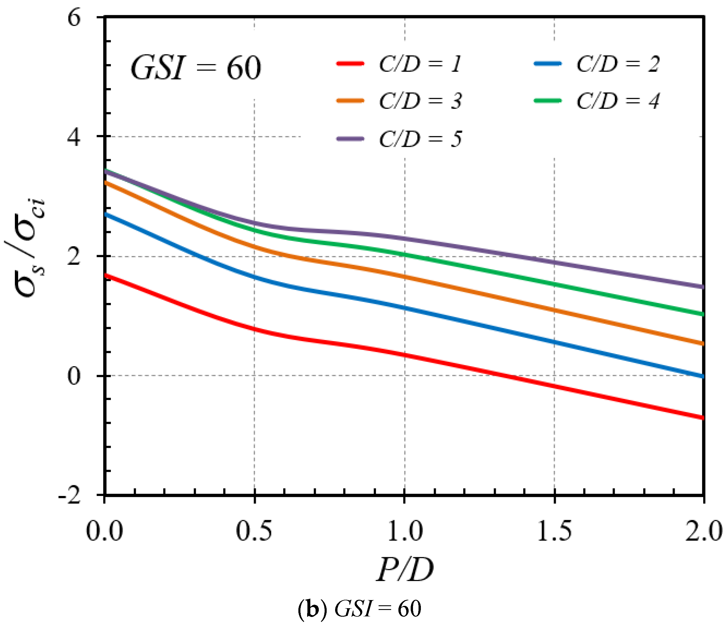
5. Results and Discussions

After employing the Multiple Linear Regression (MLR) and Artificial Neural Network (ANN) as described in the previous sections, the stability of a planar tunnel heading in rock mass based on the Hoek-Brown (HB) yield criterion can be predicted using those models. The multiple linear regression equation is first presented, followed by the employed ANN models. Next, the performance of MLR and ANN models is discussed. As for ANN models, the proposed model is developed with constant values, including bias and weight matrices that can be used to form an equation. Afterwards, the results between the proposed ANN model and the past work are compared. Lastly, the sensitivity analysis result is performed to clearly illustrate the influences of each input factor on the stability factor of rock tunnel heading.

5.1. Multiple Linear Regression (MLR)

Firstly, while utilizing WEKA software, the regression coefficients of each explanatory variable are optimized by reducing error. The stability factor’s prediction equation predicated on multiple linear regression is shown in Equation (10).

$$y=2.8761x_1-6.4631x_2+0.3301x_3+0.5840x_4-2.392x_5-25.3011$$

(10)

where $y$ denotes as the stability factor (σ_s/σ_ci) whereas $x_1,x_2,x_3,x_4,and x_5$ represents the dimensionless input parameters which consist of C/D, P/D, GSI, m_i, and γD/σ_ci, respectively. The developed equation’s performance can be assessed via statistical tests, i.e., R², MAE and RMSE, which are determined to be 0.6313, 5.7526 and 8.5310, respectively (see

Table 3. Performance measures of each methodology.

Methodology	R2	Mean Absolute Error (MAE)	Root Mean Squared Error (RMSE)
Multiple Linear Regression (MLR)	0.6313	5.7526	8.5310
Artificial Neural Network (ANN)	0.9982	0.6204	0.7740

).

5.2. Artificial Neural Network

To increase the predictive ANN models’ efficiency and predictability, it is recommended that the number of hidden layers and neurons should be enhanced. The performance evaluation of the models versus the number of hidden neurons is shown in Figure 6. It is obvious that ANN models operate better as the hidden neurons increases. However, above a certain threshold value, it has been discovered that increasing the number of neurons does not significantly boost the model’s accuracy. It is also revealed that when the number of hidden neurons in an ANN model exceeds 9, the performance tends to stabilize. In this study, the best ANN model is proposed to be 5-9-1 architecture according to the statistical results compared to other architectures. The effectiveness of the MLR and ANN models is compared in Table 3. Clearly, the ANN model outperforms the MLR model, which seems to be less effective for this case model. The succeeding part will conduct a sensitivity analysis using this ANN model with a 5-9-1 architecture. Figure 7 compares the FELA solutions with the ANN model results. As shown, the ANN model is capable of accurately predicting the stability factor of a rock tunnel heading with an unlined length.

The estimation general functions may be employed to develop outputs by accounting for the weighted inputs and the transfer function upon choosing the optimum ANN architectural design. To simulate general functions, this network may be employed. If the hidden layer has enough neurons, it can infinitely well anticipate any function with a finite number of discontinuities. In order to identify how each parameter affects the stability factor, the ultimate weights for each parameter are established in this section. The best ANN model for forecasting the stability of rock tunnel heading is shown in Figure 8, alongside the dimensions of the input, weight, bias, and output matrices. Therefore, using the matrices obtained from the ANN model, the prediction equation can be formed as shown in Equation (11).

$$Predicted value=\left[{{\displaystyle \sum }}_{i = 1}^{N}IW{2}_{i}tansig({{\displaystyle \sum }}_{j=1}^{J}IW{1}_{ij}{x}_j+b_{1i})+b_2\right]$$

(11)

where x represents the input variables; J reflects the number of input variables, N represents the number of hidden neurons. In the hidden and output layers, IW1 and IW2 stand for the weight matrices, and b_1i and b₂ are the bias, respectively, associated with proposed ANN models. The quantity of hidden neurons (N) and input parameters (J) determine the adoption of a hidden weight (IW1). The output matrix comprises just one column in this situation. With regards to the input weight matrix (IW2), it has the same number of rows as the number of hidden neurons (N), and its column count equals the number of output (k), with one column for each neuron in the output layer. In addition, it has one column for each neuron in the hidden layer. As shown in

Table 4. Neural network constants.

Hidden Layer Neurons (i)		Hidden Layer Bias (b1)	Hidden Weight (IW1)
			C/D (j = 1)		P/D (j = 2)	GSI (j = 3)		mi (j = 4)	γD/σci (j = 5)
1		−5.0733	−1.6658		−0.6023	1.3245		0.7760	0.0138
2		−1.8481	−0.0550		0.1802	0.0961		−0.0057	0.2143
3		−1.5341	−0.0605		−0.1463	−0.5307		−0.1405	0.0254
4		−1.8298	0.1549		−0.1237	0.3186		0.0550	0.2366
5		−3.4584	0.5283		−0.4715	1.6357		0.5328	0.0120
6		−1.9151	−0.0534		0.3226	0.2164		0.0401	0.0842
7		−4.5532	0.6104		−0.8435	1.2468		−1.3417	0.0172
8		5.2780	−0.1685		2.2840	−1.2978		−0.7315	−0.0087
9		−1.7423	−0.0802		0.3572	0.3623		0.0068	−0.0326
Output layer node (k)	Output layer bias (b2)	Output weight (IW2)
		i = 1	i = 2	i = 3	i = 4	i = 5	i = 6	i = 7	i = 8	i = 9
1	−1.6224	−0.1079	−0.5422	0.2435	2.5051	−0.2877	−1.1940	−2.8165	−0.5377	−1.6224

, the constants of the ideal ANN network, which includes the weight and bias matrices, are used to calculate the stability factor of tunnel headings with an unlined length. It is possible to utilize the values produced from the best ANN network to construct predictive equation functions, which can then be tested on fresh datasets with various changes in data ranges.

5.3. Verification

The differences between the computed UB and LB FELA solutions with the adaptive meshing technique and the HB yield criterion are less than 5% for all 960 computed results. Thus, all numerical results presented hereafter are the average bound solutions (Ave), which are employed as the training datasets in the ANN model as described earlier. To verify the present scheme, Figure 9 demonstrates a comparison of the stability factor (σ_s/σ_ci) between the solutions from the present ANN model and those reported by [43]. Since the solutions by [43] are limited to the cases of P = 0, the chosen set of parameters for comparison includes: P/D = 0; m_i = 20; γD/σ_ci = 0.01; GSI = 40, 60, 80, 100; and C/D = 1, 2, 3, 4, 5. Figure 9 demonstrates that the present solutions are generally greater compared to the ones reported in the previous study. This is because the solutions by [43] reported only the LB results, while the present study is based on the average. Nevertheless, the general trends of the two solutions indicate a significant degree of agreement. Therefore, this comparison can boost further confidence in the approach and can confirm the high accuracy of the present ANN model considerably before proceeding to the sensitivity analysis in the next section.

5.4. Sensitivity Analysis

The purpose of this section is to illustrate the impact of all input factors in Equation (5) on the stability factor by conducting a sensitivity analysis on the stability of plane strain tunnel headings with an unlined length inside HB rock masses employing the advanced ANN approach. A series of graphical plots are generated to show the relationship between each input parameter and the output σ_s/σ_ci. First, the effect of the unlined length ratio (P/D) on the stability factor is illustrated in Figure 10a,b for the cases of GSI = 40 and 60, respectively, and given values of γD/σ_ci = 0 and m_i = 5. The relationship between the parameters is shown to be nonlinear. It is discovered that increasing P/D produces a decrease in the tunnel face stability, thereby showing a reduction in the overall tunnel stability. Thus, a larger P/D value yields a lower σ_s/σ_ci ratio. It shows for a fact that an increase in the unlined length yields an increase in the instability of tunnel headings. These results highlight the importance of taking into account the effect of the unlined length ratio P/D in predicting tunnel heading stability. Ignoring this variable may lead to the possible collapse of the tunnel heading during construction, thus compromising the integrity and, thereby, the safety of the tunnel.

The effect of the cover depth ratio (C/D) on the variation of the stability factor is illustrated in Figure 11a,b for the cases of GSI = 80 and 100, respectively, where other parameters are γD/σ_ci = 0 and m_i = 5. From Figure 11, displays a nonlinear relationship between C/D and σ_s/σ_ci but tends to be more linear for greater unlined lengths (higher P/D ratios). The increasing trends of σ_s/σ_ci with C/D can be attributed to the fact that a high value of the cover depth ratio causes an increment of the geometrical arching effect at the tunnel face; thus, this renders a general enhancement in the overall stability of tunnel headings. Figure 12a,b present the impact of GSI on the stability factor for the γD/σ_ci values of 0.01 and 0.001, respectively, and given values of C/D = 5 and P/D = 0. An increasing nonlinear relationship between GSI and σ_s/σ_ci can be clearly observed. This increment of the stability factor in an exponential fashion indicates the strong influence of the HB model parameters on the exponential functions of GSI in Equations (2) and (3), where the exponential functions of GSI are used to compute m_b and s. It demonstrates that the larger the value of GSI, the higher the strength of rock masses, and, therefore, the more stable the tunnels. In Figure 13a,b, the influence of the m_i parameter on the stability factor is expressed for GSI = 60 and 100, respectively, and constant values of C/D = 5 and P/D = 2. As observed, an increasing fairly linear relationships can be captured between σ_s/σ_ci and m_i. Physically, m_i depends on rock composition, particle size, and mineralogy. A higher m_i results in higher stability of rocks since the rock is of good quality. Finally, Figure 14a,b illustrate the influence of the normalized uniaxial compressive strength (γD/σ_ci) on the stability factor (σ_s/σ_ci) for the m_i parameters of 10 and 30, respectively, and different GSI values. It is found that there is almost no change of the σ_s/σ_ci curves due to an increase or a decrease in γD/σ_ci. To interpret such an effect, it should be noted that the uniform surface pressure (σ_s) has a linear relationship with σ_ci. As a result, after normalizing the parameter σ_s into the stability factor σ_s/σ_ci, the variation of σ_s/σ_ci cannot be observed with respect to an increase or a decrease in the normalized uniaxial compressive strength γD/σ_ci.

6. Conclusions

This paper establishes machine learning-aided models for predicting the stability of rock tunnel heading with unlined lengths. The stability factor was investigated based on five cover-depth ratios (C/D) of the tunnel, four unlined length ratios (P/D) of the heading, three normalized uniaxial compressive strengths (γD/σ_ci) of the rock mass, four Geological Strength Index (GSI) values, and four Hoek-Brown material constants (m_i). The dimensionless output was the stability factor (σ_s/σ_ci) of the heading tunnel. This study firstly used the finite element limit analysis (FELA) for the problem of tunnel headings stability in order to prepare datasets for further investigation. These datasets were then operated as input for the ANN model development. The ideal machine learning models were subsequently established in order to determine the precise values of the stability factor of rock tunnel headings with unlined lengths. The performance measures indicate a trustworthy neural network prediction model with high values of R² obtained. Moreover, MAE and RMSE were very low, indicating that the optimal model is accurate and reliable. The trained networks presented in this work were then used to assess the stability of the rock tunnel heading with unlined length using the presented weight matrix and bias. The sensitivity analysis for the stability of plane strain tunnel headings considering an unlined length within HB rock masses using the developed ANN approach shows a significant reduction in the overall stability of the tunnel when the unlined length ratio is increased. It is very important to note that ignoring this variable may lead to the possible collapse of the tunnel heading, thereby compromising the integrity and safety of the tunnel. The insight demonstrates the machine learning capability to aid the stability prediction of rock tunnel heading under extreme loads to satisfy both serviceability and ultimate limit states and thus provide a better and much safer assessment of mining or relatively long-wall tunnels in rock masses. In future work, we will consider more FELA data and also field measurement data as a database. This will improve the robustness of machine learning models and put theoretical into practical by implementing mobile apps that can predict the stability of tunnel in real-time using sensors installed onsite.

References

1. Drucker, D.C.; Prager, W.; Greenberg, H.J. Extended limit design theorems for continuous media. Q. Appl. Math. 1952, 9, 381–389. [Google Scholar] [CrossRef] [Green Version]
2. Zienkiewicz, O.C.; Taylor, R.L.; Liu, J.Z. The Finite Element Method, Its Basis and Fundamentals; Elsevier: Amsterdam, The Netherlands, 2005. [Google Scholar]
3. Sloan, S.W.; Assadi, A. Undrained stability of a plane strain heading. Can. Geotech. J. 1994, 31, 443–450. [Google Scholar] [CrossRef]
4. Augarde, C.E.; Lyamin, A.V.; Sloan, S.W. Stability of an undrained plane strain heading revisited. Comput. Geotech. 2003, 30, 419–430. [Google Scholar] [CrossRef]
5. Yang, F.; Zhang, J.; Zhao, L.; Yang, J. Upper-bound finite element analysis of stability of tunnel face subjected to surcharge loading in cohesive-frictional soil. KSCE J. Civ. Eng. 2016, 20, 2270–2279. [Google Scholar] [CrossRef]
6. Huang, M.; Song, C. Upper-bound stability analysis of a plane strain heading in non-homogeneous clay. Tunn. Undergr. Space Technol. 2013, 38, 213–223. [Google Scholar] [CrossRef]
7. Ukritchon, B.; Keawsawasvong, S. Lower bound solutions for undrained face stability of plane strain tunnel headings in anisotropic and non-homogeneous clays. Comput. Geotech. 2019, 112, 204–217. [Google Scholar] [CrossRef]
8. Keawsawasvong, S.; Ukritchon, B. Design equation for stability of a circular tunnel in an anisotropic and heterogeneous clay. Undergr. Space 2022, 7, 76–93. [Google Scholar] [CrossRef]
9. Ukritchon, B.; Keawsawasvong, S. Stability of retained soils behind underground walls with an opening using lower bound limit analysis and second-order cone programming. Geotech. Geol. Eng. 2019, 37, 1609–1625. [Google Scholar] [CrossRef]
10. Ukritchon, B.; Keawsawasvong, S. Design equations for undrained stability of opening in underground walls. Tunn. Undergr. Space Technol. 2017, 70, 214–220. [Google Scholar] [CrossRef]
11. Hoek, E.; Brown, E.T. Empirical strength criterion for rock masses. J. Geotech. Eng. Div. 1980, 106, 1013–1035. [Google Scholar] [CrossRef]
12. Hoek, E.; Carranza-Torres, C.; Corkum, B. Hoek-Brown failure criterion—2002 edition. Proc. N. Am. Rock Mech. Soc. Meet. Tor. 2022, 1, 267–273. [Google Scholar]
13. Yang, X.L.; Li, L.; Yin, J.H. Stability analysis of rock slopes with a modified Hoek-Brown failure criterion. Int. J. Numer. Anal. Methods Geomech. 2004, 28, 181–190. [Google Scholar] [CrossRef]
14. Li, A.J.; Merifield, R.S.; Lyamin, A.Y. Stability charts for rock slopes based on the Hoek-Brown failure criterion. Int. J. Rock Mech. Min. Sci. 2008, 45, 689–700. [Google Scholar] [CrossRef]
15. Li, A.J.; Merifield, R.S.; Lyamin, A.Y. Effect of rock mass disturbance on the stability of rock slopes using the Hoek-Brown failure criterion. Comput. Geotech. 2011, 38, 546–558. [Google Scholar] [CrossRef]
16. Shen, J.Y.; Karakus, M.; Xu, C.S. Chart-based slope stability assessment using the Generalized Hoek-Brown criterion. Int. J. Rock Mech. Min. Sci. 2013, 64, 210–219. [Google Scholar] [CrossRef]
17. Yodsomjai, W.; Keawsawasvong, S.; Likitlersuang, S. Stability of unsupported conical slopes in Hoek-Brown rock masses. Transp. Infrastruct. Geotechnol. 2021, 8, 278–295. [Google Scholar] [CrossRef]
18. Carranza-Torres, C. Elasto-plastic solution of tunnel problems using the generalized form of the Hoek-Brown failure criterion. Int. J. Rock Mech. Min. Sci. 2004, 41, 480–481. [Google Scholar] [CrossRef]
19. Fraldi, M.; Guarracino, F. Limit analysis of collapse mechanisms in cavities and tunnels according to the Hoek-Brown failure criterion. Int. J. Rock Mech. Min. Sci. 2009, 46, 665–673. [Google Scholar] [CrossRef]
20. Huang, F.; Yang, X.L. Upper bound limit analysis of collapse shape for circular tunnel subjected to pore pressure based on the Hoek-Brown failure criterion. Tunn. Undergr. Space Technol. 2011, 26, 614–618. [Google Scholar] [CrossRef]
21. Yang, X.L.; Huang, F. Collapse mechanism of shallow tunnel based on nonlinear Hoek-Brown failure criterion. Tunn. Undergr. Space Technol. 2011, 26, 686–691. [Google Scholar] [CrossRef]
22. Yang, X.L.; Huang, F. Three-dimensional failure mechanism of a rectangular cavity in a Hoek-Brown rock medium. Int. J. Rock Mech. Min. Sci. 2013, 61, 189–195. [Google Scholar] [CrossRef]
23. Senent, S.; Mollon, G.; Jimenez, R. Tunnel face stability in heavily fractured rock masses that follow the Hoek-Brown failure criterion. Int. J. Rock Mech. Min. Sci. 2013, 60, 440–451. [Google Scholar] [CrossRef]
24. Yang, X.L.; Yin, J.H. Upper bound solution for ultimate bearing capacity with modified Hoek-Brown failure criterion. Int. J. Rock Mech. Min. Sci. 2005, 42, 550–560. [Google Scholar] [CrossRef]
25. Merifield, R.S.; Lyamin, A.V.; Sloan, W. Limit analysis solutions for the bearing capacity of rock masses using the generalized Hoek-Brown yield criterion. Int. J. Rock Mech. Min. Sci. 2006, 43, 920–937. [Google Scholar] [CrossRef]
26. Saada, Z.; Maghous, S.; Garnier, D. Bearing capacity of shallow foundations on rocks obeying a modified Hoek-Brown failure criterion. Comput. Geotech. 2008, 35, 144–154. [Google Scholar] [CrossRef]
27. Clausen, J. Bearing capacity of circular footings on a Hoek-Brown material. Int. J. Rock Mech. Min. Sci. 2013, 57, 34–41. [Google Scholar] [CrossRef]
28. Chakraborty, M.; Kumar, J. Bearing capacity of circular footings over rock mass by using axisymmetric quasi lower bound finite element limit analysis. Comput. Geotech. 2015, 70, 138–149. [Google Scholar] [CrossRef]
29. Keshavarz, A.; Kumar, J. Bearing capacity of foundations on rock mass using the method of characteristics. Int. J. Numer. Anal. Methods Geomech. 2017, 42, 542–557. [Google Scholar] [CrossRef] [Green Version]
30. Kumar, J.; Mohapatra, D. Lower-bound finite elements limit analysis for Hoek-Brown materials using semidefinite programming. J. Eng. Mech. 2017, 143, 04017077. [Google Scholar] [CrossRef]
31. Ukritchon, B.; Keawsawasvong, S. Three-dimensional lower bound finite element limit analysis of Hoek-Brown material using semidefinite programming. Comput. Geotech. 2018, 104, 248–270. [Google Scholar] [CrossRef]
32. Keawsawasvong, S. Bearing capacity of conical footings on Hoek-Brown rock masses using finite element limit analysis. Int. J. Comput. Mater. Sci. Eng. 2021, 10, 2150015. [Google Scholar] [CrossRef]
33. Keawsawasvong, S.; Thongchom, C.; Likitlersuang, S. Bearing capacity of strip footing on Hoek-Brown rock mass subjected to eccentric and inclined loading. Transp. Infrastruct. Geotechnol. 2021, 8, 189–200. [Google Scholar] [CrossRef]
34. Keawsawasvong, S.; Shiau, J.; Limpanawannakul, K.; Panomchaivath, S. Stability charts for closely spaced strip footings on Hoek-Brown rock mass. Geotech. Geol. Eng. 2022, 40, 3051–3066. [Google Scholar] [CrossRef]
35. Wu, G.; Zhao, M.; Zhang, R.; Lei, M. Ultimate Bearing Capacity of Strip Footings on Hoek-Brown Rock Slopes Using Adaptive Finite Element Limit Analysis. Rock Mech. Rock Eng. 2021, 54, 1621–1628. [Google Scholar] [CrossRef]
36. Yodsomjai, W.; Keawsawasvong, S.; Lai, V.Q. Limit analysis solutions for bearing capacity of ring foundations on rocks using Hoek-Brown failure criterion. Int. J. Geosynth. Ground Eng. 2021, 7, 29. [Google Scholar] [CrossRef]
37. Ukritchon, B.; Keawsawasvong, S. Stability of unlined square tunnels in Hoek-Brown rock masses based on lower bound analysis. Comput. Geotech. 2019, 105, 249–264. [Google Scholar] [CrossRef]
38. Keawsawasvong, S.; Ukritchon, B. Design equation for stability of shallow unlined circular tunnels in Hoek-Brown rock masses. Bull. Eng. Geol. Environ. 2020, 79, 4167–4190. [Google Scholar] [CrossRef]
39. Xiao, Y.; Zhang, R.; Zhao, M.; Jiang, J. Stability of unlined rectangular tunnels in rock masses subjected to surcharge loading. Int. J. Geomech. 2021, 21, 04020233. [Google Scholar] [CrossRef]
40. Xiao, Y.; Zhao, M.; Zhang, R.; Zhao, H.; Wu, G. Stability of dual square tunnels in rock masses subjected to surcharge loading. Tunn. Undergr. Space Technol. 2019, 92, 103037. [Google Scholar] [CrossRef]
41. Zhang, R.; Xiao, Y.; Zhao, M.; Zhao, H. Stability of dual circular tunnels in a rock mass subjected to surcharge loading. Comput. Geotech. 2019, 108, 257–268. [Google Scholar] [CrossRef]
42. Rahaman, O.; Kumar, J. Stability analysis of twin horse-shoe shaped tunnels in rock mass. Tunn. Undergr. Space Technol. 2020, 98, 103354. [Google Scholar] [CrossRef]
43. Ukritchon, B.; Keawsawasvong, S. Lower bound stability analysis of plane strain headings in Hoek-Brown rock masses. Tunn. Undergr. Space Technol. 2019, 84, 99–112. [Google Scholar] [CrossRef]
44. Sloan, S.W. Geotechnical stability analysis. Géotechnique 2013, 63, 531–572. [Google Scholar] [CrossRef] [Green Version]
45. Shiau, J.; Al-Asadi, F. Three-dimensional analysis of circular tunnel headings using Broms and Bennermarks’ Original Stability Number. Int. J. Geomech. 2020, 20, 06020015. [Google Scholar] [CrossRef]
46. Ziaee, S.A.; Sadrossadat, E.; Alavi, A.H.; Shadmehri, D.M. Explicit formulation of bearing capacity of shallow foundations on rock masses using artificial neural networks: Application and supplementary studies. Environ. Earth Sci. 2015, 73, 3417–3431. [Google Scholar] [CrossRef]
47. Alavi, A.H.; Sadrossadat, E. New design equations for estimation of ultimate bearing capacity of shallow foundations resting on rock masses. Geosci. Front. 2016, 7, 91–99. [Google Scholar] [CrossRef] [Green Version]
48. Millán, M.A.; Galindo, R.; Alencar, A. Application of Artificial Neural Networks for Predicting the Bearing Capacity of Shallow Foundations on Rock Masses. Rock Mech. Rock Eng. 2021, 54, 5071–5094. [Google Scholar] [CrossRef]
49. Lai, V.Q.; Sangjinda, K.; Keawsawasvong, S.; Eskandarinejad, A.; Chauhan, V.B.; Sae-Long, W.; Limkatanyu, S. A machine learning regression approach for predicting the bearing capacity of a strip footing on rock mass under inclined and eccentric load. Front. Built Environ. 2022, 8, 962331. [Google Scholar] [CrossRef]
50. Li, A.J.; Khoo, S.; Lyamin, A.V.; Wang, Y. Rock slope stability analyses using extreme learning neural network and terminal steepest descent algorithm. Autom. Construct. 2016, 65, 42–50. [Google Scholar] [CrossRef]
51. Naghadehi, M.Z.; Thewes, M.; Lavasan, A.A. Face stability analysis of mechanized shiel tunnelling: An objective systems approach to the problem. Eng. Geol. 2019, 262, 105307. [Google Scholar] [CrossRef]
52. Ghorbani, A.; Hasanzadehshooiili, H.; Sadowski, L. Neural prediction of tunnels’ support pressure in elasto-plastic, strain-softening rock mass. Appl. Sci. 2018, 8, 841. [Google Scholar] [CrossRef]
53. Lee, J.H.; Akutagawa, S.; Moon, H.D.; Han, H.S.; Yoo, J.H.; Kim, K.Y. Application of Artificial Neural Network method for deformation analysis of shallow NATM tunnel due to excavation. In Proceedings of the Korean Society for Rock Mechanics Conference; Korean Society for Rock Mechanics and Rock Engineering: Seoul, Korea, 2008; Volume 10a, pp. 43–51. [Google Scholar]
54. Mahdevari, S.; Torabi, S.R. Prediction of tunnel convergence using Artificial Neural Networks. Tunn. Undergr. Space Technol. 2012, 28, 218–228. [Google Scholar] [CrossRef]
55. Keawsawasvong, S.; Seehavong, S.; Ngamkhanong, C. Application of artificial neural networks for predicting the stability of rectangular tunnel in Hoek-Brown rock masses. Front. Built Environ. 2022, 8, 837745. [Google Scholar] [CrossRef]
56. Jearsiripongkul, T.; Keawsawasvong, S.; Thongchom, C.; Ngamkhanong, C. Prediction of the Stability of Various Tunnel Shapes Based on Hoek-Brown Failure Criterion Using Artificial Neural Network (ANN). Sustainability 2022, 14, 4533. [Google Scholar] [CrossRef]
57. Jearsiripongkul, T.; Keawsawasvong, S.; Banyong, R.; Seehavong, S.; Sangjinda, K.; Thongchom, C.; Chavda, J.; Ngamkhanong, C. Stability evaluations of unlined horseshoe tunnels based on extreme learning neural network. Computation 2022, 10, 81. [Google Scholar] [CrossRef]
58. Sirimontree, S.; Keawsawasvong, S.; Ngamkhanong, C.; Seehavong, S.; Sangjinda, K.; Jearsiripongkul, T.; Thongchom, C.; Nuaklong, P. Neural network-based prediction model for the stability of unlined elliptical tunnels in cohesive-frictional soils. Building 2022, 12, 444. [Google Scholar] [CrossRef]
59. Zhang, W.; Li, H.; Li, Y.; Liu, H.; Chen, Y.; Ding, X. Application of deep learning algorithms in geotechnical engineering: A short critical review. Artif. Intell. Rev. 2021, 54, 5633–5673. [Google Scholar] [CrossRef]
60. Alshboul, O.; Alzubaidi, M.A.; Mamlook, R.E.A.; Almasabha, G.; Almuflih, A.S.; Shehadeh, A. Forecasting liquidated damages via machine learning-based modified regression models for highway construction projects. Sustainability 2022, 14, 5835. [Google Scholar] [CrossRef]
61. Ngamkhanong, C.; Kaewunruen, S. Prediction of Thermal-Induced Buckling Failures of Ballasted Railway Tracks Using Artificial Neural Network (ANN). Int. J. Struct. Stab. Dyn. 2022, 22, 2250049. [Google Scholar] [CrossRef]
62. Morgenroth, J.; Khan, U.T.; Perras, M.A. An overview of opportunities for machine learning methods in underground rock engineering design. Geosciences 2019, 9, 504. [Google Scholar] [CrossRef] [Green Version]
63. Lai, V.Q.; Shiau, J.; Van, C.N.; Tran, H.D.; Keawsawasvong, S. Bearing capacity of conical footing on anisotropic and heterogeneous clays using FEA and ANN. Mar. Georesources Geotechnol. 2020. [Google Scholar] [CrossRef]
64. Butterfield, R. Dimensional analysis for geotechnical engineering. Géotechnique 1999, 49, 357–366. [Google Scholar] [CrossRef]
65. OptumG2. OptumCE Optum Computational Engineering, Copenhagen, Denmark. 2020. Available online: https://optumce.com/ (accessed on 1 January 2022).
66. Ukritchon, B.; Keawsawasvong, S. Error in Ito and Matsui’s limit equilibrium solution of lateral force on a row of stabilizing piles. J. Geotech. Geoenviron. Eng. ASCE 2017, 143, 02817004. [Google Scholar] [CrossRef]
67. Keawsawasvong, S.; Ukritchon, B. Undrained basal stability of braced circular excavations in non-homogeneous clays with linear increase of strength with depth. Comput. Geotech. 2019, 115, 103180. [Google Scholar] [CrossRef]
68. Keawsawasvong, S.; Ukritchon, B. Undrained stability of a spherical cavity in cohesive soils using finite element limit analysis. J. Rock Mech. Geotech. Eng. 2019, 11, 1274–1285. [Google Scholar] [CrossRef]
69. Keawsawasvong, S.; Ukritchon, B. Undrained stability of plane strain active trapdoors in anisotropic and non-homogeneous clays. Tunn. Undergr. Space Technol. 2021, 107, 103628. [Google Scholar] [CrossRef]
70. Ukritchon, B.; Yoang, S.; Keawsawasvong, S. Three-dimensional stability analysis of the collapse pressure on flexible pavements over rectangular trapdoors. Transp. Geotech. 2019, 21, 100277. [Google Scholar] [CrossRef]
71. Ukritchon, B.; Yoang, S.; Keawsawasvong, S. Undrained stability of unsupported rectangular excavations in non-homogeneous clays. Comput. Geotech. 2020, 117, 103281. [Google Scholar] [CrossRef]
72. Yodsomjai, W.; Keawsawasvong, S.; Senjuntichai, T. Undrained stability of unsupported conical slopes in anisotropic clays based on Anisotropic Undrained Shear failure criterion. Transp. Infrastruct. Geotechnol. 2021, 8, 557–568. [Google Scholar] [CrossRef]
73. Yodsomjai, W.; Keawsawasvong, S.; Thongchom, C.; Lawongkerd, J. Undrained stability of unsupported conical slopes in two-layered clays. Innov. Infrastruct. Solut. 2021, 6, 15. [Google Scholar] [CrossRef]
74. Keawsawasvong, S.; Yoonirundorn, K.; Senjuntichai, T. Pullout capacity factor for cylindrical suction caissons in anisotropic clays based on Anisotropic Undrained Shear failure criterion. Transp. Infrastruct. Geotechnol. 2021, 8, 629–644. [Google Scholar] [CrossRef]
75. Shiau, J.; Chudal, B.; Mahalingasivam, K.; Keawsawasvong, S. Pipeline burst-related ground stability in blowout condition. Transp. Geotech. 2021, 29, 100587. [Google Scholar] [CrossRef]
76. Keawsawasvong, S.; Lai, V.Q. End bearing capacity factor for annular foundations embedded in clay considering the effect of the adhesion factor. Int. J. Geosynth. Ground Eng. 2021, 7, 15. [Google Scholar] [CrossRef]
77. Ciria, H.; Peraire, J.; Bonet, J. Mesh adaptive computation of upper and lower bounds in limit analysis. Int. J. Numer. Methods Eng. 2008, 75, 899–944. [Google Scholar] [CrossRef]
78. Gomes, Y.F.; Verri, F.A.N.; Ribeiro, D.B. Use of machine learning techniques for predicting the bearing capacity of piles. Soils Rock 2021, 44, 1–14. [Google Scholar]
Figure 1. Problem description of a tunnel heading with an unlined length in a rock mass.
Infrastructures 07 00148 g001
Figure 2. Typical model geometries for tunnel headings in rock masses (C/D = 5, γD/σci = 0.01, GSI = 40, and mi = 30).
Infrastructures 07 00148 g002aInfrastructures 07 00148 g002b
Figure 3. Typical adaptive meshes of tunnel headings in rock masses (C/D = 5, γD/σci = 0.01, GSI = 40, and mi = 30).
Infrastructures 07 00148 g003
Figure 4. Typical absolute velocity contours of tunnel headings in rock masses (C/D = 5, γD/σci = 0.01, GSI = 40, and mi = 30).
Infrastructures 07 00148 g004aInfrastructures 07 00148 g004b
Figure 5. ANN architecture.
Infrastructures 07 00148 g005
Figure 6. Performance of the ANN models.
Infrastructures 07 00148 g006
Figure 7. Comparison between the predictions of the FELA solutions and the proposed ANN model: (a) Training set; (b) Testing set.
Infrastructures 07 00148 g007
Figure 8. Multilayer networks with weight matrix.
Infrastructures 07 00148 g008
Figure 9. Comparison between the results of ANN and past work by [43].
Infrastructures 07 00148 g009
Figure 10. Impact of P/D on the stability solutions of tunnel headings (γD/σci = 0 and mi = 5).
Infrastructures 07 00148 g010aInfrastructures 07 00148 g010b
Figure 11. Impact of C/D on the stability solutions of tunnel headings (γD/σci = 0 and mi = 5).
Infrastructures 07 00148 g011aInfrastructures 07 00148 g011b
Figure 12. Impact of GSI on the stability solutions of tunnel headings (C/D = 5 and P/D = 0).
Infrastructures 07 00148 g012aInfrastructures 07 00148 g012b
Figure 13. Impact of mi on the stability solutions of tunnel headings (C/D = 5 and P/D = 2).
Infrastructures 07 00148 g013aInfrastructures 07 00148 g013b
Figure 14. Impact of γD/σci on the stability solutions of tunnel headings (C/D = 5 and P/D = 2).
Infrastructures 07 00148 g014aInfrastructures 07 00148 g014b