An Agglomerative Clustering Combined with an Unsupervised Feature Selection Approach for Structural Health Monitoring

Abstract

Structural health monitoring (SHM) is critical for ensuring the safety and longevity of structures, yet existing methodologies often face challenges such as high data dimensionality, lack of interpretability, and reliance on extensive label datasets. Current research in SHM has primarily focused on supervised approaches, which require significant manual effort for data labeling and are less adaptable to new environments. Additionally, the large volume of data generated from dynamic structural monitoring campaigns often includes irrelevant or redundant features, further complicating the analysis and reducing computational efficiency. This study addresses these issues by introducing an unsupervised learning approach for SHM, employing an agglomerative clustering model alongside an unsupervised feature selection technique utilizing box-plot statistics. The proposed method is assessed through raw acceleration signals obtained from four dynamic structural monitoring campaigns, including 44 features with temporal, statistical, and spectral information. In addition, these features are also evaluated in terms of their relevance, and the most important ones are selected for a new execution of the computational procedure. The proposed feature selection not only reduces data dimensionality but also enhances model interpretability, improving the clustering performance in terms of homogeneity, completeness, V-measure, and adjusted Rand score. The results obtained for the four analyzed cases provide clear insights into the patterns of behavior and structural anomalies.

1. Introduction

Structural Health Monitoring (SHM) is a branch of structural engineering dedicated to identifying damage in aerospace, civil, and mechanical structures [1]. This area plays a significant role in structural systems, especially in terms of reliability, service life, and safety assurance, once factors such as natural wear and tear, extreme weather events, unexpected overloads, and material failures can jeopardize the safety of structures over time. Therefore, instead of waiting for the visible occurrence of faults, SHM serves as a tool that enables preventive measures and targeted repairs to be taken before damage becomes worse, or even irreversible.

Traditionally, SHM problems involve four levels of assessment [2]: (I) determining the existence of structural damage, (II) identifying its location, (III) quantifying its severity, and (IV) evaluating the structural remaining life (prognosis). In addition, there are two main types of SHM: model-driven [3] and data-driven [4]. The first usually involves developing a finite element (FE) model, while the latter employs dynamic measurements of the structure. In this sense, data-driven approaches typically provide a more practical solution to identifying damage due to the lower complexity of the computational model and the greater generalizability [5]. Thus, considering the advances in computer and sensor technology, the progress in signal processing techniques, and the fact that structural modifications or even changes in the physical parameters of a structure produce variations in its dynamic patterns, the vibration-based approaches have been widely used for structural monitoring [6].

Data-driven methods have become increasingly important in SHM applications, offering powerful tools for detecting and diagnosing damage in structures [7,8]. However, their effectiveness heavily depends on the quality of the data collected. In SHM, sensor data can often be incomplete, noisy, or biased due to environmental factors, aging equipment, or inconsistent installation. These issues can lead to unreliable predictions, making it difficult to detect subtle damage or degradation accurately. Additionally, non-standardized data across different structures or monitoring systems may require extensive pre-processing, increasing the time and resources needed for effective implementation [9].

A significant challenge in SHM is the adaptability of data-driven methods to various structural types and operating conditions. Models trained on data from one structure often fail to generalize well to others, especially when conditions such as load variations, environmental changes, or material properties differ significantly. This is further complicated by overfitting, where models become customized to the training data and fail to recognize broader damage patterns [10]. Techniques such as domain adaptation or transfer learning can help bridge these gaps, but their application in SHM often requires substantial domain knowledge and computational resources [11]. Furthermore, scaling these methods for use in complex, large-scale structures, such as bridges or high-rise buildings, adds another layer of difficulty as, in most fields, real-world environments rarely replicate controlled training conditions [12].

Still, in this sense, strategies that use frequency, time, and time–frequency domain information are commonly used in the context of vibration-based SHM [6]. Frequency domain approaches typically involve modal parameters such as natural frequency and mode shapes [13,14,15,16]. This type of information is suitable for many situations because the frequency domain properties of the structure are more stable and a relationship between structural damage and the natural frequencies can also be observed [17]. Time domain methods are also widely used, especially when considering deep learning models acting directly on the raw signals, such as convolution neural networks (CNNs) [18], long short-term memory (LSTM) networks, and autoencoders [19,20,21,22,23,24]. Traditional strategies for recovering information from signals, like statistical moments, are also found in the literature [25]. However, such methods are suggested for applications in which structures are subject to stabilized environmental excitations as variations in excitation can cause very different dynamic responses, making it difficult to identify damage. Finally, the time–frequency approaches, like Hilbert–Huang transform and wavelet transform [26,27,28], have the potential to be more powerful once they are able to display changes over time of the frequency properties. However, these methods require significant computational resources and data storage capacity.

Given this context, different strategies and machine learning techniques for structural monitoring have recently emerged, each with its advantages and applications [29]. Although supervised and semi-supervised approaches are more commonly used and have the advantage of evaluating the quality of learning, they require large labeled datasets, which are often impractical in real-world scenarios. On the other hand, unsupervised learning, as used in this paper, provides a useful alternative by enabling clustering and anomaly detection without labeled data. This makes it particularly suited to SHM applications, as it is closer to a real-world scenario where only the current state of a structure is known.

This learning strategy has been assessed in different application contexts, such as beams [30,31,32,33], bookshelf structures [32,34], and bridges [33,34,35,36,37,38,39]. However, existing unsupervised SHM methods often lack robust feature selection and clear cluster characterization. Common approaches, such as k-means and PCA-based clustering, focus on clustering accuracy but provide limited insights into cluster patterns. To address these gaps, this paper proposes a method that combines agglomerative clustering with an unsupervised feature selection process based on box-plot statistics.

This paper addresses key limitations in unsupervised SHM by

• Introducing an unsupervised feature selection technique that identifies relevant features, improving cluster interpretation and reducing data size;
• Validating the proposed method through diverse case studies, including experimental and benchmark datasets, to demonstrate its effectiveness;
• Providing detailed insights into the identified clusters to better understand structural behaviors and anomalies.

2. Related Works

This section discusses some papers that have used unsupervised learning as a structural monitoring technique in application contexts similar to those explored in this investigation, such as beams, frames, and bridges. In addition, this section highlights works that use both dimensionality reduction and feature selection techniques.

In the context of application related to beams, Abu-Mahfouz and Banerjee [30] employed fuzzy relational clustering for crack detection and location using vibration signals. The experiment involved introducing cracks of different lengths at three different locations along a cantilevered steel beam and subjecting it to various forms of excitation at different levels of amplitude and frequency. The authors used the perspectives of sensitivity and specificity to evaluate different sets of features, composed of the beam’s dynamic signatures using statistical moments, frequency spectra, and wavelet coefficients, in two clustering cases: damage vs. no damage (two groups) and damage location (four groups). Lucà et al. [31], in turn, proposed a novel approach based on unsupervised learning using a Gaussian mixture model (GMM) for damage detection in axially loaded beam-like structures. The authors used a multivariate damage feature composed of eigenfrequencies of multiple vibration modes and used the Mahalanobis squared distance (MSD) as an effective damage index and a data cleaning algorithm to discard corrupted eigenfrequency estimates.

In an unsupervised learning approach considering different application contexts, Entezami et al. [32] sought to improve a residue-based feature extraction method through time series modeling and proposed a multivariate data visualization approach for early damage detection. To verify the method, the authors used data from a numerical model of a concrete beam and the benchmark experimental dataset from a three-story bookshelf structure. In addition, k-means clustering and GMM were used to examine the performance of the identified model residuals in damage detection. Khoa et al. [34] studied supervised and unsupervised methods using support vector machines (SVM) and one-class SVM, respectively, for damage detection. The authors evaluated three dimensionality reduction techniques—random projection, PCA, and piecewise aggregate approximation—on high-dimensional sensor vibration data of the three-story bookshelf structure benchmark dataset and the Sydney Harbour Bridge.

In the context of monitoring bridge integrity, Diez et al. [39] presented a clustering-based approach for SHM on the Sydney Harbour Bridge in Australia. The method used involved a feature extraction process, an outlier removal via the k-nearest neighbors (k-NN) algorithm, and the clustering of vibration events and joint representatives using k-means. Entezami et al. [35] proposed a novel unsupervised meta-learning method for long-term health monitoring of bridges under large and missing data, using a hybrid unsupervised learner that involved four steps: initial data analysis, data segmentation via spectral clustering, subspace search via the proposed nearest cluster selection method, and, finally, an anomaly detection process based on a locally robust Mahalanobis-squared distance. Delgadillo and Casas [36] used the Hilbert–Huang transform to extract instantaneous frequencies and amplitudes of the signal for damage detection in a steel bridge under vehicle-induced vibration. The k-means clustering approach was employed to divide the dataset into similar subsets based on common pattern features. The average dissimilarity between clusters was computed to detect damage. Civera et al. [37], in turn, proposed the Density-Based Spatial Clustering of Applications with Noise (DBSCAN)-based approach for automated operational modal analysis algorithm in bridge monitoring. That proposal applied DBSCAN to detect and remove outliers automatically. It also aimed to improve the reliability of separating “possibly physical” and “certainly spurious” in the modal analysis of bridges. As a case study to validate the proposed method, the authors opted to use the ambient vibration data collected from the Z24 road bridge.

Research involving dimensionality reduction as a tool for anomaly detection is also found in the literature. Chen et al. [40] proposed a damage identification scheme that combined waveform chain code (WCC) and hierarchical cluster analysis. The WCC uses the principal component analysis (PCA) to compress the full-size frequency response function (FRF) data and reduce its dimensionality. The areas under the slope differential value curves are calculated as damage-sensitive WCC features and, finally, a hierarchical cluster analysis is then conducted on those features. In a similar way, Siow et al. [41] used PCA and peak detection on raw FRFs to extract the main damage sensitive feature while maintaining the dynamic characteristics. The proposed method uses unsupervised k-means clustering to evaluate the damage sensitivity of the PCA-FRF feature by comparing the clustering results with those of the FRF resonance peaks.

Roveri et al. [38] used an unsupervised learning method for early-stage damage detection. This method is based on PCA for automatic clustering of different patterns. The evaluations were carried out on data obtained through numerical simulations of a Warren truss bridge using a finite element model, where the presence of damage was simulated by a sudden reduction in the cross-section at different locations and the numerical data were corrupted by zero-mean noise proportional to 1% of the mean value of the signals. In addition, Alves et al. [33] proposed a novelty detection approach combining SDA (symbolic data analysis) with unsupervised learning methods. The authors evaluated three clustering algorithms as unsupervised methods: hierarchy agglomerative, dynamic clouds, and soft fuzzy c-means clustering, and the evaluations were carried out on dynamic data from the motorway bridge PI-57, located in France. Also, the optimal number of clusters was defined based on CH, C*, and $\Gamma$ indexes [42].

In the context of using unsupervised feature selection in SHM, Alves and Cury [5] proposed a method that involves feature extraction in time, frequency, and quefrency domains, followed by the unsupervised infinite feature selection (Inf-FSU) approach to build a damage-sensitive index. Also, the authors included an outlier analysis based on percentile intervals computed from healthy state features to automatically locate anomalies surrounding the initial state and evaluate the proposed method in five case studies. Hassan Daneshvar Sarmadi [43], in turn, defined a new anomaly score using local density, unsupervised feature selection, local cutoff distance, and minimum distance value. Also, the author introduced a probabilistic method based on semi-parametric extreme value theory for threshold estimation without model selection or parameter estimation. The proposed method was evaluated through dynamic and statistical features of the Z24 and Chinese cable-stayed bridges.

3. Materials and Methods

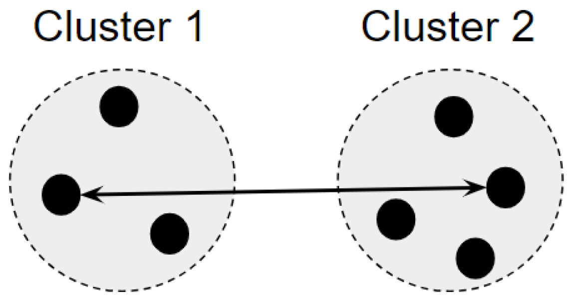
3.1. Agglomerative Clustering

The agglomerative clustering (AC) model is a popular unsupervised learning model used to group similar data into hierarchical clusters in a bottom-up clustering process. AC starts by considering each data point as an individual cluster and then iteratively combines the clusters closest to each other based on some distance metric until all the data points are in a single cluster or until a stopping criterion is met [44].

Thus, considering a dataset with N elements, where the i-th element is represented by a vector of characteristics $x_i$, the initial stage of agglomerative clustering, known as linkage, is used to link the points to form candidate clusters according to a given metric. Therefore, let $D(a,b)$ be the distance between clusters a and b.In each iteration, the pairs of clusters that were not previously joined are inspected, and the pair of clusters with the minimum value in D is joined to form a new cluster a. As a result, the distances $D(a,b)$ between the new cluster a and all the other clusters need to be recalculated. Thus, taking s and t as the pair of clusters that have been joined and defining $c\left[i\right]$ as the way to represent an object i in cluster c, the four linkage methods used in this paper [45] are the following:

• Single: The distance between clusters a and b is given by the smallest distance between every pair of objects (a[i], b[j]), according to Equation (1). Figure 1 illustrates this method.

  $$D(a,b)=\underset{ij}{min}\left\{D(a\left[i\right],b\left[j\right])\right\}$$

  (1)

  Figure 1. Representations of the single linkage method.

  Figure 1. Representations of the single linkage method.
• Average: Defines the new distance as the average distance between objects in a and b according to Equation (2), where $\left|c\right|$ represents the number of objects in cluster c. This method is illustrated in Figure 2.

  $$D(a,b)=\sum _{ij}{\displaystyle \frac{D\left(a\right[i],b[j\left]\right)}{\left|a\right|\left|b\right|}}$$

  (2)

  Figure 2. Representations of the average linkage method.

  Figure 2. Representations of the average linkage method.
• Complete: Calculates the largest distance between every pair of objects between clusters $a\left[i\right]$ and $b\left[j\right]$, according to Equation (3), and as illustrated in Figure 3.

  $$D(a,b)=\underset{ij}{max}\left\{D(a\left[i\right],b\left[j\right])\right\}$$

  (3)

  Figure 3. Representations of the complete linkage method.

  Figure 3. Representations of the complete linkage method.
• Ward: Joins clusters leading to the minimum increase in within-cluster variance. This can be performed by setting the distances as Equation (4), where $T=\left|v\right|+\left|s\right|+\left|t\right|$. Figure 4 illustrates this method.

  $$D(a,b)=\sqrt{{\displaystyle \frac{\left|b\right|+\left|s\right|}{T}}D{(b,s)}^2+{\displaystyle \frac{\left|b\right|+\left|t\right|}{T}}D{(b,t)}^2-{\displaystyle \frac{\left|b\right|}{T}}D{(s,t)}^2}$$

  (4)

  Figure 4. Representations of the ward linkage method.

  Figure 4. Representations of the ward linkage method.

3.2. Principal Component Analysis

Principal component analysis is a widely employed technique in machine learning to reduce the dimensionality of data without significant loss of information. Its objective is to transform correlated variables into a new uncorrelated set, known as principal components, while preserving the original variation of the dataset as much as possible [46]. These components are mathematically obtained through weighted linear combinations of the initial variables, with their coefficients determined by the eigenvectors of the correlation matrix and their variations associated with the corresponding eigenvalues. This approach aims to maximize the understanding of the variation in the data, requiring fewer components when there is a higher correlation among the original variables. The hierarchical structure of PCA enables the condensation of complex data into independent components, gradually revealing more specific aspects of the analysis [47].

In practical terms, the first step consists of calculating the covariance matrix ($\mathbf{C}$) from the data matrix (${\mathbf{X}}_{m\times n}$) according to Equation (5). Next, the decomposition of the covariance matrix into a set of orthogonal vectors (principal components) can be performed via the singular value decomposition (SVD) algorithm, as shown by Equation (6), where $\mathbf{\Lambda }$ contains the ranked eigenvalues of $\mathbf{C}$ and $\mathbf{V}$ is the orthogonal matrix containing their corresponding eigenvectors.

$$\mathbf{C}={\displaystyle \frac{1}{n-1}}\sum _{i=1}^n(x_i-\overline{x}){(x_i-\overline{x})}^T$$

(5)

$$\mathbf{C}=\mathbf{V}\mathbf{\Lambda }{\mathbf{V}}^T$$

(6)

Finally, it is possible to determine the number of principal components to be used to represent the original dataset without significant loss of information. As the eigenvalues provide information on the variance of the principal components, it is possible to estimate a relationship between the degree of information that will be preserved (I) and the number of principal components ($r<n$) used, as shown by Equation (7).

$$I={\displaystyle \frac{{\sum }_{i=1}^r{\Lambda }_i}{{\sum }_{j=1}^n{\Lambda }_j}}$$

(7)

3.3. Feature Selection Approach

The implemented algorithm assigns weights to the features based on criteria derived from box-plot statistics, guiding the decision process for selecting attributes at a later moment. Essentially, this algorithm classifies the features according to their distribution in the different predicted clusters based on box-plot statistics (quartiles, interquartile range, upper and lower limits of the distribution) and assigns relevance scores based on these comparisons. Finally, the features with the highest scores are considered to be the most discriminating among the clusters.

The estimation of the relevance of each of the features extracted from the signals was implemented in a simplified way, as described in Algorithm 1, and basically consists of two stages:

• Calculation of statistics by cluster and feature: For each grouping of each feature, the first (Q1) and third (Q3) quartiles, the interquartile range (iqr) is calculated. Then, the upper (UL) and lower (LL) limits of the distribution are estimated according to Equations (8) and (9):

  $$LL=Q1-1.5\ast (Q3-Q1)$$

  (8)

  $$UL=Q3+1.5\ast (Q3-Q1)$$

  (9)
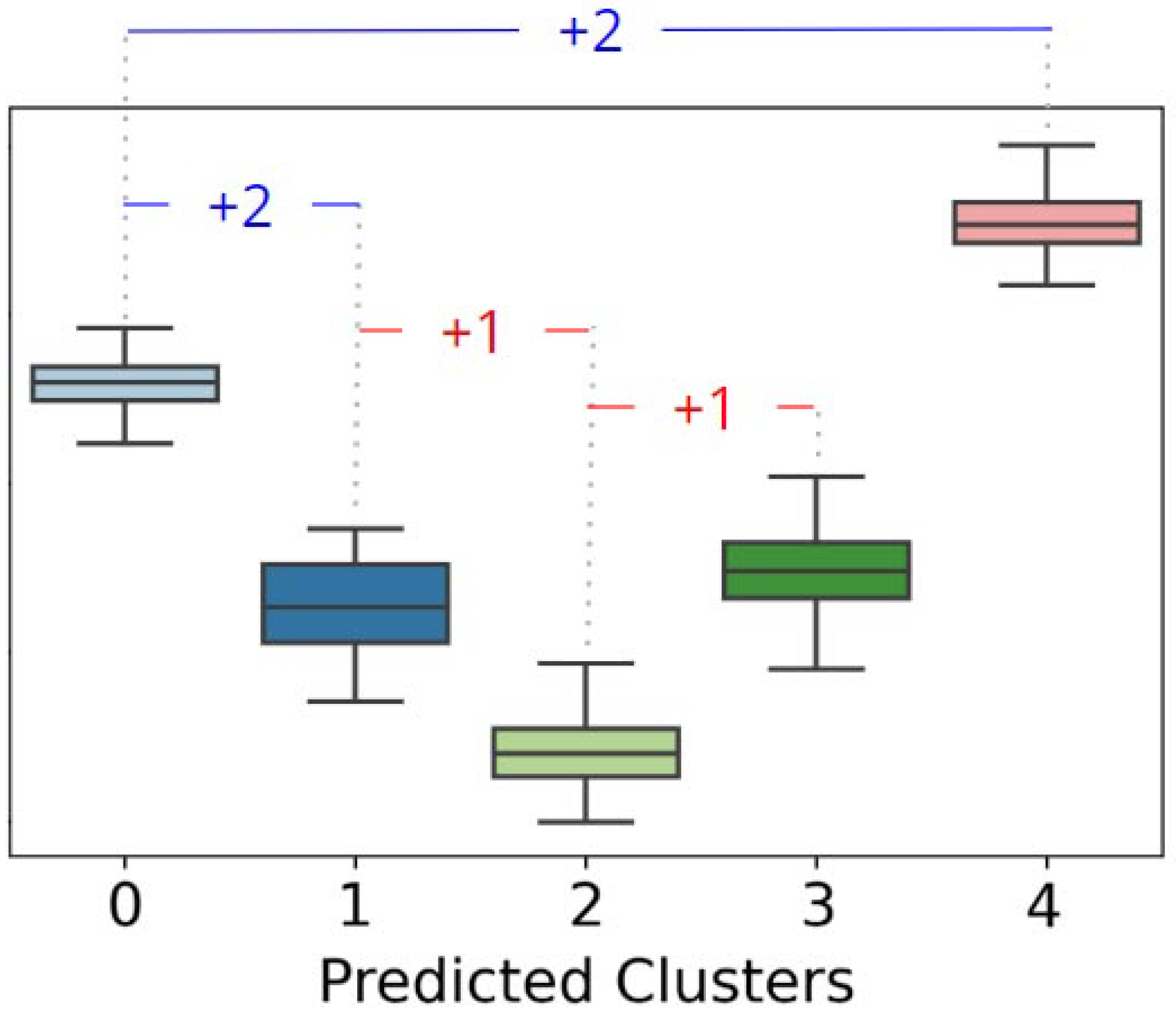
• Assigning scores: This stage begins by evaluating the interquartile ranges of all the clusters. The existence of at least one null interval invalidates the attribute for further scoring analyses. If there is no null iqr, the algorithm carries out a pairwise check of the clusters for a given feature, first comparing the lower limit of one cluster with the upper limit of the other and then the first quartile with the third quartile of the respective clusters. The first check consists of assessing whether the minimum value of the distribution of one cluster (reference) is greater than or equal to the maximum value of the distribution of the other cluster under analysis. If this is met, the algorithm bonuses the feature with 2 points and breaks the iteration, moving on to the next reference cluster. Otherwise, the second evaluation is carried out, checking whether the Q1 of the reference cluster is greater than the Q3 of the other cluster under analysis. In this case, the algorithm bonuses the feature with just 1 point and also breaks the repetition structure to continue analyzing the next reference cluster. In other cases where none of these behaviors are observed, there is no bonus for the feature.

Algorithm 1 Algorithm for assigning weights in the process of identifying the relevance of features.

1: for $feature$ in $\mathbf{X}$ do    2:      for $cluster$ in $N\_clusters$ do    3:    Calculates the first quartile (Q1)   4:    Calculates the third quartile (Q3)   5:    Calculates the interquartile range (iqr)   6:    Calculates the lower limit of the distribution (LL)   7:    Calculates the upper limit of the distribution (UL)   8:      end for    9: end for  10: for $feature$ in $\mathbf{X}$ do  11:      if any cluster has $iqr\left(feature\right)=0$ then  12:    Continue to the next iteration; 13:      else  14:    for $cluster\_i$ ← 0 to $N\_clusters-1$ do  15:      for $cluster\_j$ ← 0 to $N\_clusters$ do  16:        if $cluster\_i\ne cluster\_j$ then  17:          if $LL(cluster\_i,feature)\ge UL(cluster\_j,feature)$ then  18:           Increases feature weight by +2 points; 19:           Break; 20:          else if $Q1(cluster\_i,feature)>Q3(cluster\_j,feature)$ then  21:           Increases feature weight by +1 points; 22:           Break; 23:          end if  24:        else  25:          Continue to the next iteration; 26:        end if  27:      end for  28:    end for  29:      end if  30: end for

To illustrate the feature bonus scheme, Figure 5 shows the behavior of the 5 clusters of a given attribute so that the algorithm bonuses it with 6 points, considering only a single iteration of the ML model used. The first comparison takes place between clusters 0 (reference) and 1 so that the feature receives two bonus points, as the lower limit of cluster 0 is higher than the upper limit of cluster 1. This breaks the iteration, and cluster 1 becomes the reference for comparison. It is first compared with cluster 0, but the checks are not met. Subsequently, it is compared with cluster 2 in order to fulfill the second check (Q1 > Q3) and accumulate 1 more bonus point. The repetition structure is broken, and the evaluations are based on cluster 2 as a reference. In this case, comparisons are made with the other clusters, but none of the criteria are met. Thus, taking cluster 3 as a reference, the first comparison that meets any criteria is with cluster 2, as quartile 1 of the reference cluster is higher than quartile 3 of cluster 2. Finally, cluster 4 is analyzed so that the first comparison (with cluster 0) meets the criterion of the lower limit of the reference cluster (4) being higher than the upper limit of the other cluster under analysis (cluster 0). Thus, the feature accumulated 6 relevance points in a single run of the algorithm, with a further 24 evaluations to be carried out with other training sets and predicted labels.

3.4. Extrinsic Performance Metrics

Given the knowledge of the true class assignments of the samples, three extrinsic metrics were used to evaluate the clustering performance: homogeneity, completeness, V-measure, and adjusted Rand score.

The concepts of extrinsic metrics homogeneity, completeness, and V-measure were introduced by Rosenberg and Hirschberg [48]. In general, homogeneity evaluates if each cluster contains only members of a single class. Determining how close a proposed cluster is to its ideal is conducted by evaluating the conditional entropy of the class distribution based on the proposed clustering. Completeness, in turn, is symmetrical to homogeneity and evaluates if all members of a given class are assigned to the same cluster. The evaluation of the degree of distribution distortion of the clusters is calculated using the conditional entropy of the proposed cluster distribution given the true class of the data points. Finally, the V-measure is defined as an entropy-based metric that specifically assesses the success with which the homogeneity and integrity requirements were satisfied. In practice, the V-measure is calculated as the harmonic average of several homogeneity and integrity values.

The adjusted Rand score calculates a similarity measure between two clusterings by taking all pairs of samples and counting whether they are allocated to the same or different clusters in the expected and actual clustering. Thus, this measure has values near 0 for random labeling, regardless of the number of clusters or samples, and exactly 1 when the clusterings are equal (up to a permutation).

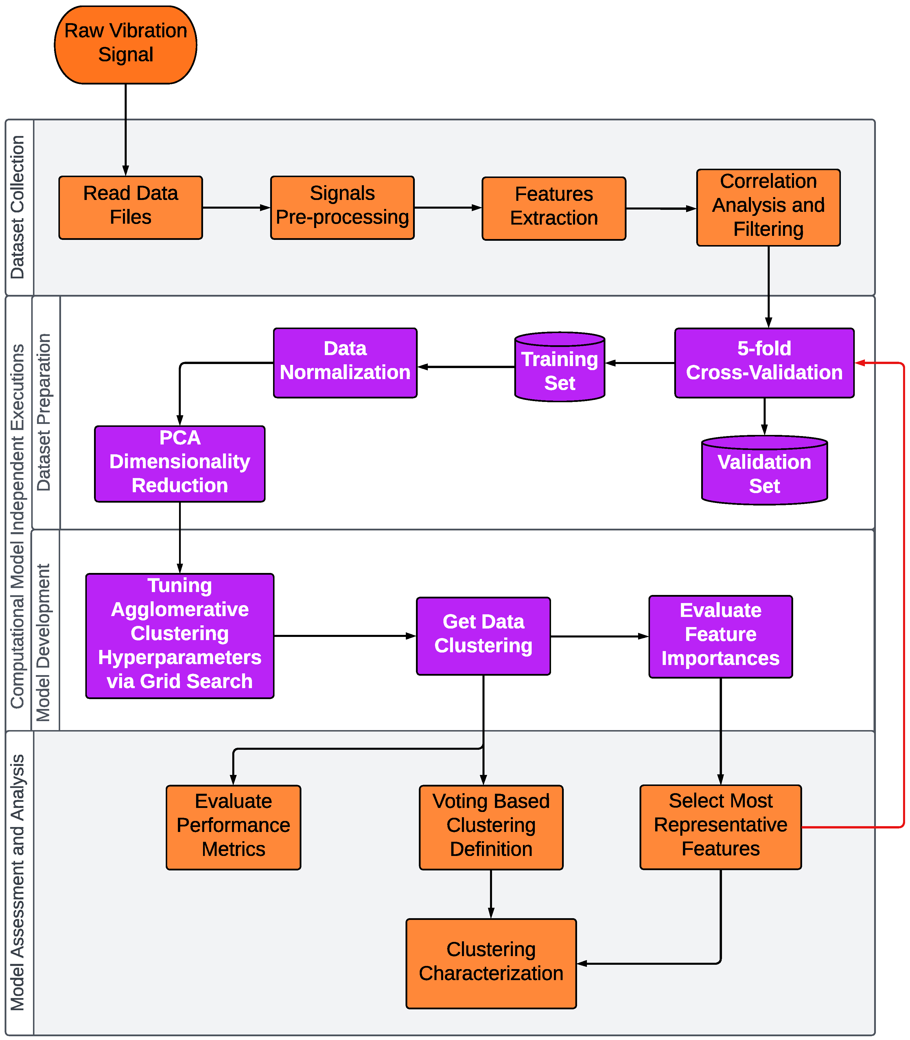
4. Proposed Approach

The proposed approach basically consists of six steps: (i) the reading and pre-processing of vibration signals; (ii) the feature extraction in three different domains; (iii) the application of a correlation filter, eliminating the highly correlated features; (iv) the execution of the unsupervised computational model; (v) feature selection based on those importance analyses; and, finally, (vi) extrinsic performance metrics evaluation and the clusters characterization defined by voting-based process. Figure 6 illustrates these steps in more detail.

First, the files containing the raw vibration signals of the structures are read, i.e., imported into Python—version 3.8.1, whose representation consists of a vector of real values of the amplitudes of the sampled signal. Each signal is then pre-processed. This process consists of properly partitioning the vibration signals once the data from each case study have their own particularities and are organized in a specific way. Then, a feature extraction process is implemented with the aid of the TSFEL (Time Series Feature Extraction Library) [49] and Scipy [50] libraries, obtaining a total of 44 characteristics from each signal. Of these, 18 are temporal features, described in

Table 1. Description of temporal features extracted from the signals.

Feature	Description
$X_1$	Absolute energy of the signal *.
$X_2$	Area under the signal curve computed with trapezoid rule *.
$X_3$	Autocorrelation of the signal *.
$X_4$	Centroid along the time axis *.
$X_5$	Entropy of the signal using the Shannon Entropy **
$X_6$	Mean absolute differences of the signal.
$X_7$	Mean of differences of the signal.
$X_8$	Median absolute differences of the signal.
$X_9$	Median of signal differences.
$X_{10}$	Number of negative turning points of the signal.
$X_{11}$	Number of peaks from a defined signal neighborhood.
$X_{12}$	Peak to peak distance *.
$X_{13}$	Number of positive signal turning points *.
$X_{14}$	Signal traveled distance *.
$X_{15}$	Slope of the signal *.
$X_{16}$	Sum of absolute differences of the signal *.
$X_{17}$	Total energy of the signal *.
$X_{18}$	Computes the zero-crossing rate of the signal *.

* Feature defined in reference [49]. ** Feature defined in references [49,51].

; 10 are statistical indicators, described in

Table 2. Description of statistical features extracted from the signals.

Feature	Description
$X_{19}$	Compute the interquartile range of the data along the specified axis **.
$X_{20}$	Computes crest-factor of the signal.
$X_{21}$	Computes kurtosis of the signal *.
$X_{22}$	Computes skewness of the signal *.
$X_{23}$	Computes the maximum value of the signal *.
$X_{24}$	Computes the minimum value of the signal *.
$X_{25}$	Computes root mean square of the signal *.
$X_{26}$	Computes mean value of the signal *.
$X_{27}$	Computes median of the signal *.
$X_{28}$	Computes standard deviation of the signal *.

* Feature defined in reference [49]. ** Feature defined in reference [50].

; and the last 16 are features from the spectral domain, described in

Table 3. Description of spectral features extracted from the signals.

Feature	Description
$X_{29}$	Barycenter of the spectrum *.
$X_{30}$	Represents the amount of decreasing of the spectra amplitude *.
$X_{31}$	Computes the signal spectral distance. Distance of the signal’s cumulative sum of the FFT elements to the respective linear regression *.
$X_{32}$	Computes the spectral entropy of the signal based on Fourier transform *.
$X_{33}$	Measures the flatness of a distribution around its mean value *.
$X_{34}$	Computes the number of positive turning points of the FFT magnitude signal *.
$X_{35}$	Computes the spectral roll-off of the signal. The spectral roll-off corresponds to the frequency where 95% of the signal magnitude is contained below this value *.
$X_{36}$	Computes the spectral roll-on of the signal. The spectral roll-on corresponds to the frequency where 5% of the signal magnitude is contained below this value *.
$X_{37}$	Measures the asymmetry of a distribution around its mean value *.
$X_{38}$	Computes the spectral slope. The spectral slope is computed by finding constants m and b of the function aFFT = mf + b, obtained by linear regression of the spectral amplitude *.
$X_{39}$	Measures the spread of the spectrum around its mean value *.
$X_{40}$	Computes the amount of variation of the spectrum along time. Spectral variation is computed from the normalized cross-correlation between two consecutive amplitude spectra *.
$X_{41}$	Computes maximum power spectrum density of the signal *.
$X_{42}$	Computes maximum frequency of the signal *.
$X_{43}$	Computes median frequency of the signal *.
$X_{44}$	Computes power spectrum density bandwidth of the signal. It corresponds to the width of the frequency band in which 95% of its power is located *.

* Feature defined in reference [49].

. After extracting all these features from each signal, a correlation analysis is carried out, eliminating highly absolute correlated features. Finally, after carrying out these procedures, the data are ready to be used as input for the machine learning model.

The computational model is run 5 times independently, considering the cross-validation procedure with 5 folds in each run. Thus, a total of 25 subsets are evaluated. In each of these subsets, the features are scaled to values between 0 and 1 (min–max scale) and then submitted to principal component analysis, which is used to reduce the dimensionality of the subset to 3 dimensions. After that, a grid search is carried out to optimize the hyperparameters of the agglomerative clustering model and estimate the number of clusters that best fit the data, basing the choices on the highest silhouette coefficient.

Table 4. Candidate values for internal parameters in the grid search process.

Parameters	Possible Values
Linkage	Ward, Complete, Average, Single
Metric	Euclidean, L1, L2, Manhattan, Cosine
Number of Clusters	[2, 3, 4, 5, 6, 7, 8]

shows the parameters evaluated in this optimization process.

By defining the best model parameters, it is possible to predict and group the data. As this is an adaptation of a supervised problem to an unsupervised approach, it is possible to use some extrinsic metrics to assess the model’s clustering performance. At the same time, for each subset considered, the features are evaluated in terms of their relevance, according to the feature selection approach previously described. At the end of the runs, the most important features are identified using a defined scoring threshold and are then selected to create a new subset of features. This subset, in turn, is evaluated by re-running the proposed process. Finally, after all the runs, a voting-based process is used to define the cluster for each sample, based on the definitions made throughout the runs. Thus, the characterization of the clusters is carried out based on the definition of the clusters and the most relevant features.

5. Computational Experiments

The computational experiments were conducted on a computer with the following specifications: Intel(R) Core(TM) i5-1135G7 CPU @ 2.40 GHz, 8 GB RAM, and Windows 10 Home as an operating system. Additionally, the codes were implemented in Python, based on pandas [52], NumPy [53], matplotlib [54], seaborn [55], tsfel [49], scikit-learn [56], and scipy [50] libraries.

As a way of evaluating the proposed approach, four case studies from different civil structures are considered. The first one consists of monitoring 5 load scenarios of a slender two-story aluminum frame. This structure was evaluated by Finotti et al. [57], which makes use of an unsupervised deep learning algorithm based on sparse autoencoders (SAEs) and the Shewhart T Control Chart ($T^2$) to identify structural changes in a slender frame. Then, the second and third case studies are based on the database provided by Sun [58], which presents a set of data to identify anomalies in walls made of different materials and another dataset whose purpose is to identify three severity degrees of damage to a wall. Finally, the last study case refers to the well-known Z24 bridge benchmark database, whose description is provided by Maeck and De Roeck [59].

5.1. Two-Story Slender Aluminum Frame

An aluminum frame made up of 6 bars measuring 300 mm long × 15.875 mm wide and 1.587 mm thick was built at the Images and Signals Laboratory (LIS) of the Federal University of Juiz de Fora. The structure was excited by the impact of a pendulum that collided with the structure in a certain position after coming to rest from a predetermined fixed height. Four piezoelectric accelerometers were used to measure the structural responses resulting from the impact. Figure 7 shows more details of the experimental scheme described, showing the positioning of the accelerometers ($Ac$) and the impact height of the pendulum.

To change the dynamic characteristics of the structure, two supports ($m_1$ and $m_2$) were installed on the horizontal bars, as shown in Figure 7, in order to simulate structures with different external loads. Therefore, masses of 7.81 g were gradually attached to the structure, which made it possible to consider 5 loading scenarios of the same structure as described below.

• Scenario 0: Structure in original condition. No additional mass is attached to the structure ($m_1=m_2=0$).
• Scenario 1: Only one additional 7.81 g mass is attached to the structure on the upper horizontal bar ($m_1$ = 7.81 g and $m_2=0$).
• Scenario 2: Two additional 7.81 g masses are attached to the structure on the upper horizontal bar ($m_1=$ 15.62 g and $m_2=0$).
• Scenario 3: Three additional 7.81 g masses are attached to the structure: two on the upper horizontal bar and one in the lower horizontal bar ($m_1$ = 15.62 g and $m_2=$ 7.81 g).
• Scenario 4: Four additional 7.81 g masses are attached to the structure: two on the upper horizontal bar and two in the lower horizontal bar ($m_1$ = 15.62 g and $m_2$ = 15.62 g).

The structural dynamic response recordings were collected by the four accelerometers at a sampling rate of 500 Hz for 8.192 s. Following the same protocol adopted by the reference paper [57], the reading process analyzed 200 files from each loading scenario. To minimize the transient portion of the signal coming from the impact on the structure, the initial 100 points (0.2 s) of each signal were discarded, considering only the next 500 points (1 s). After that, all 44 features were extracted from each signal, forming a dataset composed of 1000 samples (200 files × 5 loading scenarios) and 176 columns (44 features × 4 accelerometers). Then, the correlation filter was applied to this dataset matrix, eliminating 95 features whose correlation degree was greater or equal to 0.90 and leaving the dataset ready to feed the model.

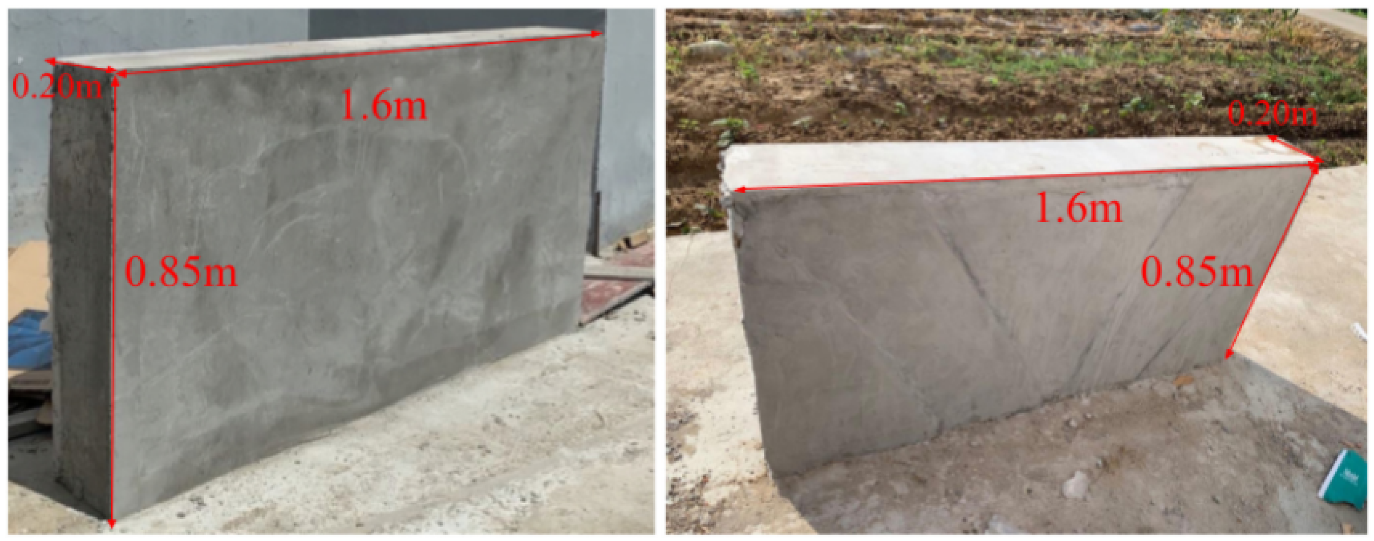
5.2. Wall Monitoring via Smartphone’s Vibration Response

To monitor the structural health of walls, Sun [58] proposed using a smartphone as an actuator and sensor, positioning it on the wall and letting it vibrate, while the device’s own accelerometer and gyroscope collected the dynamic responses.

Basically, two scenarios of data acquisition were considered. The first one, which composed our case study II—Section 5.2.1, consisted of obtaining dynamic responses from walls made of three different materials, with the sole aim of identifying whether there was damage or not. The second scenario consisted of identifying three severity degrees of damage in a specific wall built for this purpose. Case study III—Section 5.2.2, therefore, consists of evaluating our unsupervised approach from the database provided by this second scenario.

The dynamic tests were carried out 100 times on a healthy and on a damaged wall at 5 actuator vibration frequencies (10, 20, 30, 40, and 50 Hz), with a sampling frequency of 100 Hz. Only the z-axes of the acceleration signals were registered and considered in this paper.

5.2.1. Anomaly Detection

In order to differentiate between intact and damaged walls, the data acquired for this scenario consisted of dynamic tests on modern building walls made of three different materials, which were labeled as baker bricks, baker hall, and office wall. Thus, a total of 600 samples were generated, considering the 5 perspectives of excitation frequencies. Of these, 200 samples refer to each of the walls, so 100 identify an intact wall and the other 100 a damaged wall.

However, an analysis of the length of the signals revealed that some of the files presented a divergence in the size of their time series. It was, therefore, decided to standardize the length of the signals to 480 points in the pre-processing stage. As a consequence, the shorter signals (18 in total) were discarded while the larger signals were truncated. After that, those 44 features were extracted from each processed signal, considering the different excitation frequencies as one sample of vibration response. Thus, the final dataset was composed of 582 samples (600 original samples − 18 shorter signals discarded) and 220 columns (44 features × 5 excitation frequencies). Finally, the correlation filter was applied, aiming to eliminate those features with a correlation degree greater or equal to 0.90, leaving the final dataset composed of 121 columns and ready to feed the model.

The proposed model faced significant challenges in effectively grouping the data into the categories damage × no damage. Then, a second evaluation was conducted after including the wall materials as input variables for the model. However, the clustering performance still did not meet expectations. Considering that the physical vibration model incorporates the stiffness matrix of the wall material, as highlighted by [58], and that structural damage can affect its stiffness, the inferior performance of the clustering approach in these scenarios was somewhat expected. This is because the method might struggle to differentiate between cases, as similar vibration behavior can arise from walls made of different materials. To clarify, let us consider three materials: A, B, and C, where A has the highest stiffness, B is intermediate, and C has the lowest. If one of these materials, such as A, suffers damage, its stiffness would decrease. This damaged material A could then exhibit stiffness levels (and vibration responses) similar to materials B or even C, leading to potential misclassification by the model.

In this sense, a third evaluation was carried out, submitting the data for each wall separately to the model. Thus, the dimensions of the input dataset for each wall, without considering the material as a variable and after the correlation filter, now consist of 196 rows × 121 columns (Baker Bricks); 194 rows × 121 columns (Baker Hall); and 192 rows × 121 columns (Office Wall). The results achieved by this third approach are shown in the following Section 6.2.1.

5.2.2. Damage Severity Identification

Unlike the previous case (Section 5.2.1), this perspective aims to identify the severity of internal damage to a wall. To achieve this, the authors built a brick wall with dimensions of 1.6 m × 0.85 m × 0.20 m, as shown in Figure 8, which made it possible to reproduce a scenario of a damaged wall with cracks of different depths: 2 mm, 4 mm, and 6 mm. In addition, a total of 100 samples were generated for the case without damage and, for the other cases, 50 samples for each type of damage, totaling 250 samples, each containing the dynamic responses resulting from the 5 excitation frequencies.

It is worth noting that in this case, a similar analysis of the lengths of the signals was conducted. However, the files had similar lengths, around 608 points, with the particularity that they all consisted of 600 or more points (≥6 s). In this way, no file was discarded during the pre-processing stage, which was only responsible for truncating the signals of greater length than the standard 600 points adopted. After that, all 44 features were extracted from each signal, and, by combining the different excitation frequencies for the same sample, the feature matrix then had 250 rows (3 different severity damage levels × 50 dynamic tests + 100 undamaged condition tests) and 220 columns (44 features × 5 excitation frequencies). Finally, the correlation filter was applied to eliminate the features with a correlation degree greater than or equal to 0.90, leaving the final dataset composed of 88 columns and ready to feed the model.

5.3. Z24 Bridge Benchmark

The Z24 was a highway in Bern, Switzerland, linking the communities of Koppigen and Utzenstorf, passing over the A1, which connects Bern to Zurich. The Z24 was a conventional two-cell post-tensioned concrete box girder bridge with a main span of 30 m and two side spans of 14 m, as shown by Figure 9. The bridge was built in 1963, but at the end of 1998, it had to be demolished to make way for a new railway, which required a longer side span.

However, with the proposal for the evaluation of the structural condition based on dynamic monitoring, a series of progressive damage tests were carried out before demolition. To perform this, it was necessary to install a series of sensors throughout the bridge structure, arranged as shown in Figure 10. It is also important to note that the measurements consisted of a complete test of both ambient vibration (AVT) and forced vibration (FVT), the latter carried out with the help of two shakers placed in the center span (SH2) on the Koppigen side span (SH1), as is also illustrated in Figure 10.

Among the different damage cases, we decided to consider only the scenarios of progressive lowering of the pier under the forced vibration test, consisting of 5 severity levels (20 mm, 40 mm, 80 mm, and 95 mm). However, according to Roeck et al. [60], the 20 mm lowering of the Koppigen pier appears to have no noticeable effect on the eigenfrequencies, while an increase in lowering (40 mm, 80 mm, and 95 mm) has a significant influence. Thus, we opted in this paper to consider only the last 3 lowering levels (40 mm, 80 mm, and 95 mm) and the undamaged condition, used as a reference measurement, totaling 4 damage scenarios.

According to the documentations provided with the database, the structural dynamic responses were collected in 9 setups with a sampling rate of 100 Hz. Each setup was composed of 8 segments of approximately 8192 points. As a consequence, a total of 288 dynamic responses (9 setups × 8 segments/setup × 4 monitoring scenarios) were used for the evaluations in this work. Moreover, we chose to consider only the reference sensors: R1 (only vertical vibration measurement), R2 (3 dimensions vibration measurement), and R3 (only vertical vibration measurement). After that, each segmented signal was then subjected to the feature extraction process to obtain those 44 features. As a result, a total of 220 columns (44 features × 5 dynamic responses from the sensors) were obtained from each vibration signal. Then, after the application of the correlation filter to eliminate features correlation degrees greater or equal to 0.90, the dataset consisted of 93 columns.

6. Analysis of the Results

This section aims to show the results achieved by applying the computational method to the four case studies described in Section 5, as well as characterizing the predicted clusters.

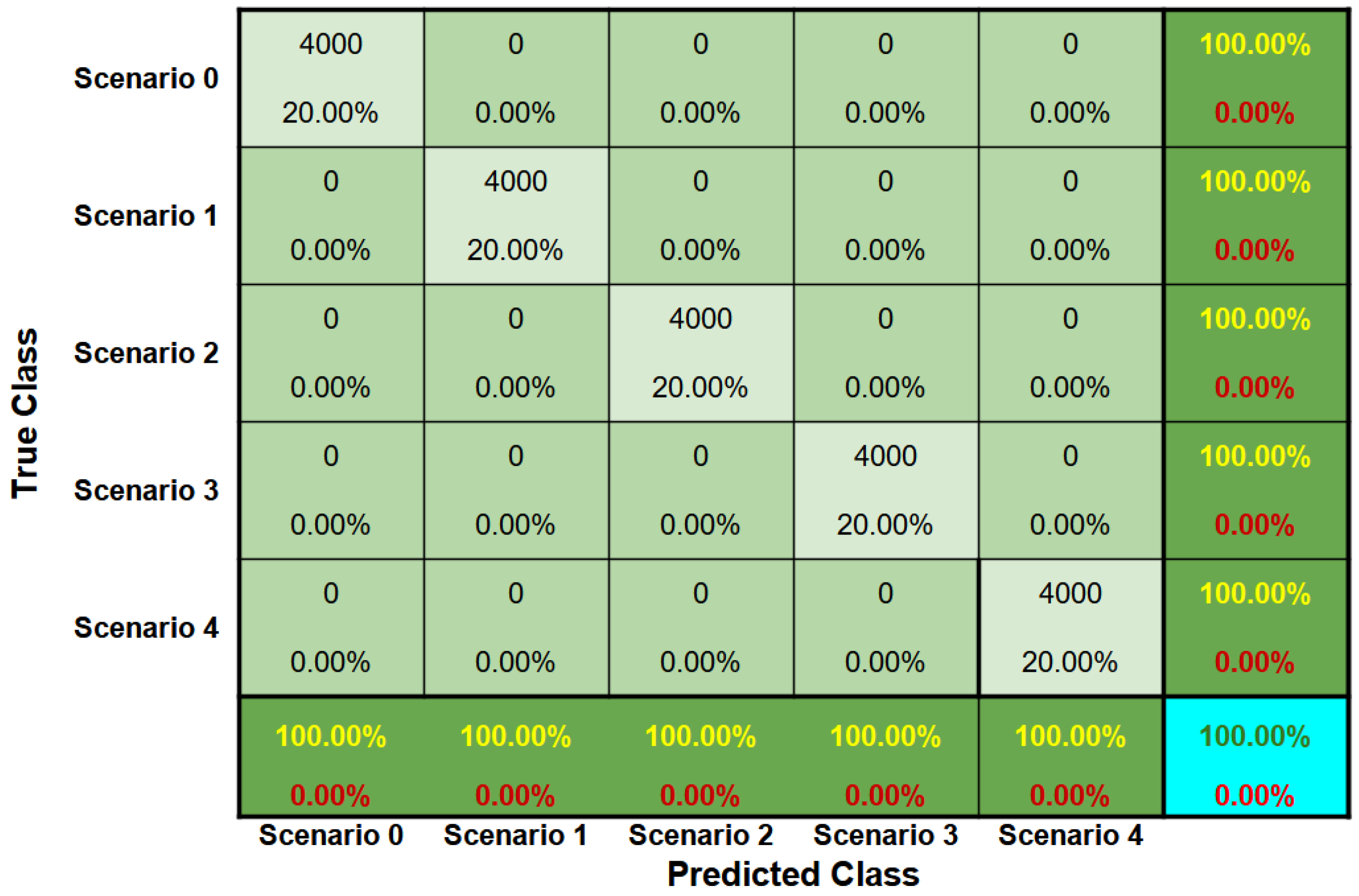
6.1. Two-Story Slender Aluminum Frame

Figure 11 reveals that by selecting just 12 features it is possible to achieve the same level of performance in this clustering task, as observed from the average results achieved shown in

Table 5. Average extrinsic performance metrics and their standard deviations referring to the 25 executions before and after the feature selection.

Performance Metric	Before Feature Selection	After Feature Selection
Homogeneity	1.0 (0.0)	1.0 (0.0)
Completeness	1.0 (0.0)	1.0 (0.0)
Adjusted Rand score	1.0 (0.0)	1.0 (0.0)
V-measure	1.0 (0.0)	1.0 (0.0)

.

From the results presented, no major difficulties were observed in detecting anomalies and the severity of the damage, probably because the vibration signals were collected in a controlled manner in the laboratory, with a very high signal-to-noise ratio. In addition, a parametric analysis revealed unanimity in the choice of parameters during the grid search process, resulting in linkage = ward, metric = euclidean, and n_clusters = 5.

A confusion matrix accumulated by the 25 iterations of the model was constructed, as illustrated by Figure 12. In addition, another confusion matrix was also obtained after a voting-based decision process. However, for this case, the confusion matrix remained the same, correctly grouping all the instances.

The process involved identifying relevant features by applying a threshold of 0.75, which led to the selection of 12 features across signals from the 4 accelerometers. When the methodological process was repeated with these selected features, the results remained comparable to those obtained with the full dataset. However, the modeling was computationally less expensive due to the reduced number of attributes (12 selected features compared to the original 81).

More specifically, when considering the signals from accelerometer 1, the process identified the following features as the most relevant: Centroid, Skewness, Spectral Entropy and Maximum Power Spectrum. The box-plots of those features are shown in Figure 13, and by looking at these plots, it can be seen that some clusters and behaviors stand out:

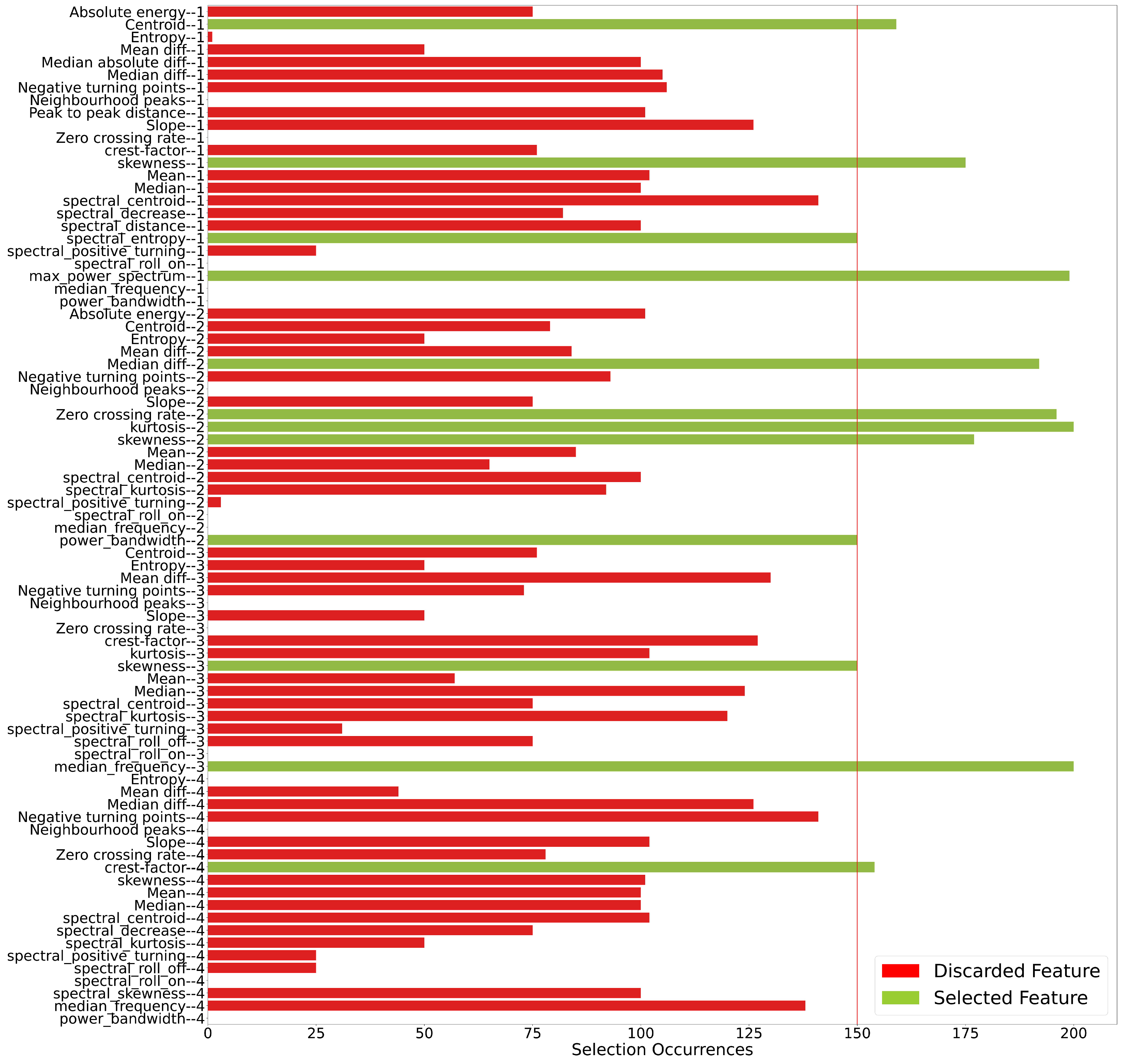
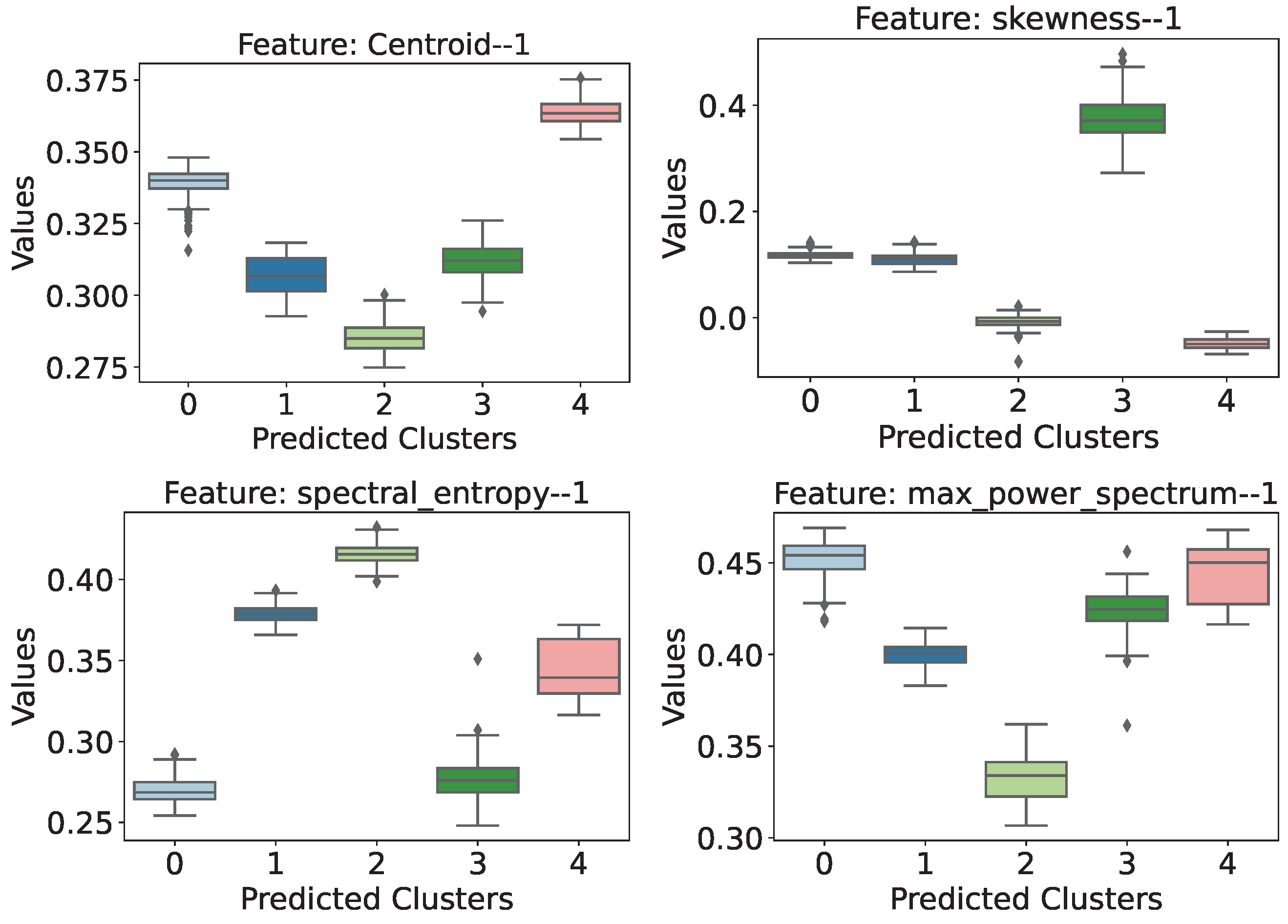
• Centroid: This attribute showed that the structure with the highest load (cluster 4) is associated with higher temporal centroid values and stands out because there is no interval overlap with the other cases.
• Skewness: The same behavior is identified in this attribute, with the difference that the highlight is cluster 3 ($m_1$ = 15.62 g and $m_2$ = 7.81 g) and with an even greater difference between the intervals.
• Spectral Entropy: In this case, it is possible to identify that there is a difference in the behavior of the attribute for the cases of a structure with loading. At first, this attribute could be useful in trying to localize the loading on the structure, as the introduction of weights in the upper portion of the frame (scenarios 1 and 2) have higher values and distributions than scenarios 3 and 4, which have both top and bottom loading. The addition of a mass, both from case 1 to 2 and from scenario 3 to 4, causes an increase in the entropy value of the signal power spectrum.
• Maximum Power Spectrum: Scenario 2 ($m_1$ = 15.62 g and $m_2$ = 0) is the cluster that stands out the most in this attribute, showing the lowest distribution of values.

For accelerometer 2, five more features were identified as relevant, as shown in Figure 14. These are Median of signal differences, Zero Crossing Rate, Kurtosis, Skewness, and Power bandwidth.

Thus, when evaluating the distribution of the selected features referring to accelerometer 2, some points are also worth highlighting:

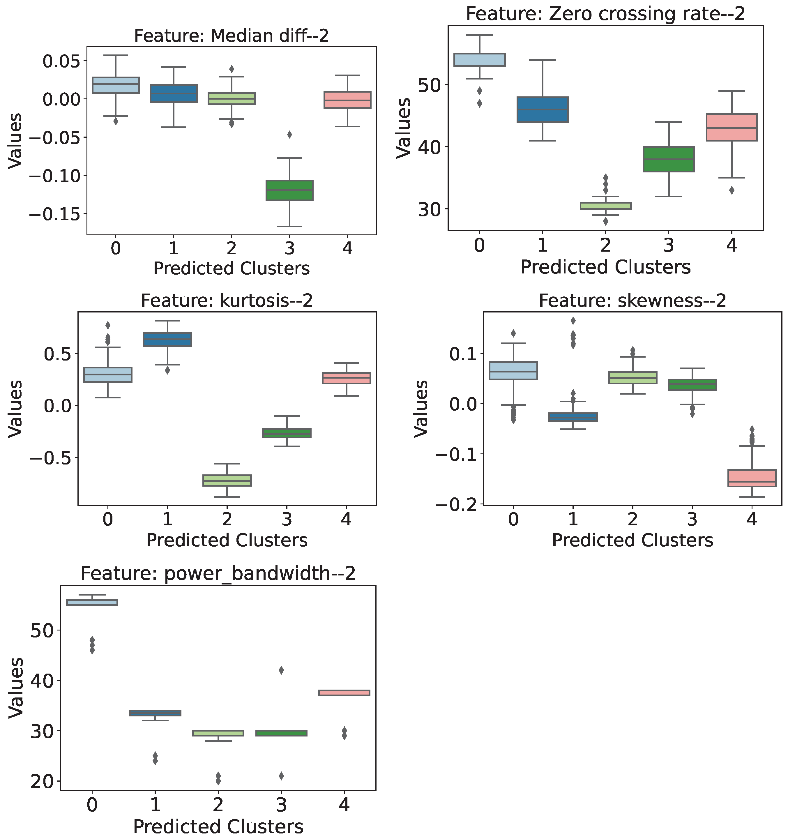
• Median of Signal Differences: In this attribute, it can be seen that cluster 3 stands out from the others, with the lowest values and no overlapping intervals.
• Zero Crossing Rate: Scenario 1 does not seem to be as well identified as a structure subject to external loading. On the other hand, when looking at scenarios 2, 3, and 4, there is a tendency for the value of the attribute to increase as the external load on the structure increases.
• Kurtosis: This feature shows that scenarios 2 and 3 do not overlap with any other grouping. It can also be seen that both scenarios have negative kurtosis values, which is more intense for scenario 2.
• Skewness: Cluster 4 stands out among the others, with the lowest skewness values, which are always negative.
• Power Bandwidth: This attribute is particularly noteworthy, as it seems to identify and represent a clear difference in behavior between an unloaded and loaded structure at any level. Even when taking into account the distribution’s outliers, it can be seen that a bandwidth above approximately 44 units identifies the structure as unloaded, while values below this threshold classify it as a structure subject to external loading.

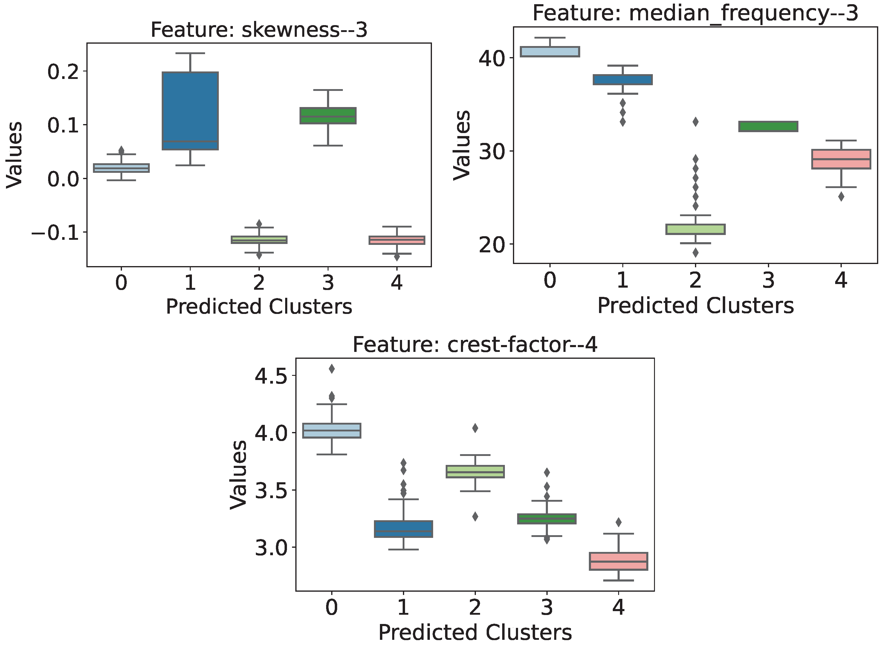
For accelerometers 3 and 4, only two and one attribute were identified for each of them, respectively. Skewness and Median Frequency were the most important features for accelerometer 3, and and Crest factor was the most relevant for accelerometer 4. The distribution of the values of these attributes is shown in Figure 15.

Due to the symmetry in the positioning of the accelerometers in the structure, the relevant attributes relating to accelerometers 3 and 4 present some more subtle highlights, but complement the attributes previously discussed.

• Skewness ($A{c}_3$): It can be seen in this case that the unloaded structure has a distribution of values very close to zero, while scenarios 1 and 3 have exclusively positive skewness values, in contrast to scenarios 2 and 4, whose values were strictly negative.
• Median Frequency ($A{c}_3$): In this feature, the unloaded structure showed the highest distribution of values and no overlapping of ranges among the other scenarios.
• Crest Factor ($A{c}_4$): Even though the intervals overlap, this seems to be an attribute that helps identify the unloaded scenario from the cases in which the structure is loaded. In general, the unloaded structure showed higher wave crest factor values, so the addition of external loads caused the crest factor values to drop.

6.2. Wall Monitoring via Smartphone’s Vibration Response

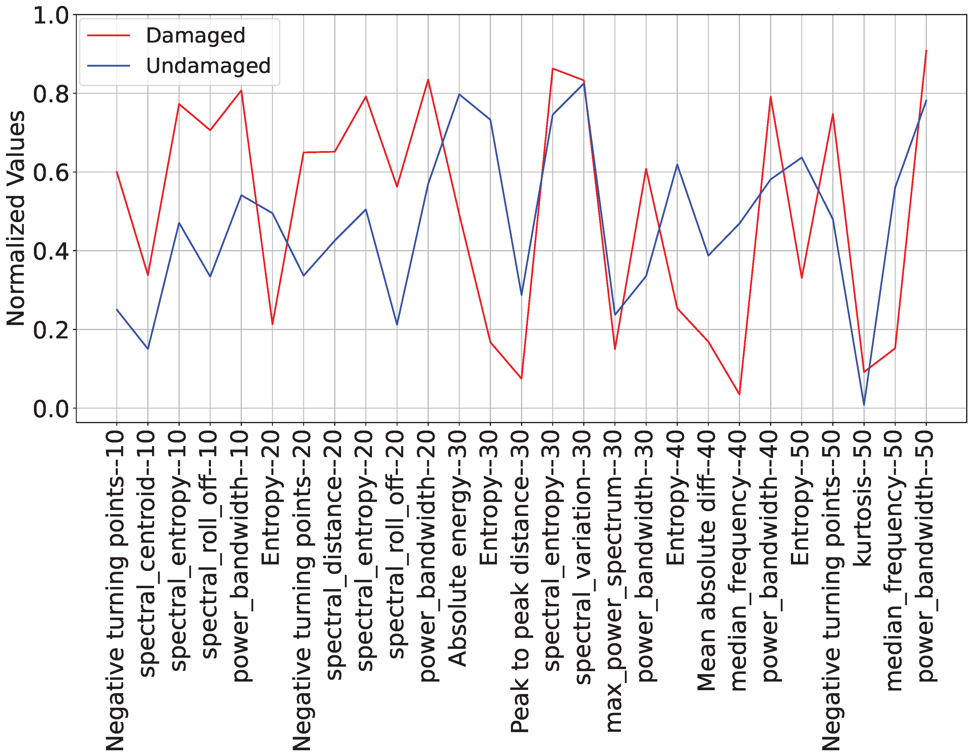
6.2.1. Anomaly Detection

The results achieved by the third clustering approach, i.e., considering each wall separately, are shown in

Table 6. Average extrinsic performance metrics and their standard deviations referring to the 25 executions, considering each wall separately without the feature selection.

Performance Metric	Baker Bricks	Baker Hall	Office Wall
Homogeneity	0.9921 (0.018)	0.8529 (0.0415)	0.9762 (0.0439)
Completeness	0.9921 (0.0182)	0.6139 (0.0342)	0.9765 (0.0432)
Adjusted Rand score	0.9959 (0.0094)	0.7302 (0.0375)	0.9855 (0.0283)
V-measure	0.9921 (0.0181)	0.7137 (0.0354)	0.9764 (0.0435)

and reveal a considerable improvement in unsupervised damage recognition performance.

Even so, by considering the process of selecting the most relevant features, it was possible to increase the average clustering performance, as shown by

Table 7. Averages of the extrinsic performance metrics and their standard deviations referring to the 25 executions, considering all data with feature selection.

Performance Metric	Baker Bricks	Baker Hall	Office Wall
Homogeneity	1.0 (0.0)	1.0 (0.0)	1.0 (0.0)
Completeness	1.0 (0.0)	1.0 (0.0)	1.0 (0.0)
Adjusted Rand score	1.0 (0.0)	1.0 (0.0)	1.0 (0.0)
V-measure	1.0 (0.0)	1.0 (0.0)	1.0 (0.0)

, as well as to reduce the size of the features sets to 4, 3, and 27 columns, respectively, to Baker Bricks, Baker Hall, and Office Wall cases. It is worth highlighting that to achieve these dimensions, we used a selection threshold defined as 80% of the maximum score for the Baker Bricks and Baker Hall cases and a threshold of 70% for the Office Wall scenario.

For each material scenario, an accumulated confusion matrix was constructed, as shown by Figure 16a, Figure 17a and Figure 18a. In addition, another confusion matrix was also obtained after a voting-based decision process, as illustrated by Figure 16b, Figure 17b and Figure 18b. After the voting-based decision on the groupings, all the instances were correctly predicted in the groupings in all three cases.

First, considering the Baker Bricks, the process of identifying the relevance of the features suggested the selection of 4 from 121 features. Specifically, we selected the Minimum Value for exciter signals with a frequency of 10 Hz, Peak to Peak Distance referring to the signals obtained by excitation frequency of 30 Hz, and Absolute Energy and Entropy with respect to the signals obtained at an excitation frequency of 40 Hz. The distribution of those features for each predicted cluster is shown in Figure 19. It can be seen that in all these features, there is practically no overlapping of intervals, except for the outliers present. Furthermore, the greatest difference between the intervals appears to be for the Minimum features, where the anomalous behavior of the wall is characterized by higher values, and the Absolute Energy attribute, where the values for the damaged structure are lower. This latter behavior is also observed for the other attributes: Peak to Peak Distance and Entropy.

In the context of Baker Hall walls, only the Absolute Energy extract from signals excited by a 10 and 20 Hz vibration frequency was selected. Their distributions are shown in Figure 20. It can be seen that the behavior of the attributes is similar so that the structure without damage has a lower absolute energy than the wall with damage. Furthermore, looking at the distributions, it seems that the excitation frequency that perhaps best describes this behavior is 10 Hz, as the overlap of the intervals was the smallest among the three cases.

Finally, considering the Office Wall scenario, a larger number of features was selected. Specifically, of the 27 attributes selected, 5 are associated with the excitation frequency of 10 Hz, 6 with 20 Hz, 7 with 30 Hz, 4 with 40 Hz, and, finally, 5 of them are associated with the excitation frequency of 50 Hz. Therefore, as this is a relatively larger number of attributes than in the previous cases, we decided to first evaluate the features using the averages of the normalized attributes. Figure 21 shows the graph with the average behavior of each attribute.

When analyzing the behavior of the distribution averages, it is possible to notice certain behaviors. Because they are average values, these behaviors can differ from the statistical ones, just like the box-plot. However, this type of analysis can also provide us with very relevant information about groupings, as follows:

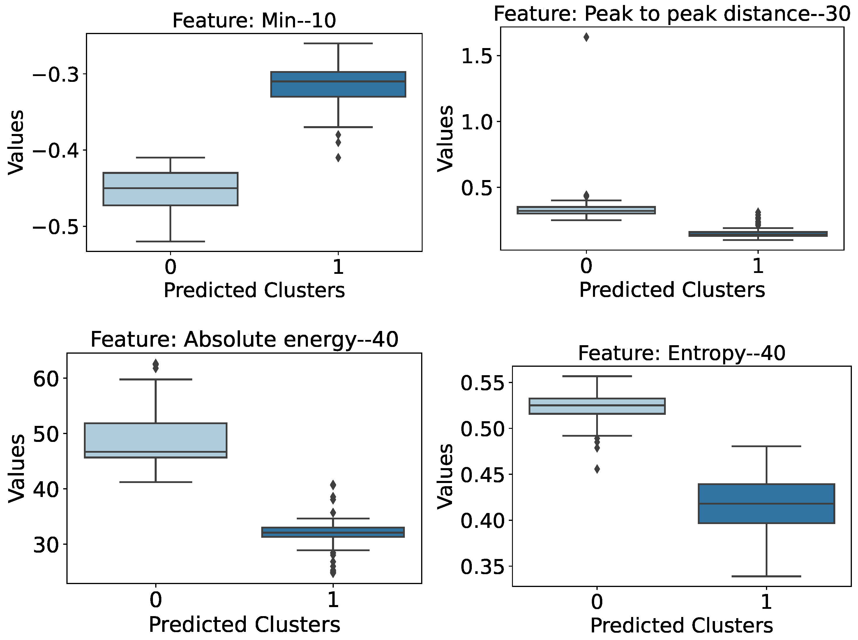
• Entropy (30 and 40 Hz): They show a difference of 56.5% and 36.5%, respectively, between the average values of the different wall conditions. In addition, the damaged cases have lower entropy values than the case of the wall in intact condition.
• Median Frequency (40 and 50 Hz): They show a difference of over 40.8% between the average values of the different wall conditions. Also, the damaged cases have lower values than the case of the wall in intact condition, as was expected, as, according to [61], damaged structures tend to have a lower natural frequency.
• Spectral Roll-Off (10 and 20 Hz): They show a difference of over 35.0% between the average values of the different wall conditions.
• Negative Turning Points (10 and 20 Hz): They show a difference of over 31.3% between the average values of the different wall conditions.

In addition, Figure 21 shows that at lower frequencies (10 and 20 Hz), the difference between the average behavior of the attributes is clearer. It can even be seen that in 10 of the 11 attributes selected at these frequencies, the case with the damaged wall has higher values than the case with the intact structure. From 30 Hz onward, the general behavior of the attributes starts to become less organized. However, from this frequency range onward, the greatest differences between the averages were observed, as in the case of Entropy (30 Hz)—56.5%—and the frequency medians (40 and 50 Hz)—43.4% and 40.8%, respectively.

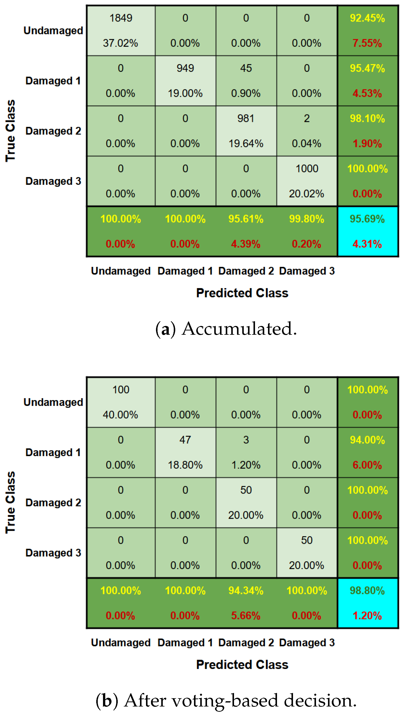
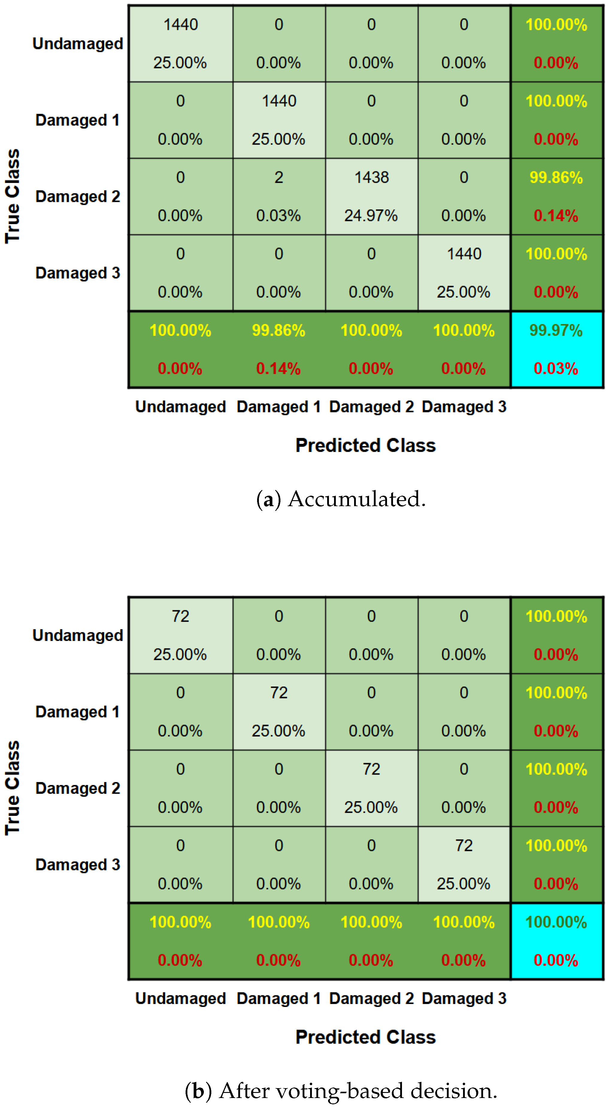
6.2.2. Damage Severity Identification

The feature importance analysis suggested selecting 3 of the 88 features using a threshold of 90% of the maximum score, culminating in an improvement in the performance of the clustering task, as apprehended from the results shown in

Table 8. Averages of the extrinsic performance metrics and their standard deviations referring to the 25 executions before and after the feature selection.

Performance Metric	Before Feature Selection	After Feature Selection
Homogeneity	0.9111 (0.0326)	0.9686 (0.0104)
Completeness	0.7052 (0.0248)	0.9171 (0.0657)
Adjusted Rand score	0.7413 (0.0314)	0.9251 (0.0680)
V-measure	0.7949 (0.0259)	0.9410 (0.0363)

.

Finally, after predicting the clustering of each instance, based on the frequency with which they were clustered throughout the independent runs and cross-validations, it is possible to take the values of the extrinsic metrics and obtain an overall picture of the clustering task. Thus, the following values were obtained: $Homogeneity=0.9654$, $Completeness=0.9659$, $AdjustedRandScore=0.9767$, and $V-Measure=0.9656$.

The confusion matrix for this case was also obtained both before (accumulated—Figure 22a) and after the voting-based decision of the clusters (Figure 22b). However, unlike the previous cases, it was not possible to obtain a correct prediction for all the instances. As depicted in Figure 22, the voting-based decision process led to an improvement in the model’s performance, so that only three instances had their classes wrongly predicted, classifying signals from a wall with type 1 damage as type 2 damage.

The cluster characterization stage was based on those three selected features and the predicted clusters after the definition carried out by the voting-based process. Thus, the behavior observed for each cluster and each selected feature is shown in Figure 23. It is possible to note, in these box-plots, that the absolute energy collected from the 10 Hz excitation vibration pattern aids the damage identification task, as there is a large difference in the distributions of the intact wall and the damaged ones. In general, healthy walls have a considerably lower absolute energy value than damaged walls. In addition, by evaluating the spectral centroid and the spectral decrease, it is possible to note that as the damage increases, the lower the values of those features are. In this sense, the healthy walls tend to present the highest values of spectral centroid and spectral decrease.

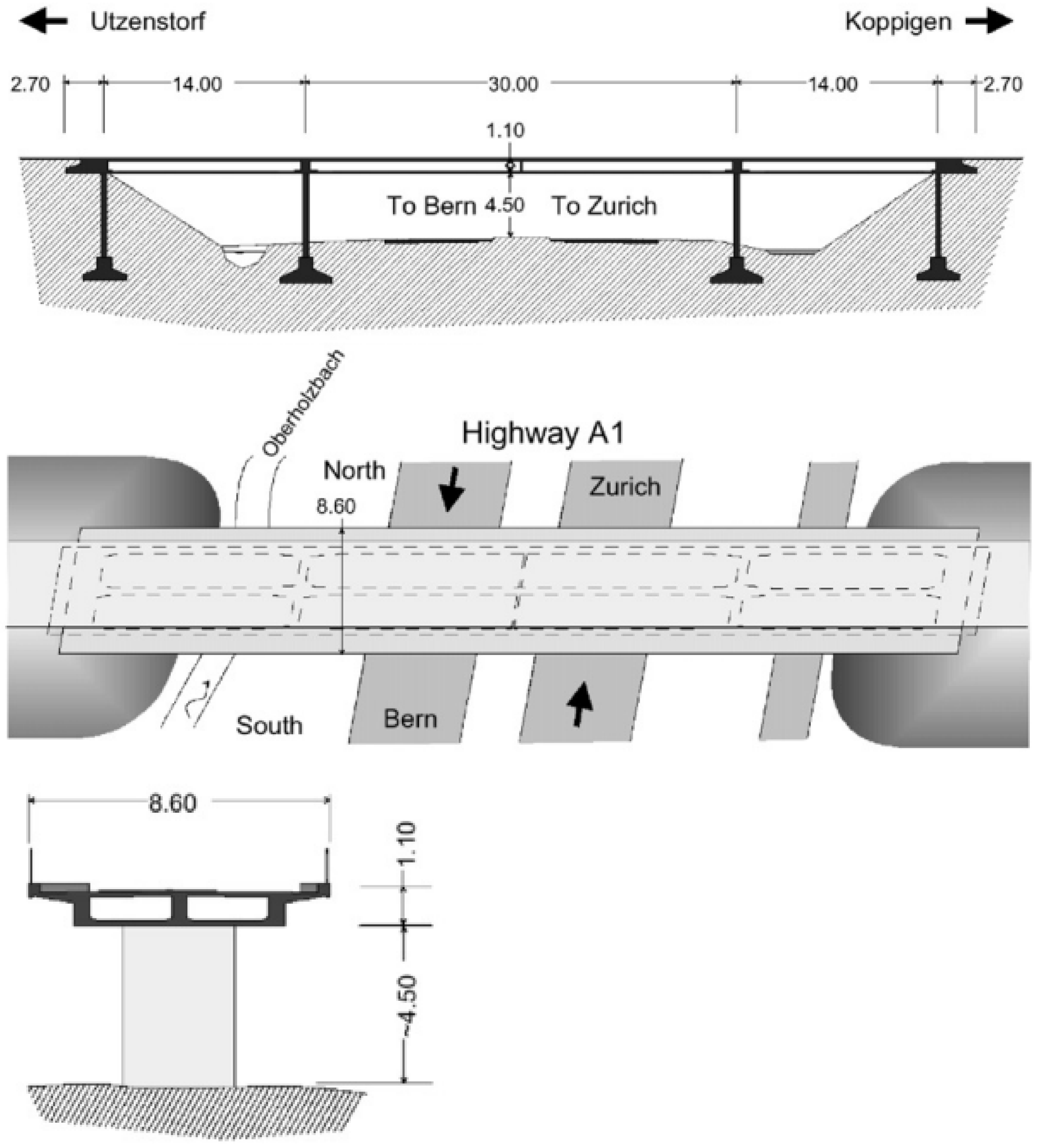
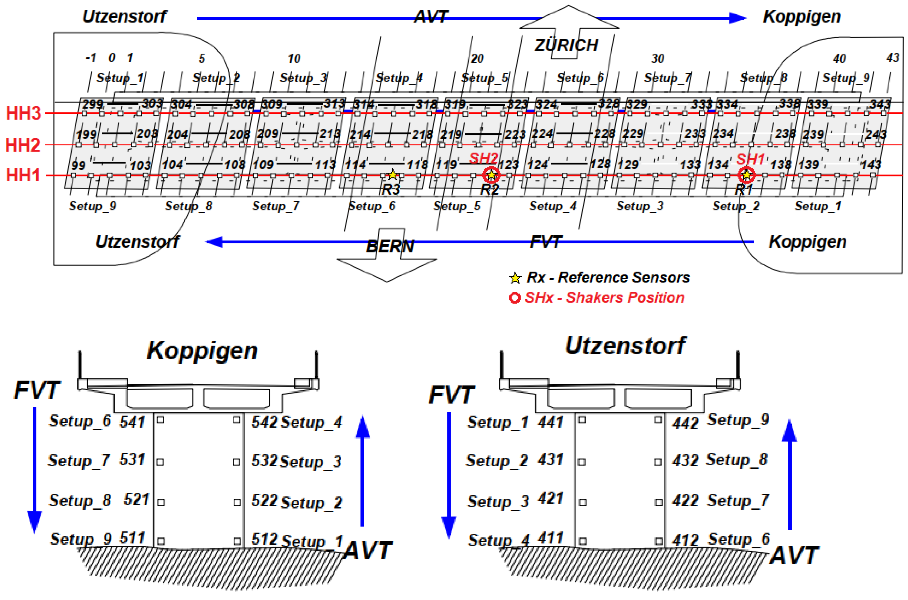
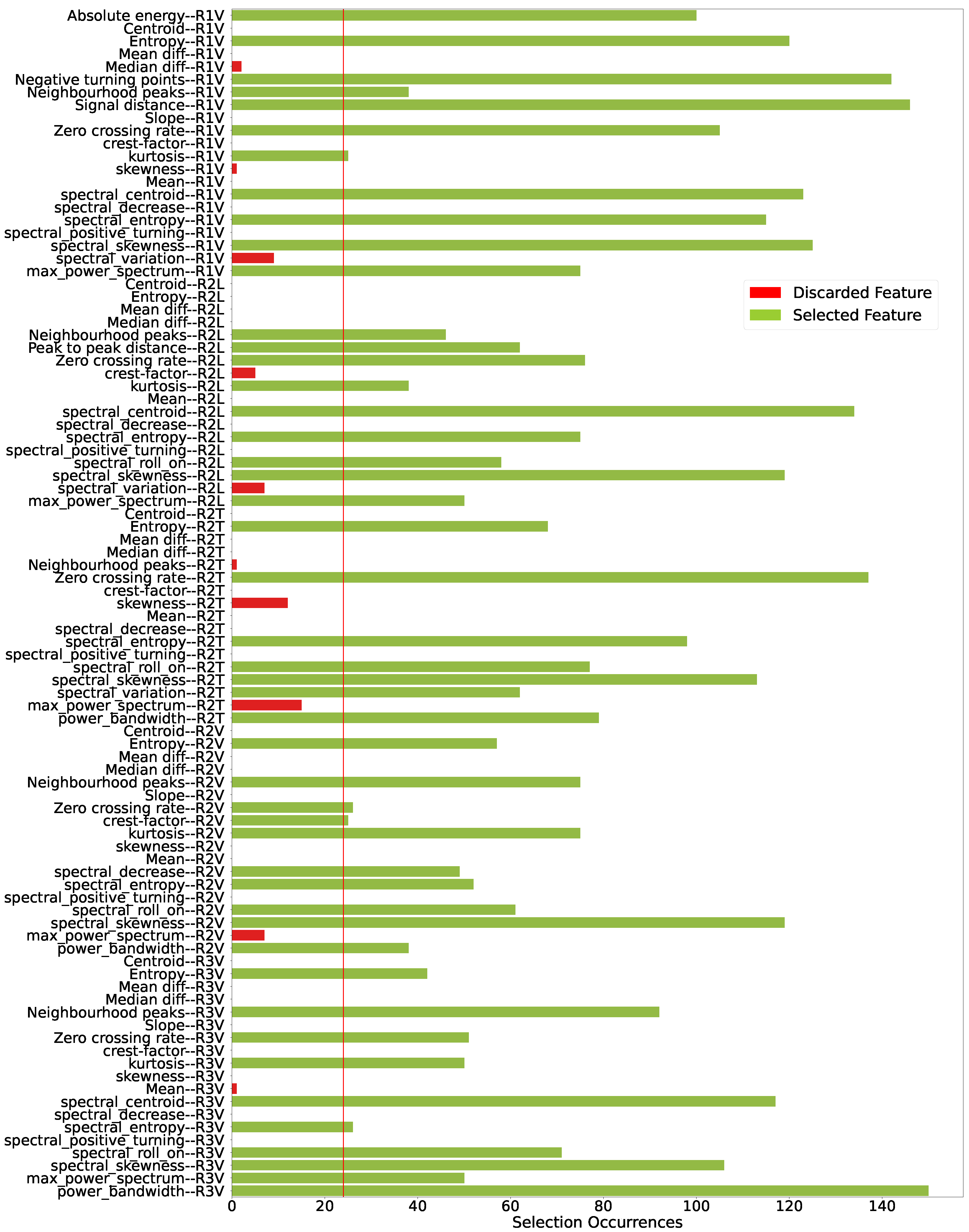
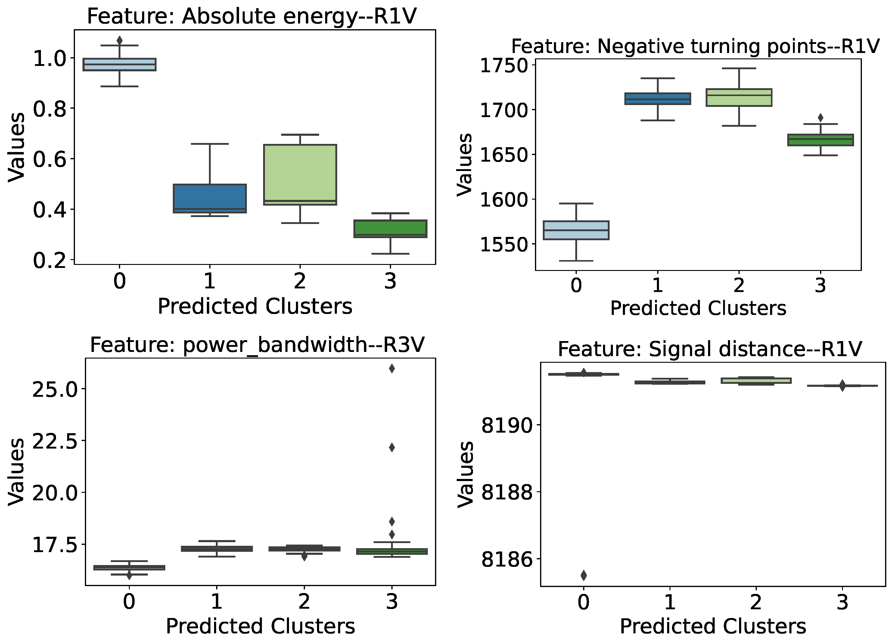
6.3. Z24 Bridge Benchmark

When analyzing the relevance of the features, it can be seen that, by defining a selection threshold of 16% of the maximum score, selecting 47 of the 94 features—Figure 24—is enough to achieve the same level of clustering performance for the model as shown by

Table 9. Average extrinsic performance metrics and their standard deviations referring to the 25 executions, considering the reference sensor in the forced vibration tests condition.

Performance Metric	Before Feature Selection	After Feature Selection
Homogeneity	0.9925 (0.0087)	0.9987 (0.0043)
Completeness	0.9926 (0.0086)	0.9987 (0.0043)
Adjusted Rand score	0.9944 (0.0066)	0.9991 (0.0031)
V-measure	0.9926 (0.0087)	0.9987 (0.0043)

.

Finally, after predicting the grouping of each instance using the voting-based procedure, it was possible to obtain the values of the extrinsic metrics and get an overview of this grouping task. This resulted in $Homogeneity=1.0$, $Competence=1.0$, $AdjustedRandScore=1.0$, and $V-Measure=1.0$. The excellence of the prediction in this case can also be seen in the confusion matrices illustrated by Figure 25a,b.

The cluster characterization stage was based on the 47 selected features and the definition of the clusters predicted by the voting-based process. After a preliminary analysis of the selected features, it was found that some of them show interesting distribution behaviors that are worth highlighting. Therefore, of the 47 attributes selected, only 12 are presented in this section.

Figure 26 and Figure 27 illustrate the behavior of the distribution of the most prominent features observed during the preliminary analysis. Figure 28, in turn, shows the distribution of the characteristics of the signals that have a second level of prominence, but which provide interesting insights.

Evaluating the attributes showed in Figure 26, the following behaviors can be highlighted:

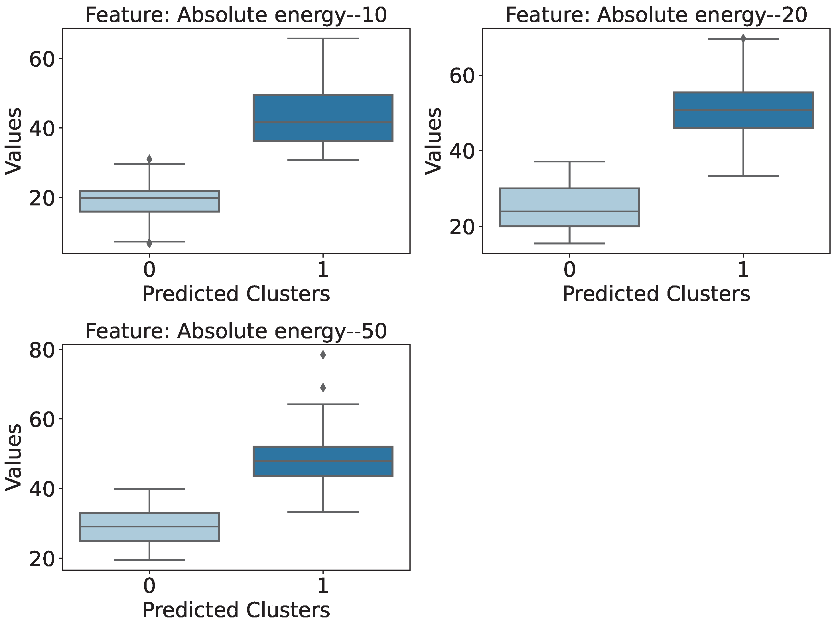
• Absolute Energy (R1 Sensor): This feature indicates that there is a distinction between the damaged and intact bridge scenarios. Higher absolute energy values tend to be associated with a healthy structure, while lower values of this attribute refer to one of the cases of lower damage assessed.
• Negative turning points (R1 Sensor): As with absolute energy, this characteristic extracted from the signals also appears to indicate healthy or damaged conditions. However, the behavior of this attribute is the opposite: lower values are associated with undamaged conditions, while higher values indicate the presence of one of the damages assessed.
• Power Bandwidth (R3 Sensor): This is yet another case where it is possible to separate anomalous structures from healthy ones, albeit with a narrow margin. In this case, we can again see the behavior where the attribute values are lower when the structure is healthy and higher in cases of damage.
• Signal Distance (R1 Sensor): This feature was highlighted in the preliminary analysis because it showed similar behavior to the previous cases, except for an outlier in the healthy structure (cluster 0) distribution. However, in general, separability occurs with the healthy structure, showing higher values for this attribute compared to the damaged cases.

The attributes assessed so far have only managed to identify the presence of anomalies in the bridge structure without knowing the degree of severity of the damage. As such, the attributes shown in Figure 27 were highlighted in the preliminary analysis precisely because they were able to provide important complementary information for identifying the degree of severity of the damage.

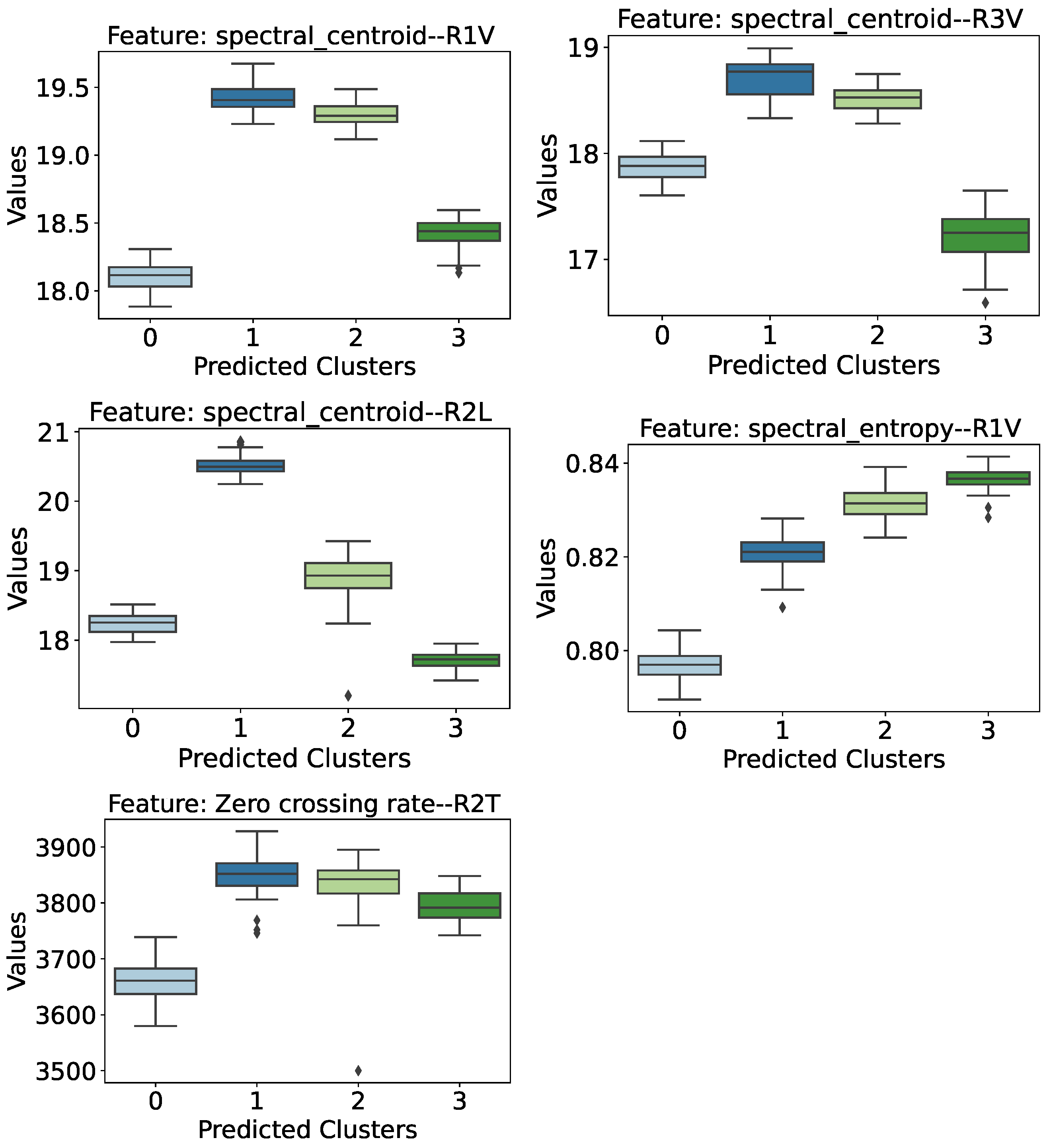
• Spectral Centroid (R1 Sensor): This attribute also shows near-separability between the cases of intact and damaged structures, except for a small overlap of intervals between the distribution of the intact structure (cluster 0) and the structure with the greatest severity of damage (cluster 3). However, if we analyze only the damaged cases, there is a certain tendency for the spectral centroid values to decrease as the severity of the damage increases.
• Spectral Centroid (R3 Sensor): The spectral centroid from the perspective of the R3 sensor shows almost total separability of the clusters, except for cluster 0 (healthy structure) having a small overlapping interval with the distribution of cluster 3 (lowering of 95 mm). Despite this, the behavior of the damaged structure cases is similar to that observed by the R1 sensor, i.e., the spectral centroid medians show a downward trend as the severity of the structure increases.
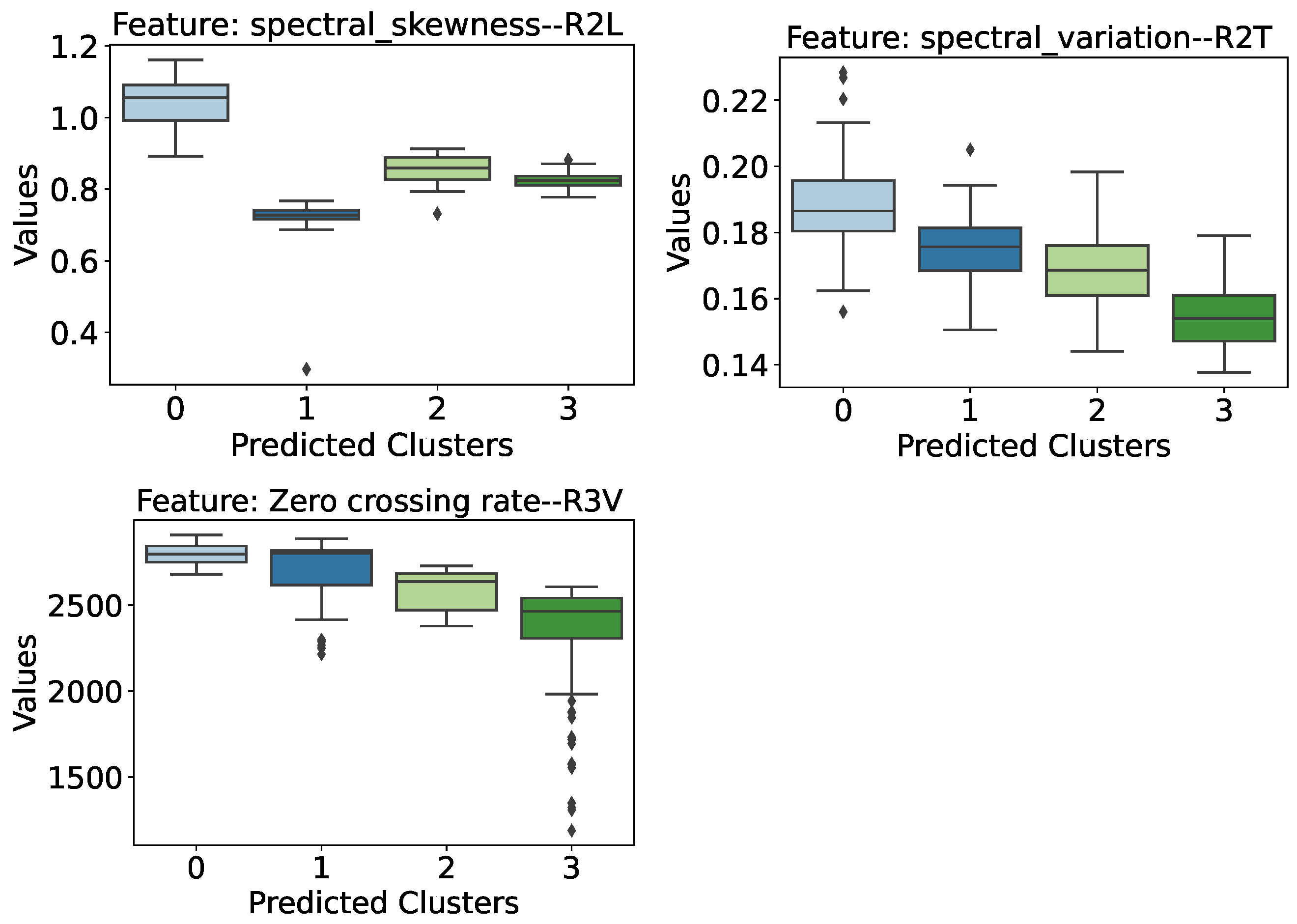
• Spectral Centroid (R2 Longitudinal Sensor): When analyzing the spectral centroids again, this time from the perspective of the R2 Longitudinal (R2L) Sensor, and discarding the distribution referring to the healthy structure, it is possible to see a clear trend and separability between the three levels of damage to the structure. Thus, when considering a damaged structure from the perspective of the R2L accelerometer, the greater the degree of severity of the damage, the lower its spectral centroid value tends to be.
• Spectral Entropy (R1 Sensor): This attribute deserves to be highlighted, because as well as being able to identify the presence of damage to the structure with a relatively safe margin, the behavior of the distributions also reveals a tendency for spectral entropy to increase as the degree of severity of the damage increases. Thus, the healthy structure of the Z24 bridge has low spectral entropy values, while the introduction of damage causes an increase in this value in proportion to its severity, i.e., the greater the severity of the damage, the higher the spectral entropy values.
• Zero Crossing Rate (R2 Transversal Sensor): This feature manages to separate cases of intact structure from cases of damaged structure, albeit with a narrower margin of difference. Thus, the bridge’s healthy structure is associated with lower Zero Crossing Rate values, while damaged structures have higher values. Furthermore, it is possible to see a certain trend in the damaged cases, so that the greater the severity of the damage, the lower the rate at which the vibration signal crosses the abscissa axis (coordinate axis equal to 0).

Finally, Figure 28 illustrates some less-prominent attributes, which can provide valuable insights. The spectral skewness observed from the perspective of the R2 Longitudinal Sensor shows an almost separability between the cases of the healthy and damaged structure, except for a small overlap of intervals between the healthy structure and the damaged one with 80 mm of lowering (cluster 2). The Spectral Variation and Zero Crossing Rate attributes, observed, respectively, from the perspective of the R2 Transversal and R3 sensors, reveal a very similar behavior. As the level of damage to the structure increases, the values of these attributes tend to decrease. Thus, a healthy structure would have the highest values, while a structure with a higher severity level would have the lowest values.

6.4. Performance Comparison

A comparison with the results of other papers in the literature could not be carried out, as, to the best of the authors’ knowledge, a clustering approach has not yet been evaluated in the case studies concerning the slender two-story aluminum structure (Section 5.1) and wall monitoring using the vibration response of a smartphone (Section 5.2. Regarding the Z24 benchmark dataset (Section 5.3), although it has been extensively evaluated in the literature from different perspectives of unsupervised learning, including clustering algorithms [62], the performance metrics generally adopted differ from those we used in this research (for example, [37,63]), as different evaluation approaches may require different performance measures.

In this sense, in order to compare our strategy with another unsupervised method commonly used in SHM problems, we chose to compare our results with those obtained by another clustering algorithm, known as Density-Based Spatial Clustering of Applications with Noise (DBSCAN) [64]. In this experiment, we configured the grid search to optimize the maximum distance between two samples ($eps$) and the metric to use when calculating distance between instances ($metric$), limiting the search conditions to the following values: $eps=[0.1,0.5,1,10]$ and $metric=[\mathit{Euclidean},L1,L2,\mathit{Manhattan},\mathit{Cosine}]$. No other adjustments were made to the parameters, with the exception of the selection threshold for the wall monitoring damage severity identification case (Section 5.2.2), which was changed from 0.90 to 0.87, and the wall monitoring anomaly detection for the Baker Hall material, which was changed from 0.8 to 0.73, as this adjustment was necessary. Finally, the results obtained in this experiment, before and after the selection of features, are shown in

Table 10. Averaged performance metrics compared across different scenarios achieved by the DBSCAN algorithm. The entries are labeled as a/b to distinguish the scenarios of the analysis. Specifically, “a” represents the results before feature selection, and “b” corresponds to the results after feature selection.

			Adjusted
Case Study	Homogeneity	Completeness	Rand Score	V-Measure
Aluminum Frame	1.0/1.0	1.0/1.0	1.0/1.0	1.0/1.0
Wall Monitoring (I)
Baker Bricks	0.9804/1.0	0.8974/1.0	0.9536/1.0	0.9337/1.0
Baker Hall	0.6541/1.0	0.5796/7107	0.6387/0.8450	0.6042/0.8308
Office Wall	0.9809/0.9798	0.8839/0.8801	0.9637/0.9531	0.9244/0.9255
Wall Monitoring (II)
Damage Severity	0.8783/0.9258	0.6784/0.7217	0.7189/0.7810	0.7651/0.8108
Z24 Bridge	0.8293/0.8196	0.9957/0.9880	0.8026/0.7959	0.9003/0.8884

.

By comparing the results obtained by DBSCAN—Table 10, it is possible to see that the agglomerative model used in this research tends to obtain higher clustering performances. Even though the performances were similar in some cases, such as in the aluminum frame case, these issues may be related to the data quality, because in this case study, the data were collected in a controlled environment. Therefore, when taking more complex cases, such as the Z24 bridge, the superiority of the agglomerative model can be seen more clearly when comparing the average clustering performances: Homogeneity = $0.9925/0.9987\times 0.8293/0.8196$; Completeness = $0.9926/0.9987\times 0.9957/0.9880$; Adjusted Rand score = $0.9944/0.9991\times 0.8026/0.7957$; V-measure = $0.9926/0.9987\times 0.9003/0.8884$.

Furthermore, in most cases, the feature selection process enhanced DBSCAN’s performance, similar to the results observed with the agglomerative model. In cases where performance improvement was not evident, the differences in the average metric values before and after feature selection were not statistically significant. The largest observed difference was 1.19% in the V-measure metric for the Z24 bridge case study.

6.5. Model Strengths and Limitations

The proposed model is based on assumptions about its ability to detect and analyze structural conditions. It assumes that vibration-based features provide a reliable way to monitor structural health by capturing important information about how a structure behaves under dynamic conditions. This aligns with common practices in SHM research, where features like time-based, statistical, and frequency-based data are used to identify damage. Despite its strengths, the model has some limitations, i.e., it depends on the quality and relevance of the features it selects, and external factors like temperature changes or varying loads, which can introduce noise into the data, making it harder to detect problems accurately.

Differences in performance between case studies highlight both physical and technical factors at play. For example, in a controlled laboratory setting, such as the two-story aluminum frame experiment, the clean and consistent data made it easier to accurately group structural conditions. However, in real-world cases, such as monitoring walls made from different materials, the model was affected by how changes in material stiffness due to damage could resemble natural differences between materials. This made it harder to separate damaged from undamaged states.

Although we did not face any major difficulties in running the agglomerative clustering on the databases used in this work, we realized that this model has a limitation in terms of computational cost, especially when applied to large datasets, once it has a time complexity of $O\left(N^3\right)$ and space complexity of $O\left(N^2\right)$. In this sense, determining a threshold for the extent to which this method is no longer viable and proposing alternatives for reducing the computational cost could be explored in future works.

Regarding the dimensionality reduction, we understand that for the adopted methodology and with the respective high performance achieved, the use of PCA was sufficient and it was not necessary to use more sophisticated techniques, such as the non-linear methods (e.g., t-SNE, Isomap, or UMAP). However, variants of the presented methodology can be developed in cases where the use of PCA does not lead to a reduced set of parameters that allow for good performance in classifications.

While the model successfully reduces data size and makes results easier to understand through feature selection, its ability to handle different structures and environments could be improved. Future works should focus on refining the model to better handle environmental variations and incorporate more physical insights into how structures behave. These improvements could make the model even more reliable and applicable across a wider range of SHM scenarios.

Finally, despite the positive findings of this study, the authors emphasize the need for further evaluations of case studies in other contexts, such as the detection of anomalies in machinery or rotating components, and also health data such as vital signs, electrocardiograms (ECGs), or even voice/cough recordings. The authors also encourage future works to evaluate state-of-the-art clustering methods and unsupervised feature selection approaches. Furthermore, as the proposed model is limited regarding the manual choice of threshold for selecting features, we suggest that future research further investigates this boundary condition, aiming to automate this identification.

7. Concluding Remarks and Future Works

This paper presented an unsupervised learning approach based on agglomerative clustering for vibration-based structural health monitoring. Data from dynamic tests from different civil structures were used for anomaly and damage severity detections. Also, an unsupervised feature selection approach based on box-plot statistics was proposed and evaluated in those SHM contexts. Four extrinsic metrics were used to assess the proposed approach.

The high clustering performances obtained in the four case studies allow us to draw the following conclusions:

• The agglomerative clustering combined with the unsupervised feature selection approach proved to be an effective unsupervised model for SHM tasks;
• The introduced unsupervised feature selection approach proved to be an efficient process for reducing data dimensionality and improving both clustering performance and interpretation.

Thus, the main contribution of this paper consists of the proposed approach finding a reduced set of dynamic signal characteristics capable of improving clustering performance and increasing the explainability of the machine learning model. This aspect is relevant because it minimizes user intervention and requires less specialist knowledge, as it provides an estimate of the most relevant features and their differences in visual plots.

Finally, despite the method showing promising results, further theoretical investigation is needed to establish a more robust foundation, particularly regarding the sensitivity of the clustering process to varying conditions. The automation of feature selection thresholds remains an open challenge. Although the current approach reduces dimensionality effectively, it requires user-defined thresholds, which may limit scalability in large-scale applications. Addressing this issue would enhance the method’s usability and adaptability. Therefore, the following points are suggested for future works:

• Theoretical improvements: Develop a more robust theoretical framework to enhance the stability and reliability of the clustering algorithm under diverse conditions.
• Adaptive automation: Investigate adaptive thresholding techniques for feature selection, enabling a fully automated process that minimizes user intervention and enhances scalability.
• Real-world validation: Conduct extensive evaluations of the method in specific application scenarios, such as bridge monitoring and industrial machinery health tracking, to validate its applicability and performance in practical settings.
• Integration with other techniques: Explore the integration of the proposed method with other machine learning techniques, such as semi-supervised and reinforcement learning, to address a wider range of SHM problems.
• Scalability studies: Examine the performance of the method on large and complex datasets to ensure its suitability for real-time SHM systems.

References

1. Farrar, C.R.; Worden, K. An introduction to structural health monitoring. Philos. Trans. R. Soc. Math. Phys. Eng. Sci. 2007, 365, 303–315. [Google Scholar] [CrossRef]
2. Rytter, A. Vibrational Based Inspection of Civil Engineering Structures. Ph.D. Thesis, Aalborg University, Aalborg, Denmark, 1993; 206p. [Google Scholar]
3. Sarmadi, H.; Entezami, A.; Ghalehnovi, M. On model-based damage detection by an enhanced sensitivity function of modal flexibility and LSMR-Tikhonov method under incomplete noisy modal data. Eng. Comput. 2020, 38, 111–127. [Google Scholar] [CrossRef]
4. Chen, Z.; Wang, Y.; Wu, J.; Deng, C.; Hu, K. Sensor data-driven structural damage detection based on deep convolutional neural networks and continuous wavelet transform. Appl. Intell. 2021, 51, 5598–5609. [Google Scholar] [CrossRef]
5. Alves, V.; Cury, A. An automated vibration-based structural damage localization strategy using filter-type feature selection. Mech. Syst. Signal Process. 2023, 190, 110145. [Google Scholar] [CrossRef]
6. Yang, Y.; Zhang, Y.; Tan, X. Review on Vibration-Based Structural Health Monitoring Techniques and Technical Codes. Symmetry 2021, 13, 1998. [Google Scholar] [CrossRef]
7. Xu, N.; Zhang, Z.; Liu, Y. 14—Spatiotemporal fractal manifold learning for vibration-based structural health monitoring. In Structural Health Monitoring/Management (SHM) in Aerospace Structures; Yuan, F.G., Ed.; Woodhead Publishing Series in Composites Science and Engineering; Woodhead Publishing: Cambridge, UK, 2024; pp. 409–426. [Google Scholar] [CrossRef]
8. Kauss, K.; Alves, V.; Barbosa, F.; Cury, A. Semi-supervised structural damage assessment via autoregressive models and evolutionary optimization. Structures 2024, 59, 105762. [Google Scholar] [CrossRef]
9. Goodfellow, I.; Bengio, Y.; Courville, A. Deep Learning; MIT Press: Cambridge, MA, USA, 2016. [Google Scholar]
10. Hastie, T.; Tibshirani, R.; Friedman, J. The Elements of Statistical Learning: Data Mining, Inference, and Prediction; Springer series in statistics; Springer: Cham, Switzerland, 2009. [Google Scholar]
11. Omori Yano, M.; Figueiredo, E.; da Silva, S.; Cury, A. Foundations and applicability of transfer learning for structural health monitoring of bridges. Mech. Syst. Signal Process. 2023, 204, 110766. [Google Scholar] [CrossRef]
12. Bodini, M. A Review of Facial Landmark Extraction in 2D Images and Videos Using Deep Learning. Big Data Cogn. Comput. 2019, 3, 14. [Google Scholar] [CrossRef]
13. Krishnanunni, C.G.; Raj, R.S.; Nandan, D.; Midhun, C.K.; Sajith, A.S.; Ameen, M. Sensitivity-based damage detection algorithm for structures using vibration data. J. Civ. Struct. Health Monit. 2018, 9, 137–151. [Google Scholar] [CrossRef]
14. Mekjavić, I.; Damjanović, D. Damage Assessment in Bridges Based on Measured Natural Frequencies. Int. J. Struct. Stab. Dyn. 2017, 17, 1750022. [Google Scholar] [CrossRef]
15. Ciambella, J.; Pau, A.; Vestroni, F. Modal curvature-based damage localization in weakly damaged continuous beams. Mech. Syst. Signal Process. 2019, 121, 171–182. [Google Scholar] [CrossRef]
16. Finotti, R.P.; Souza Barbosa, F.; Cury, A.A.; Gentile, C. A novel natural frequency-based technique to detect structural changes using computational intelligence. Procedia Eng. 2017, 199, 3314–3319. [Google Scholar] [CrossRef]
17. Salawu, O. Detection of structural damage through changes in frequency: A review. Eng. Struct. 1997, 19, 718–723. [Google Scholar] [CrossRef]
18. Resende, L.; Finotti, R.; Barbosa, F.; Garrido, H.; Cury, A.; Domizio, M. Damage identification using convolutional neural networks from instantaneous displacement measurements via image processing. Struct. Health Monit. 2023, 23, 1627–1640. [Google Scholar] [CrossRef]
19. Abdeljaber, O.; Avci, O.; Kiranyaz, S.; Gabbouj, M.; Inman, D.J. Real-time vibration-based structural damage detection using one-dimensional convolutional neural networks. J. Sound Vib. 2017, 388, 154–170. [Google Scholar] [CrossRef]
20. Sony, S.; Gamage, S.; Sadhu, A.; Samarabandu, J. Vibration-based multiclass damage detection and localization using long short-term memory networks. Structures 2022, 35, 436–451. [Google Scholar] [CrossRef]
21. Finotti, R.P.; Barbosa, F.S.; Cury, A.A.; Pimentel, R.L. Numerical and Experimental Evaluation of Structural Changes Using Sparse Auto-Encoders and SVM Applied to Dynamic Responses. Appl. Sci. 2021, 11, 11965. [Google Scholar] [CrossRef]
22. Finotti, R.P.; Gentile, C.; Barbosa, F.; Cury, A. Structural novelty detection based on sparse autoencoders and control charts. Struct. Eng. Mech. 2022, 81, 647–664. [Google Scholar] [CrossRef]
23. Finotti, R.P.; Barbosa, F.S.; Cury, A.A.; Pimentel, R.L. Novelty Detection Using Sparse Auto-Encoders to Characterize Structural Vibration Responses. Arab. J. Sci. Eng. 2022, 47, 13049–13062. [Google Scholar] [CrossRef]
24. Spínola Neto, M.; Finotti, R.; Barbosa, F.; Cury, A. Structural Damage Identification Using Autoencoders: A Comparative Study. Buildings 2024, 14, 2014. [Google Scholar] [CrossRef]
25. Finotti, R.P.; Cury, A.A.; Barbosa, F.S. An SHM approach using machine learning and statistical indicators extracted from raw dynamic measurements. Lat. Am. J. Solids Struct. 2019, 16, e165. [Google Scholar] [CrossRef]
26. Pan, H.; Azimi, M.; Yan, F.; Lin, Z. Time-Frequency-Based Data-Driven Structural Diagnosis and Damage Detection for Cable-Stayed Bridges. J. Bridge Eng. 2018, 23, 04018033. [Google Scholar] [CrossRef]
27. Yang, Y.; Nagarajaiah, S. Blind identification of damage in time-varying systems using independent component analysis with wavelet transform. Mech. Syst. Signal Process. 2014, 47, 3–20. [Google Scholar] [CrossRef]
28. Kankanamge, Y.; Hu, Y.; Shao, X. Application of wavelet transform in structural health monitoring. Earthq. Eng. Eng. Vib. 2020, 19, 515–532. [Google Scholar] [CrossRef]
29. Avci, O.; Abdeljaber, O.; Kiranyaz, S.; Hussein, M.; Gabbouj, M.; Inman, D.J. A review of vibration-based damage detection in civil structures: From traditional methods to Machine Learning and Deep Learning applications. Mech. Syst. Signal Process. 2021, 147, 107077. [Google Scholar] [CrossRef]
30. Abu-Mahfouz, I.; Banerjee, A. Crack Detection and Identification Using Vibration Signals and Fuzzy Clustering. Procedia Comput. Sci. 2017, 114, 266–274. [Google Scholar] [CrossRef]
31. Lucà, F.; Manzoni, S.; Cerutti, F.; Cigada, A. A Damage Detection Approach for Axially Loaded Beam-like Structures Based on Gaussian Mixture Model. Sensors 2022, 22, 8336. [Google Scholar] [CrossRef]
32. Entezami, A.; Shariatmadar, H.; Karamodin, A. Improving feature extraction via time series modeling for structural health monitoring based on unsupervised learning methods. Sci. Iran. 2020, 27, 1001–1018. [Google Scholar] [CrossRef]
33. Alves, V.; Cury, A.; Roitman, N.; Magluta, C.; Cremona, C. Novelty detection for SHM using raw acceleration measurements. Struct. Control. Health Monit. 2015, 22, 1193–1207. [Google Scholar] [CrossRef]
34. Khoa, N.L.; Zhang, B.; Wang, Y.; Chen, F.; Mustapha, S. Robust dimensionality reduction and damage detection approaches in structural health monitoring. Struct. Health Monit. 2014, 13, 406–417. [Google Scholar] [CrossRef]
35. Entezami, A.; Sarmadi, H.; Behkamal, B. Long-term health monitoring of concrete and steel bridges under large and missing data by unsupervised meta learning. Eng. Struct. 2023, 279, 115616. [Google Scholar] [CrossRef]
36. Delgadillo, R.M.; Casas, J.R. SHM of Bridges by Improved Complete Ensemble Empirical Mode Decomposition with Adaptive Noise (ICEEMDAN) and Clustering. Struct. Health-Monit.-Int. J. 2019. [Google Scholar] [CrossRef]
37. Civera, M.; Sibille, L.; Zanotti Fragonara, L.; Ceravolo, R. A DBSCAN-based automated operational modal analysis algorithm for bridge monitoring. Measurement 2023, 208, 112451. [Google Scholar] [CrossRef]
38. Roveri, N.; Milana, S.; Culla, A.; Conte, P.; Pepe, G.; Mezzani, F.; Carcaterra, A. Machine learning and sensor swarm for structural health monitoring of a bridge. In Proceedings of the ISMA 2020—International Conference on Noise and Vibration Engineering and USD 2020—International Conference on Uncertainty in Structural Dynamics, Virtual, 7–9 September 2020; pp. 2817–2824. [Google Scholar]
39. Diez, A.; Khoa, N.L.D.; Makki Alamdari, M.; Wang, Y.; Chen, F.; Runcie, P. A clustering approach for structural health monitoring on bridges. J. Civ. Struct. Health Monit. 2016, 6, 429–445. [Google Scholar] [CrossRef]
40. Chen, S.; Ong, Z.C.; Lam, W.H.; Lim, K.S.; Lai, K.W. Unsupervised Damage Identification Scheme Using PCA-Reduced Frequency Response Function and Waveform Chain Code Analysis. Int. J. Struct. Stab. Dyn. 2020, 20, 2050091. [Google Scholar] [CrossRef]
41. Siow, P.Y.; Ong, Z.C.; Khoo, S.Y.; Lim, K.S. Damage Sensitive PCA-FRF Feature in Unsupervised Machine Learning for Damage Detection of Plate-Like Structures. Int. J. Struct. Stab. Dyn. 2021, 21, 2150028. [Google Scholar] [CrossRef]
42. Diday, E.; Noirhomme-Fraiture, M. Symbolic Data Analysis and the SODAS Software; Wiley-Interscience: Hoboken, NJ, USA, 2008. [Google Scholar]
43. Hassan Daneshvar, M.; Sarmadi, H. Unsupervised learning-based damage assessment of full-scale civil structures under long-term and short-term monitoring. Eng. Struct. 2022, 256, 114059. [Google Scholar] [CrossRef]
44. Ackermann, M.R.; Blömer, J.; Kuntze, D.; Sohler, C. Analysis of Agglomerative Clustering. Algorithmica 2012, 69, 184–215. [Google Scholar] [CrossRef]
45. Tokuda, E.K.; Comin, C.H.; Costa, L.d.F. Revisiting agglomerative clustering. Phys. A Stat. Mech. Its Appl. 2022, 585, 126433. [Google Scholar] [CrossRef]
46. Jolliffe, I. Principal Component Analysis; Springer Verlag: New York, NY, USA, 2002. [Google Scholar]
47. Vyas, S.; Kumaranayake, L. Constructing socio-economic status indices: How to use principal components analysis. Health Policy Plan. 2006, 21, 459–468. [Google Scholar] [CrossRef]
48. Rosenberg, A.; Hirschberg, J. V-Measure: A Conditional Entropy-Based External Cluster Evaluation Measure. In Proceedings of the 2007 Joint Conference on Empirical Methods in Natural Language Processing and Computational Natural Language Learning (EMNLP-CoNLL), Prague, Czech Republic, 28–30 June 2007; pp. 410–420. [Google Scholar]
49. Barandas, M.; Folgado, D.; Fernandes, L.; Santos, S.; Abreu, M.; Bota, P.; Liu, H.; Schultz, T.; Gamboa, H. TSFEL: Time Series Feature Extraction Library. SoftwareX 2020, 11, 100456. [Google Scholar] [CrossRef]
50. Virtanen, P.; Gommers, R.; Oliphant, T.E.; Haberland, M.; Reddy, T.; Cournapeau, D.; Burovski, E.; Peterson, P.; Weckesser, W.; Bright, J.; et al. SciPy 1.0: Fundamental Algorithms for Scientific Computing in Python. Nat. Methods 2020, 17, 261–272. [Google Scholar] [CrossRef]
51. Crutchfield, J.P.; Feldman, D.P. Regularities unseen, randomness observed: Levels of entropy convergence. Chaos Interdiscip. J. Nonlinear Sci. 2003, 13, 25–54. [Google Scholar] [CrossRef]
52. McKinney, W. Data Structures for Statistical Computing in Python. In Proceedings of the 9th Python in Science Conference, Austin, TX, USA, 28 June–3 July 2010; pp. 56–61. [Google Scholar] [CrossRef]
53. Harris, C.R.; Millman, K.J.; van der Walt, S.J.; Gommers, R.; Virtanen, P.; Cournapeau, D.; Wieser, E.; Taylor, J.; Berg, S.; Smith, N.J.; et al. Array programming with NumPy. Nature 2020, 585, 357–362. [Google Scholar] [CrossRef]
54. Hunter, J.D. Matplotlib: A 2D graphics environment. Comput. Sci. Eng. 2007, 9, 90–95. [Google Scholar] [CrossRef]
55. Waskom, M.L. seaborn: Statistical data visualization. J. Open Source Softw. 2021, 6, 3021. [Google Scholar] [CrossRef]
56. Pedregosa, F.; Varoquaux, G.; Gramfort, A.; Michel, V.; Thirion, B.; Grisel, O.; Blondel, M.; Prettenhofer, P.; Weiss, R.; Dubourg, V.; et al. Scikit-learn: Machine Learning in Python. J. Mach. Learn. Res. 2011, 12, 2825–2830. [Google Scholar]
57. Finotti, R.P.; Silva, C.F.; Oliveira, P.H.E.; Barbosa, F.S.; Cury, A.A.; Silva, R.C. Novelty detection on a laboratory benchmark slender structure using an unsupervised deep learning algorithm. Lat. Am. J. Solids Struct. 2023, 20, e512. [Google Scholar] [CrossRef]
58. Sun, W. VibWall: Smartphone’s Vibration Challenge-response for Wall Crack Detection. ACM J. Comput. Sustain. Soc. 2023, 1, 1–24. [Google Scholar] [CrossRef]
59. Maeck, J.; De Roeck, G. Description of Z24 benchmark. Mech. Syst. Signal Process. 2003, 17, 127–131. [Google Scholar] [CrossRef]
60. Roeck, G.D.; Peeters, B.; Maeck, J. Dynamic monitoring of civil engineering structures. In Proceedings of the Computational Methods for Shell and Spatial Structures IASS-IACM 2000, Chania, Greece, 4–7 June 2000. [Google Scholar]
61. Sinou, J.J. A Review of Damage Detection and Health Monitoring of Mechanical Systems from Changes in the Measurement of Linear and Non-linear Vibrations. In Mechanical Vibrations: Measurement, Effects and Control; Nova Science: Hauppauge, NY, USA, 2009; pp. 643–702. [Google Scholar]
62. Eltouny, K.; Gomaa, M.; Liang, X. Unsupervised Learning Methods for Data-Driven Vibration-Based Structural Health Monitoring: A Review. Sensors 2023, 23, 3290. [Google Scholar] [CrossRef]
63. Silva, M.; Santos, A.; Figueiredo, E.; Santos, R.; Sales, C.; Costa, J.C. A novel unsupervised approach based on a genetic algorithm for structural damage detection in bridges. Eng. Appl. Artif. Intell. 2016, 52, 168–180. [Google Scholar] [CrossRef]
64. Ester, M.; Kriegel, H.P.; Sander, J.; Xu, X. A density-based algorithm for discovering clusters in large spatial databases with noise. In Proceedings of the Second International Conference on Knowledge Discovery and Data Mining, KDD’96, Portland, OR, USA, 2–4 August 1996; AAAI Press: Washington, DC, USA, 1996; pp. 226–231. [Google Scholar]
Figure 5. Illustration of the process of assigning weight to the importance of attributes. Non-overlapping intervals result in a bonus of 2 points, while non-overlapping interquartiles only result in 1 point.
Infrastructures 10 00032 g005
Figure 6. Flowchart of the methodological process used. The purple squares represent processes that were executed 5 times independently. The red line indicates a new round of independent runs of the computer model, considering the dataset formed by the selected features.
Infrastructures 10 00032 g006
Figure 7. Detailed illustration of the slender two-story aluminum structure used to acquire the experimental data [57].
Infrastructures 10 00032 g007
Figure 8. The wall sample built to be used in the context of estimating the severity of damage (crack depth) in a wall [58].
Infrastructures 10 00032 g008
Figure 9. Front, top, and cross-section view of Z24 bridge [59].
Infrastructures 10 00032 g009
Figure 10. Monitoring grid installed on the bridge. Adapted from [60].
Infrastructures 10 00032 g010
Figure 11. Features selected considering a selection threshold defined as 75 % of the maximum score. The number at the end of the attribute name indicates the accelerometer on which the attribute was evaluated.
Infrastructures 10 00032 g011
Figure 12. Accumulated confusion matrix of the 25 iterations of the model before the voting-based process for the two-story slender aluminum frame. It should be noted that after the voting-based process, the matrix remained unchanged.
Infrastructures 10 00032 g012
Figure 13. Distribution of the most relevant attribute values for accelerometer 1.
Infrastructures 10 00032 g013
Figure 14. Distribution of the most relevant attribute values for accelerometer 2.
Infrastructures 10 00032 g014
Figure 15. Distribution of the most relevant attribute values for accelerometers 3 and 4, which are identified in the title of the graph by the suffix “–3” and “–4”, respectively.
Infrastructures 10 00032 g015
Figure 16. Confusion matrix regarding Baker Bricks scenario.
Infrastructures 10 00032 g016
Figure 17. Confusion matrix regarding Baker Hall scenario.
Infrastructures 10 00032 g017
Figure 18. Confusion matrix regarding Office Wall scenario.
Infrastructures 10 00032 g018
Figure 19. Most relevant attributes regarding the Baker Bricks scenario. The number at the end of the feature name corresponds to the excitation vibration frequency for which the feature was evaluated.
Infrastructures 10 00032 g019
Figure 20. Most relevant attributes regarding the Baker Hall scenario. The number at the end of the feature name corresponds to the excitation vibration frequency for which the feature was evaluated.
Infrastructures 10 00032 g020
Figure 21. Behavior of the selected normalized features. The number at the end of the feature name corresponds to the excitation vibration frequency for which the feature was evaluated.
Infrastructures 10 00032 g021
Figure 22. Confusion matrix for damage severity identification in wall monitoring.
Infrastructures 10 00032 g022
Figure 23. Distribution of the most relevant features considering the predicted clusters. The number at the end of the feature name corresponds to the excitation vibration frequency for which the feature was evaluated.
Infrastructures 10 00032 g023
Figure 24. Features selected considering a selection threshold as 16 % of the maximum score. Each feature indicates the sensor to which it refers at the end of its name.
Infrastructures 10 00032 g024
Figure 25. Confusion matrix from bridge Z24 study case.
Infrastructures 10 00032 g025
Figure 26. Distribution of the most relevant features in the anomaly detection task, considering the predicted clusters. The sensor associated with the information retrieved from the signals is indicated at the end of the attribute name.
Infrastructures 10 00032 g026
Figure 27. Distribution of the most relevant features in the severity damage estimation task, considering the predicted clusters. The sensor associated with the information retrieved from the signals is indicated at the end of the attribute name.
Infrastructures 10 00032 g027
Figure 28. Distribution of the other features highlighted in the preliminary analysis, considering the predicted clusters. The sensor associated with the information retrieved from the signals is indicated at the end of the attribute name.
Infrastructures 10 00032 g028