Evaluating Factors Influencing Dynamic Modulus Prediction: GRA-MLR Compared with Sigmoidal Modelling for Asphalt Mixtures with Reclaimed Asphalt

Abstract

The dynamic modulus of asphalt mixtures (|E*|) is a key mechanical parameter in the design of road pavements, yet direct laboratory testing is time- and resource-intensive. This study evaluates two predictive models for estimating |E*| using data from 62 asphalt mixtures containing reclaimed asphalt: a grey relational analysis–multiple linear regression (GRA-MLR) hybrid model and a mechanistic sigmoidal model. The results showed that the GRA-MLR model effectively identifies influential variables but achieved moderate predictive accuracy (R² values varying from 0.4743 to 0.6547). In contrast, the sigmoidal model outperformed across all temperature conditions (R² > 0.96) and produced predictions deviating by less than ±20% from measured values. Temperature-dependent shifts in factor influence were observed, with stiffness and gradation dominating at low temperatures and reclaimed asphalt (RA) content becoming more significant at higher temperatures. While the GRA-MLR model is advantageous, offering rapid assessments and early-stage evaluations, the sigmoidal model offers the precision suited for detailed design. Integrating both models can balance computational efficiency and provide a balanced strategy, with strong predictive reliability to advance mechanistic–empirical pavement design.

1. Introduction

The dynamic modulus of asphalt mixtures (|E*|) is a key mechanical parameter in the design of road pavements, as it directly influences the long-term performance of pavements under traffic loads and varying environmental conditions. Recognizing its importance, many national guidelines—including the Mechanistic–Empirical Pavement Design Guide—have emphasized the need to accurately determine |E*| values in recent years [1]. Typically, the dynamic modulus can be obtained either through direct laboratory testing of asphalt mixtures or by prediction using empirical equations and models [2,3]. While direct laboratory testing is generally regarded as more accurate and precise, it is also resource-intensive, requiring specific sampling and testing at multiple temperatures and loading frequencies. As a result, this method can be both time- and material-intensive.

The availability of |E*| values is often limited, particularly for lower functional class pavement projects. Despite the existence of well-established laboratory-based testing procedures, these methods present several challenges, including lengthy test durations, high costs, and substantial labour requirements [4]. Such constraints often obstruct practitioners from acquiring reliable |E*| measurements during the preliminary design stages—especially when materials are not readily accessible or for lower-class pavement projects [5,6]. To address these limitations and support the needs of practitioners, researchers have developed alternative approaches for estimating |E*|, leading to the rise of various empirical and statistical models that offer simpler and more practical prediction methods.

Empirical equations primarily rely on observed data and correlations derived from laboratory or field test results rather than fundamental mechanistic principles. They are established from historical performance and test results to predict future pavement behaviour. These approaches frequently utilize both linear and non-linear regression techniques. When a single explanatory variable is used, the method is referred to as univariable regression; in contrast, the inclusion of multiple predictors constitutes multivariable regression. Given that pavement degradation is typically influenced by a combination of factors, univariable regression models often lack the complexity needed to yield accurate predictions [7].

Through the years, many studies have been conducted and significant efforts have been made to establish empirical models for forecasting different pavement conditions [8,9,10]. Among these, the dynamic modulus has been a key focus, with widely used models including those developed by Witczak, Hirsch, and Al-Khateeb [5,11,12,13]. Although they are simple and accessible, their reliance on the volumetric characteristics of compacted mixtures, aggregate gradation, binder properties, and test temperature can significantly vary their accuracy from one country to another [4,5,14]. Moreover, there is a lack of models accounting for reclaimed asphalt variability, which restricts their applicability in modern pavement design scenarios [1]. Because of these alterations and limitations, the application of predictive models should be adapted.

In addition, the investigation of factors impacting dynamic modulus has earned increased attention within the research community [2,14,15]. Furthermore, given its analytical strengths, grey relational theory has shown strong potential for screening the factors influencing dynamic modulus prediction models. Zhang et al. [14] developed a dynamic modulus prediction model for asphalt mixtures by combining grey relational analysis to identify key easily obtainable material factors and using multiple linear regression for model construction. The results showed that the model provided accurate predictions, demonstrating that the complex modulus and viscosity of the binder, as well as void characteristics, are the most influential parameters controlling the dynamic modulus of asphalt mixtures. Zheng et al. [16] used grey relational analysis to evaluate the relationship between the ultimate bending failure strength/strain and low-temperature crack resistance across different asphalt compositions under low-temperature conditions. Chen et al. [17] applied the grey target decision method to establish a comprehensive performance evaluation for tourmaline-modified asphalt mixtures. The results confirm the method’s reliability and suitability for practical applications. While previous studies mainly focus on the investigation of material characteristic factors in developing prediction models, few studies focus on the interaction between material properties and mechanical behaviour in the development of dynamic modulus prediction models using grey relational analysis.

This study aims to analyse and compare two predictive models—grey relational analysis–multiple linear regression hybrid model and a sigmoidal model—in a dataset of 62 asphalt mixtures with varying contents of reclaimed asphalt. The main objective of this comparison is to assess the mechanistic sigmoid model and the modern statistical GRA-MLR approaches in predicting dynamic modulus, with the goal of revealing their strengths and weaknesses. This is carried out by constructing the best model that meets the real-world needs of accuracy, adaptability to various asphalt mixtures, and ease of application.

2. Materials and Methods

2.1. Materials

2.1.1. Bituminous Binder

Two types of bituminous binders were used for this study. The first type includes neat binders (paving grades) with penetration of 50–70 and 70–100 0.1 mm at 25 °C. The second type is commercial polymer-modified bitumen (PMB), with a penetration of 25–55 0.1 mm at 25 °C and a softening point higher than 65 °C, as is used regularly in Czechia. For this latter requirement, two bituminous binders were used: a standard PMB as regulated by EN 14023 [18] and a PMB RC, which was specifically formulated for use with reclaimed asphalt materials, allowing for elevated RA content mixtures while maintaining road performance, sustainability, and long service life. This modified bituminous binder has a higher content of polymers, which will balance the polymers that are not contained by the binder in RA in mixtures with elevated reclaimed asphalt content. The physical properties of the utilized binders were verified and guaranteed to fulfil the requirements set by EN 12591 for net binders and by EN 14023 or CSN 657222-1 for PMBs [19,20].

2.1.2. Additives

In this study, a diverse range of additives was incorporated into asphalt mixtures to evaluate their effects on performance characteristics. These additives can be classified into four groups based on their chemical nature and functional role:

• Rejuvenating agents are generally composed of bio-based oils (like vegetable oils, fatty acids, triglycerides, and tall oils), petroleum-based oils (such as paraffinic, naphthenic, and aromatic oils), or engineered products, which are designed to restore the viscoelastic properties of aged binders [21,22] 1. In the present paper, a selection of bio-based, experimental, and commercial rejuvenating agents was evaluated.
• Low-density polyethylene (LDPE) is a thermoplastic polymer formed via the high-pressure polymerization of ethylene, and it is recognized as part of the solid waste stream associated with domestic goods [23,24]. It is used to enhance elasticity and resistance to deformation.
• Crumb rubber is derived from recycled tires that have been processed into particles < 0.8 mm after reaching the end of their life cycle. It is known for improving flexibility and fatigue resistance [25,26].
• Fibres are employed to improve tensile strength and resistance to cracking. The used fibres in asphalt mixtures are generally either organic (such as cellulose, polyester, aramid, and polypropylene fibres) or inorganic (such as glass and basalt fibres) [27]. Cellulose fibres from jute will be used in this research.

2.2. Specimen Preparation

A total of 62 asphalt concrete (AC) mixtures were investigated. They involved three kinds of grading, four types of bitumen, and four reclaimed asphalt contents. All asphalt mixtures included are representative of those commonly used in Czech pavement structures. This dataset was compiled from samples sourced either from laboratory-based research/mix design or commercial project collaborations produced by mixing plants. A summary of these mixtures is indicated in

Table 1. Samples of asphalt mixtures.

Mixture Type	Pavement Layer [28]	NMAS * (mm)	Reclaimed Asphalt Content (%)	Total Number
AC	Surface layer (“O”)	11	30%	6
	Binder layer (“L”)	16	40%	8
		16+	30%	8
			50%	38
		22	30%	2

* Nominal maximum aggregate size.

.

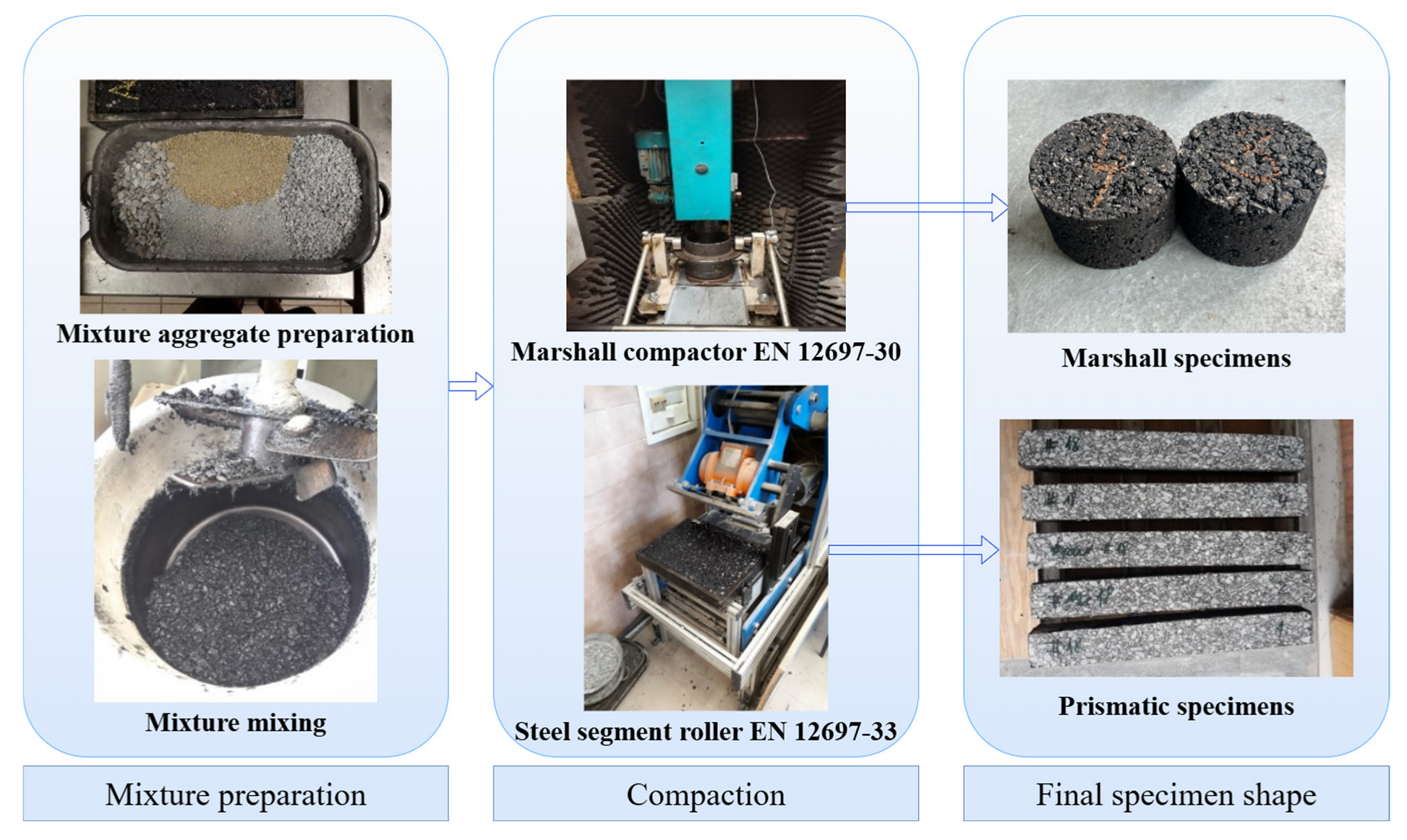
Two distinct specimen shapes were employed: Marshall (also commonly known as cylindrical) and prismatic specimens. Each sample geometry serves specific testing requirements and is manufactured using standardized compactions and cutting procedures. They were prepared according to the procedure shown in Figure 1. Marshall specimens are typically produced with a diameter of 100 mm and a height between 50 and 70 mm using a Marshall compactor. The procedure involves compacting hot asphalt mixtures in a mold with a mechanical Marshal hammer in accordance with the European standard EN 12697-30 [29]. Six replicas from the same batch of asphalt mixture were prepared. Prismatic specimens, on the other hand, are typically cut from compacted slabs using an asphalt saw to obtain samples with the following dimensions: 50 mm in height x 50 mm in width x 405 mm in length. Five testing samples were obtained from each asphalt slab. The slabs are produced using a steel segment roller in accordance with the European standard EN 12697-33 [30].

2.3. Study Methodology

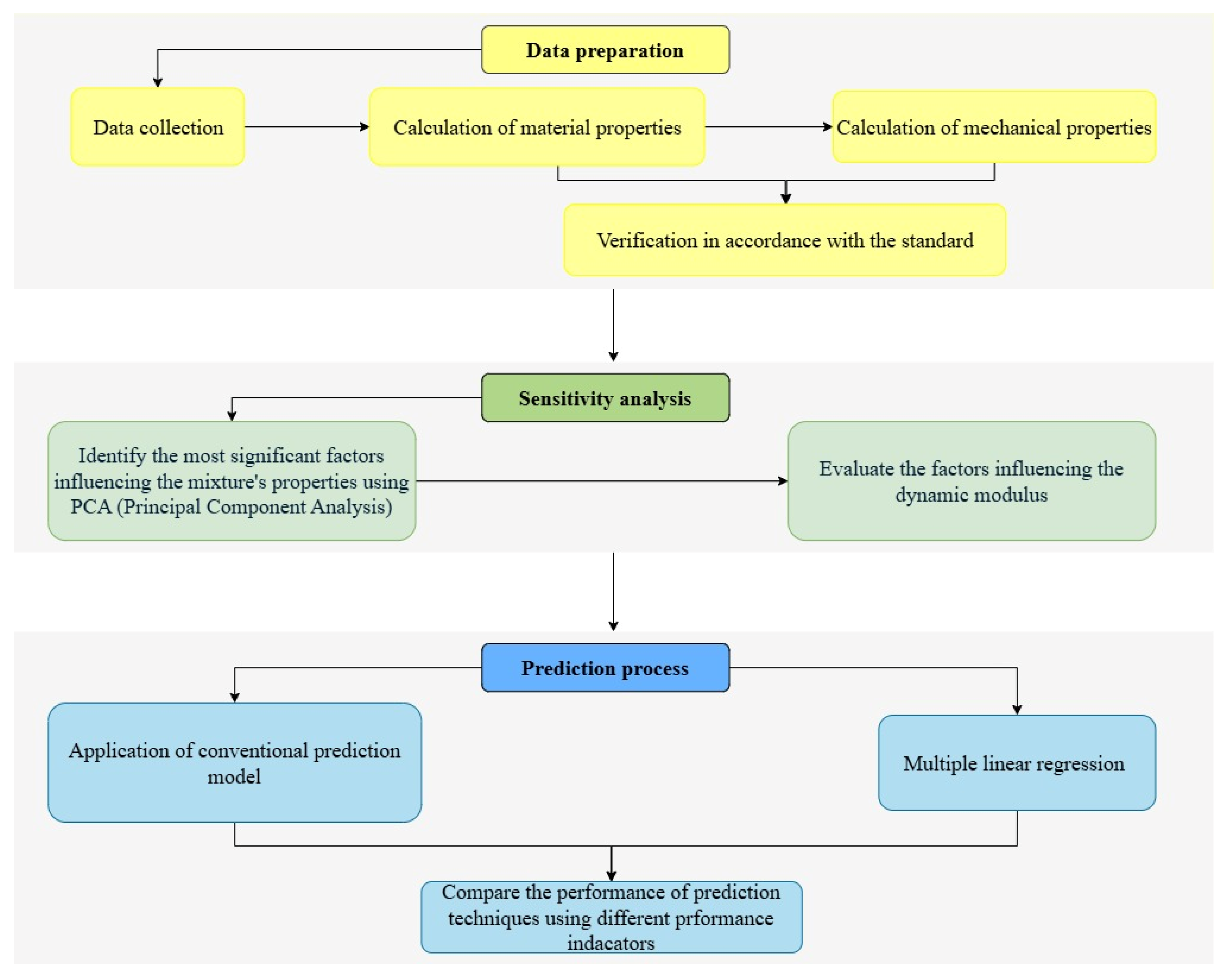
This study proposes a predictive approach for estimating the dynamic modulus of asphalt mixtures incorporating reclaimed asphalt. While the compressive rebound modulus is determined under static loading conditions, the dynamic modulus characterizes material behaviour under repeated cyclic loading and requires more advanced and precise testing instrumentation. In this research, a dataset of dynamic modulus values for selected mixtures was compiled and analysed using grey relational analysis (GRA) to identify the most influential material factors. Based on this analysis, a prediction model was developed through regression fitting and compared to a conventional prediction model. In the case of this study, the sigmoidal model for dynamic modulus prediction is calculated. The methodology flowchart is presented in Figure 2.

Based on the flowchart of this study, the primary density-related characteristics of the selected asphalt mixtures were investigated. These parameters are basic for evaluating the compaction quality of the mixtures and their internal structures. The maximum density, bulk density, and air void content (Va) were determined for all test specimens, as they serve as preliminary inputs for performance analysis and predictive modelling.

These parameters are interrelated parameters in asphalt mixture designs. Due to their mathematical interdependence, including all of them in the predictive model and in grey relational analysis may introduce redundancy, potentially distorting the interpretability of the statistical analysis. To address this, a principal component analysis (PCA) model was applied in this study to evaluate the degree of correlation among these variables and to extract the principal components that capture the most relevant variance in the data.

In fact, PCA is a statistical tool used for dimensionality reduction, pattern recognition, and exploratory data analysis. Its principal purpose is to reduce and simplify multivariate datasets (many variables) into a set of “principal components” with most of the data’s information. This allows for retaining sets with the most significant information whilst reducing redundancy and noise. It involves a sequence of linear operations. The following steps outline the PCA computation process:

• Standardization of the dataset

$$Z={\displaystyle \frac{X-\mu }{\sigma }}$$

(1)

where X is the original data matrix $(X=[x1,x2,x3]$, where each column represents a variable (maximum density, bulk density, and air void content)), μ is the mean of each variable, σ is the standard deviation of each variable, and Z is the standardized data matrix.

• Covariance matrix calculation

$$C={\displaystyle \frac{1}{n-1}}{Z}^{T}Z$$

(2)

• The Eigenvalue and Eigenvector decomposition are found by solving

$$C{e}_i={\lambda }_i{e}_i$$

(3)

where each eigenvalue ${\lambda }_i$ represents the amount of variance explained by its corresponding principal component, and each eigenvector $e_i$ represents a principal component direction.

• Percentage of variance explained

$$Explained\mathrm{ }variance\mathrm{ }ratio={\displaystyle \frac{{\lambda }_i}{\sum \lambda }}$$

(4)

This ratio is employed to determine how much information each principal component retains from the original dataset.

• Principal component scores

$$PC=Z\mathrm{ }{E}_k$$

(5)

Here, $E_k$ is the matrix of the top k eigenvectors, and PC is the new metric with the principal components.

In addition, the mechanical performance of asphalt mixtures was evaluated via two stiffness testing methods: the 4-point bending test on prismatic specimens (4 PB-PR) and the indirect tensile test on cylindrical specimens (IT-CY). The first was employed to measure the dynamic modulus by applying cyclic loads at two loading (upper) points while the beam is supported at two ends (lower points), inducing bending stresses in the middle region of the beam. This test was conducted at four controlled temperatures (0 °C, 10 °C, 20 °C, and 30 °C) and 11 frequencies (50, 30, 20, 15, 10, 8, 5, 3, 2, 1, and 0.1 Hz) in accordance with EN 12697-26 (Annex B), allowing for accurate determination of the dynamic modulus (|E*|) [31]. In contrast, the second test was conducted to assess the stiffness modulus by applying a compressive load across the vertical diameter of the specimen, inducing a horizontal tensile strain perpendicular to the loading direction. This procedure was conducted under three temperatures (0 °C, 15 °C, and 27 °C) in accordance with EN 12697-26 (Annex C), providing better insight into the tensile performance of asphalt mixtures [31].

Moreover, the 4PB-PR test provides higher accuracy and a more detailed characterisation of the viscoelastic performance of asphalt mixtures by simulating realistic bending stresses and temperature conditions. However, it requires more resources, advanced equipment, and longer test durations. In contrast, the IT-CY test is relatively less resource-intensive, simpler, faster, and requires less advanced equipment. However, it may provide a less comprehensive assessment of the asphalt mixture since it is less sensitive to characterizing complex material behaviour.

Consequently, an understanding of the relationship between these two tests can enable the more efficient use of static testing for predictive modelling. Therefore, within this study, an analysis of the influencing factors, including the static stiffness modulus, of the dynamic modulus is developed.

In this perspective, GRA was employed to investigate the influence of material parameters, such as maximum aggregate size (NMAS), binder content, binder grade, bulk density, maximum density, air void content, reclaimed asphalt content, additives, and static stiffness modulus, on the dynamic modulus of asphalt mixtures. GRA is another statistical tool; however, its main purpose is to evaluate and quantify the influence of multiple factors (input variables) on a target property (generally the performance variable of interest) through a normalized similarity comparison. In the context of asphalt mixture engineering, GRA is increasingly applied to assess and rank the influence of mix design parameters on a performance indicator such as the dynamic modulus—a key indicator of the mixture’s performance under traffic loading. The GRA process involves the following steps:

• Data normalization

Data normalization helps eliminate dimensional differences among variables. Based on a min–max value method, the normalizations were performed, referring to one of the three scenarios depending on each influencing factor.

For “higher is better”,

$$X_{ij}={\displaystyle \frac{x_{ij}-\min x_{ij}}{\max x_{ij}-\min x_{ij}}}$$

(6)

For “lower is better”,

$$X_{ij}={\displaystyle \frac{\max x_{ij}-x_{ij}}{\max x_{ij}-\min x_{ij}}}$$

(7)

For “nominal is better”,

$$X_{ij}=1-{\displaystyle \frac{\left|x_{ij}-x_{target}\right|}{\max \left|x_{ij}-x_{target}\right|}}$$

(8)

where $x_{ij}$ is the original value of the $i^{th}$ material parameters and the $j^{th}$ set of data, $X_{ij}$ is the normalized value of the correspondent matrix (from 0 to 1), $\min x_{ij}$ is the minimum value of the $x_{ij}$ matrix, $\max x_{ij}$ is the maximum value of the $x_{ij}$ matrix, and $x_{target}$ is the target value.

In this study, all raw data were normalized in accordance with the “higher is better” criterion.

• Reference and comparative sequences

The dynamic modulus sequence was defined as the reference sequence $X_{0j}$ while the above designated material parameter sequences were defined as the comparative sequences $X_{ij}$.

• Grey Relational Coefficient (GRC)

The grey relational coefficient is applied to determine the absolute difference between the normalized value and the reference sequence. It is calculated as

$${\xi }_{ij}\left(X_{0j}-X_{ij}\right)={\displaystyle \frac{{∆}_{min}+\mathrm{Ϛ}{∆}_{max}}{{∆}_{ij}+\mathrm{Ϛ}{∆}_{max}}}$$

(9)

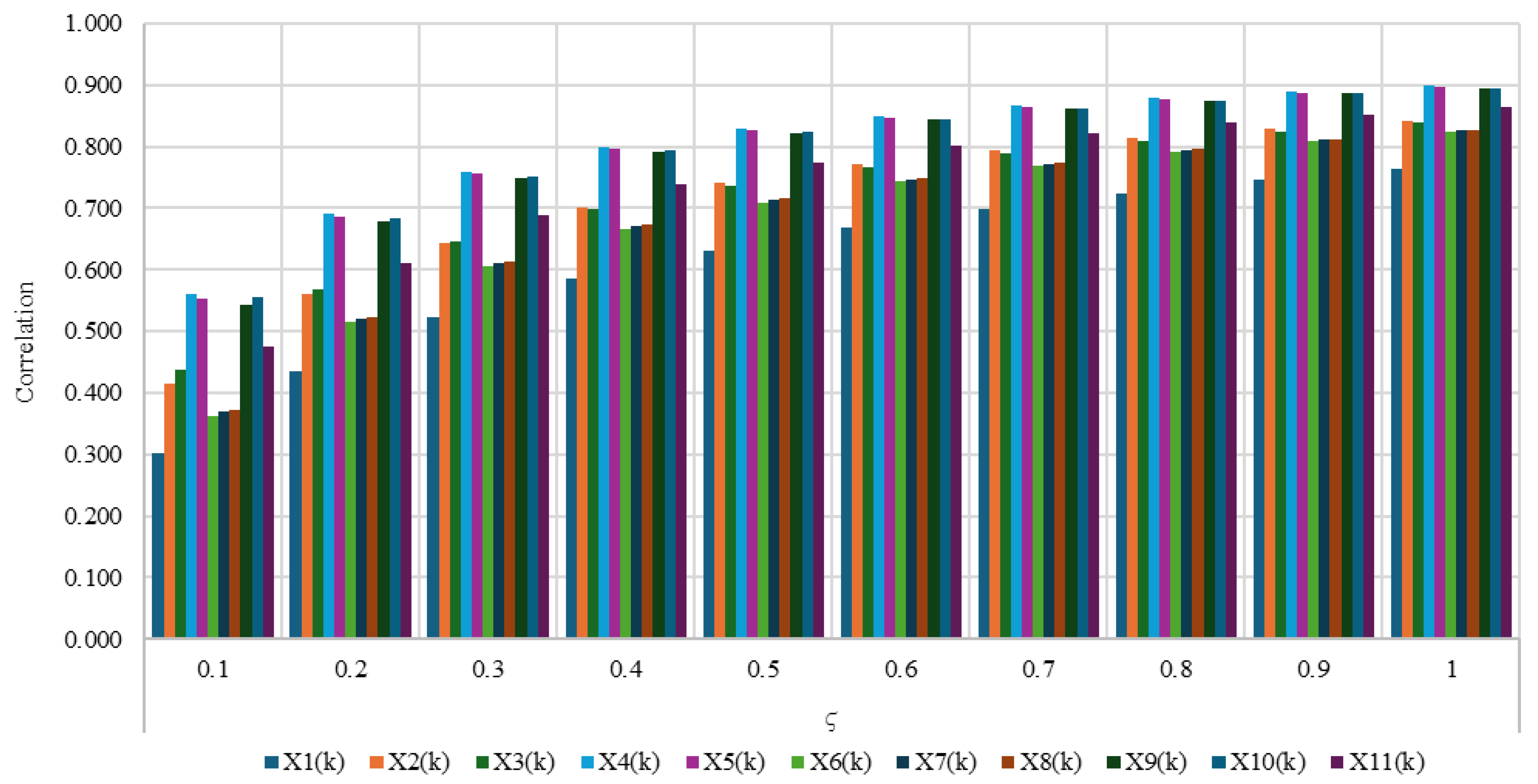
where ${∆}_{ij}$ is the absolute difference (${∆}_{ij}=|X_{0j}-X_{ij}|$), ${∆}_{min}$ is the minimum value of the ${∆}_{ij}$ matrix, ${∆}_{max}$ is the maximum value of the ${∆}_{ij}$ matrix, and $Ϛ$ is the resolution coefficient, which reflects the difference in the correlation ($0\le Ϛ\le 1$). In this research, through an analysis of all data, $Ϛ=0.4$ was considered. The results are summarized in Figure 3.

The sensitivity analysis across different ζ values (0.1–1.0) shows that the relative ranking of influential factors remains largely stable, indicating the robustness of the GRA results. However, at very low ζ values (e.g., 0.1–0.2), the differences between variables become exaggerated, whereas at high ζ values (e.g., >0.7), the distinctions among factors are compressed, reducing discriminatory power. A ζ value of 0.4 offers a balanced compromise, providing sufficient contrast between factors while maintaining stability across the dataset. Therefore, the choice of ζ = 0.4 can be justified as the most representative and reliable setting for capturing the relative influence of key mixture factors.

• Grey Relational Grade (GRG)

The grey relational grade represents the overall influence of the i^th factor on the performance matrix. A higher GRG indicates a stronger correlation between the input factor, i.e., the material parameter, and the output variable, i.e., the dynamic modulus. It is calculated as the average of the GRCs for each factor.

$${\gamma }_i={\displaystyle \frac{1}{n}}\sum _{k=1}^n{\mathrm{Ϛ}}_i\left(k\right)$$

(10)

3. Results and Discussion

3.1. Principal Component Analysis (PCA)

As described previously, the PCA model was employed to evaluate the degree of correlation among bulk density, maximum density, and air void content (analysed variables X₁, X₂, and X₃, respectively) and to extract the independent principal components. From

Table 2. Principal component analysis: eigenvalues and variance contribution.

Variable	Eigenvalue	Percentage Variance Explained (%)	Cumulative Percentage (%)
X1	0.003	0%	0%
X2	1.220	41%	41%
X3	1.777	59%	100%

, the explained variance rate of principal components 2 and 3 reached 41% and 59%, respectively, which indicated that these two principal components provide a comprehensive assessment of the material’s volumetric parameters. Consequently, within grey relational analysis, only the maximum density and air void content factors will be studied among the inputs.

3.2. Grey Relational Analysis Results

Table 3. Summary of the proportion of each factor at each temperature.

${\mathit{\gamma }}_{\mathit{i}}$	Influence Parameter	0 °C		10 °C		20 °C		30 °C
		GRG	Rank	GRG	Rank	GRG	Rank	GRG	Rank
${\mathit{\gamma }}_1$	RA content	0.764	11	0.595	11	0.651	5	0.609	6
${\mathit{\gamma }}_2$	Binder grade	0.843	6	0.674	6	0.623	6	0.549	8
${\mathit{\gamma }}_3$	Binder content	0.838	7	0.643	7	0.592	8	0.577	7
${\mathit{\gamma }}_4$	NMAS *	0.899	1	0.766	2	0.700	3	0.652	2
${\mathit{\gamma }}_5$	Additive content (rejuvenating agent)	0.897	2	0.781	1	0.727	1	0.780	1
${\mathit{\gamma }}_6$	Additive content (LDPE)	0.823	10	0.625	10	0.565	11	0.523	10
${\mathit{\gamma }}_7$	Additive content (crumb rubber)	0.826	9	0.628	9	0.567	10	0.520	11
${\mathit{\gamma }}_8$	Additive content (fibres)	0.827	8	0.633	8	0.577	9	0.534	9
${\mathit{\gamma }}_9$	Maximum density	0.895	4	0.765	3	0.722	2	0.652	3
${\mathit{\gamma }}_{10}$	Air void content	0.895	3	0.748	4	0.678	4	0.636	4
${\mathit{\gamma }}_{11}$	Static stiffness modulus	0.864	5	0.682	5	0.616	7	0.615	5

* Nominal maximum aggregate size.

presents the rankings of influencing factors based on their correlation coefficient with respect to the dynamic modulus at four temperatures. The results indicate that additive content, specifically rejuvenating agents, consistently exhibits the greatest influence on dynamic modulus at all temperatures, achieving the highest grey relational grade values and holding the top rank at each temperature. This is closely followed by NMAS and maximum density, both showing strong and stable correlations with respect to the dynamic modulus. On the other hand, factors such as RA content, LDPE, and crumb rubber additives show lower GRG values, suggesting a relatively weaker association with the modulus. The static stiffness modulus and air void content attain moderately high ranks, particularly at lower temperatures, showing their significance in stiffness behaviour. These results highlight the temperature-dependent influence of these parameters and underscore the predominant role of specific material characteristics, especially rejuvenating agents and aggregate gradation, in the mechanical performance of asphalt mixtures.

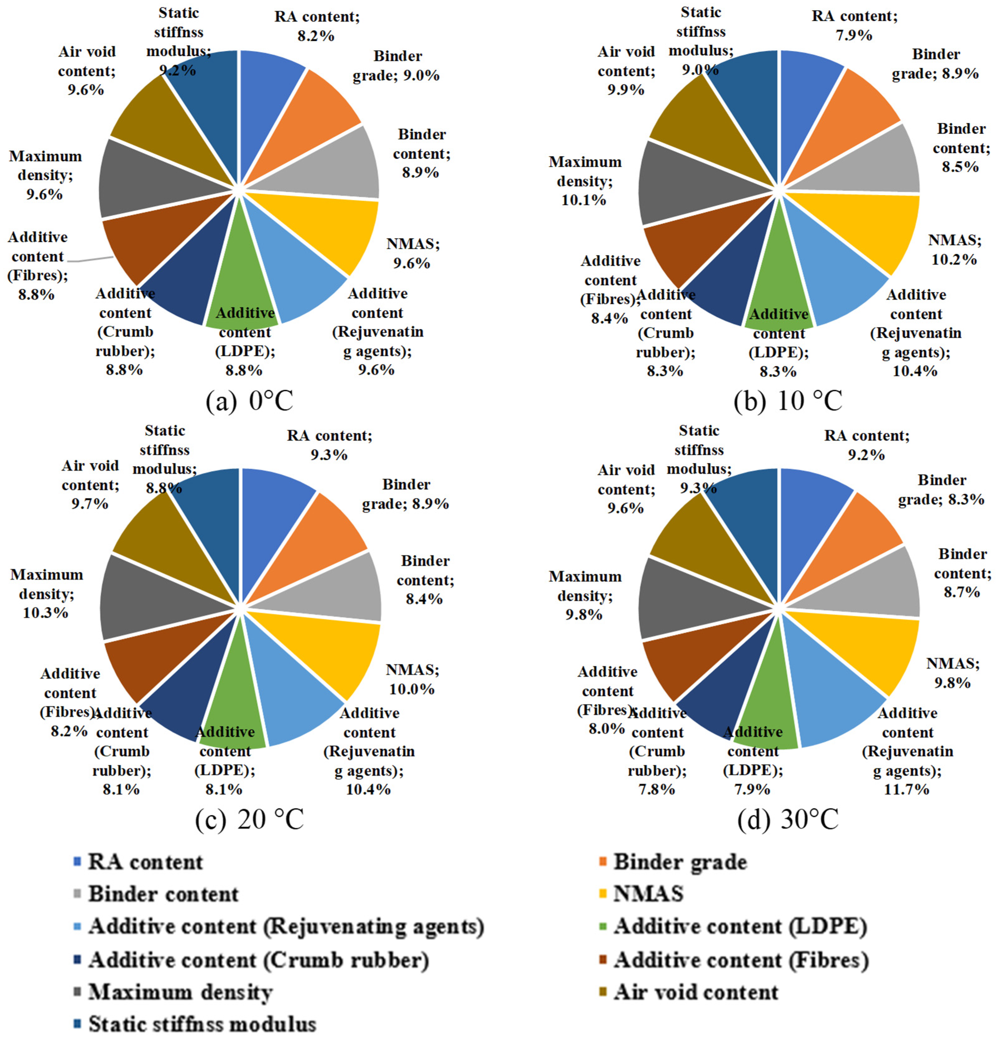
Figure 4 represents the proportional influence of eleven material parameters on the dynamic modulus at four temperatures using the GRA method. Similarly to the above results, rejuvenating agents were consistently the most influential factor across all temperatures. They reach a maximum share of 11.7% at 30 °C and maintain the highest or second-highest values at all temperatures. This indicates the significant role rejuvenating agents play in improving flexibility and restoring binder functionality, especially under high temperatures. However, additives such as LDPE, fibres, and crumb rubber show moderate-to-low contributions, suggesting a secondary but still significant influence on the dynamic modulus.

Parameters like NMAS, air void content, and maximum density show stable and relatively high distributions across the four temperatures, ranging between 9.6% and 10.3% and indicating their power in identifying the internal structure of asphalt mixtures.

The static stiffness modulus demonstrates moderate contributions across all temperatures, with influence rates between 8.8% at 20 °C and 9.3% at 30 °C.

Ultimately, the RA content shows the most variability among all the other parameters, showing a slightly higher effect at higher temperatures—9.3% and 9.2% at 20 °C and 30 °C, respectively, and 8.2% and 7.9% at 0 °C and 10 °C, respectively.

These findings emphasize the temperature-dependent nature shown previously and highlight the need to develop a predictive model that includes dominant contributors, such as the maximum aggregate size (NMAS), binder content, binder grade, bulk density, maximum density, air void content, reclaimed asphalt content, rejuvenating agents, and static stiffness modulus, and excludes the less dominant ones, such as modifiers LDPE or crumb rubber and added fibres, to improve dynamic modulus estimations across varying climatic conditions.

3.3. Dynamic Modulus Prediction Model Based on Multiple Linear Regression

Multiple linear regression is a statistical technique used to model the relationship between more than one independent variable and one dependent variable. It is a valuable method where the optimal combination of two or more independent variables (called multiple regression) is more effective in estimating or predicting the dependent variable.

The general form of the multiple linear regression model is expressed as follows:

$$Y={\beta }_0+{\beta }_1{X}_1+{\beta }_2{X}_2+\dots +{\beta }_n{X}_n+\epsilon$$

(11)

where $Y$ is the dependent variable (in this case, the dynamic modulus |E*|), $X_1,X_2,\dots ,X_n$ are the independent variables (in this case, binder grade, bitumen content, nominal maximum aggregate size (NMAS), rejuvenating agent type and content, bulk density, maximum density, air voids, static stiffness modulus, and reclaimed asphalt content (RA)), ${\beta }_0$ is the intercept, ${\beta }_1,{\beta }_2,\dots ,{\beta }_n$ are the regression coefficients, and $\epsilon$ is the error term.

In order to estimate these regression coefficients, the least-squares method was performed. It consists of finding the optimal values by minimizing the sum of the squared residuals between the observed and predicted values.

Following the described approach, the regression models at various temperature levels are described in Equations (12), (13), (14), and (15) at 0 °C, 10 °C, 20 °C, and 30 °C, respectively:

$$\begin{array}{c}Log\left|E^{\mathrm{*}}\right|=4.3878+0.0005R{A}_{content}+0.0002B_{grade}-1.0300B_{content}\\ +0.0027NMAS+0.0279Reju-0.0929MD-0.5451AV+0.00001E\end{array}$$

(12)

$$\begin{array}{c}Log\left|E^{\mathrm{*}}\right|=4.2029+0.0023R{A}_{content}+0.0003B_{grade}-0.7746B_{content}\\ +0.0047NMAS-0.4372Reju-0.1332MD-0.0705AV+0.000012E\end{array}$$

(13)

$$\begin{array}{c}Log\left|E^{*}\right|=5.5863+0.0051R{A}_{content}+0.0024B_{grade}-3.8432B_{content}\\ +0.0079NMAS+0.0077Reju-0.8496MD+0.1708AV+0.00003E\end{array}$$

(14)

$$\begin{array}{c}Log\left|E^{*}\right|=4.2792+0.0079R{A}_{content}+0.0031B_{grade}-4.9353B_{content}\\ +0.0016NMAS-1.0323Reju-0.3058MD-1.8347AV+0.00003E\end{array}$$

(15)

The multiple regression analysis results are summarized in

Table 4. Regression equation test results at 0 °C.

		Coefficients	Standard Error	t Stat	p-Value	Lower 95%	Upper 95%
Factor analysis results	Intercept	4.3878	0.7958	5.5140	3.38 × 10−6	2.7723	6.0033
	RA content (RAcontent)	0.0005	0.0012	0.4600	0.6484	−0.00181	0.0029
	Binder grade (Bgrade)	0.0002	0.0010	0.1585	0.8750	−0.00187	0.0022
	Binder content (Bcontent)	−1.0300	1.2652	−0.8141	0.4211	−3.5985	1.5385
	NMAS	0.0027	0.0050	0.5464	0.5883	−0.0074	0.0128
	Rejuvenating agent (Reju)	0.0279	0.2673	0.1042	0.9176	−0.5148	0.5705
	Maximum density (MD)	−0.0929	0.3301	−0.2815	0.7800	−0.7630	0.5772
	Air void content (AV)	−0.5451	0.6949	−0.7844	0.4381	−1.9557	0.8656
	Static stiffness modulus (E)	0.00001	2.74 × 10−6	3.9671	0.0003	5.3 × 10−6	1.64 × 10−5
ANOVA results	F		3.9470		P	0.00205
Regression results	Multiple R		0.6887		R2	0.4743

,

Table 5. Regression equation test results at 10 °C.

		Coefficients	Standard Error	t Stat	p-Value	Lower 95%	Upper 95%
Factor analysis results	Intercept	4.2029	0.8691	4.8360	0.0000	2.4477	5.9580
	RA content (RAcontent)	0.0023	0.0013	1.7444	0.0886	−0.0004	0.0050
	Binder grade (Bgrade)	0.0003	0.0011	0.2976	0.7675	−0.0018	0.0025
	Binder content (Bcontent)	−0.7746	1.4097	−0.5495	0.5857	−3.6216	2.0724
	NMAS	0.0047	0.0056	0.8384	0.4066	−0.0066	0.0161
	Rejuvenating agent (Reju)	−0.4372	0.2487	−1.7575	0.0863	−0.9395	0.0652
	Maximum density (MD)	−0.1332	0.3567	−0.3734	0.7107	−0.8535	0.5871
	Air void content (AV)	−0.0705	0.7572	−0.0931	0.9263	−1.5997	1.4587
	Static stiffness modulus (E)	0.000012	0.000002	5.4273	0.000003	0.000008	0.000016
ANOVA results	F		9.7153		P	1.96 × 10−7
Regression results	Multiple R		0.8091		R2	0.6547

,

Table 6. Regression equation test results at 20 °C.

		Coefficients	Standard Error	t Stat	p-Value	Lower 95%	Upper 95%
Factor analysis results	Intercept	5.5863	1.6917	3.3021	0.0022	2.1519	9.0207
	RA content (RAcontent)	0.0051	0.0024	2.1224	0.0410	0.0002	0.0100
	Binder grade (Bgrade)	0.0024	0.0021	1.1638	0.2524	−0.0018	0.0067
	Binder content (Bcontent)	−3.8432	2.6781	−1.4350	0.1602	−9.2801	1.5937
	NMAS	0.0079	0.0106	0.7507	0.4579	−0.0135	0.0294
	Rejuvenating agent (Reju)	0.0077	0.5638	0.0136	0.9892	−1.1369	1.1522
	Maximum density (MD)	−0.8496	0.7020	−1.2103	0.2343	−2.2746	0.5755
	Air void content (AV)	0.1708	1.4733	0.1159	0.9084	−2.8202	3.1618
	Static stiffness modulus (E)	0.00003	0.00001	4.12088	0.00022	0.00002	0.00005
ANOVA results	F		7.2521		P	1.23 × 10−5
Regression results	Multiple R		0.7898		R2	0.6237

, and

Table 7. Regression equation test results at 30 °C.

		Coefficients	Standard Error	t Stat	p-Value	Lower 95%	Upper 95%
Factor analysis results	Intercept	4.2792	2.3868	1.7928	0.0828	−0.5887	9.1472
	RA content (RAcontent)	0.0079	0.0031	2.5444	0.0161	0.0016	0.0142
	Binder grade (Bgrade)	0.0031	0.0032	0.9866	0.3315	−0.0033	0.0096
	Binder content (Bcontent)	−4.9353	3.5069	−1.4073	0.1693	−12.0877	2.2171
	NMAS	0.0016	0.0139	0.1163	0.9082	−0.0267	0.0299
	Rejuvenating agent (Reju)	−1.0323	0.8168	−1.2639	0.2157	−2.6982	0.6335
	Maximum density (MD)	−0.3058	0.9977	−0.3065	0.7613	−2.3406	1.7290
	Air void content (AV)	−1.8347	1.9467	−0.9425	0.3532	−5.8052	2.1357
	Static stiffness modulus (E)	0.00003	0.00001	2.22052	0.03383	0.00000	0.00005
ANOVA results	F		3.5170		P	0.0053
Regression results	Multiple R		0.6898		R2	0.4758

at 0 °C, 10 °C, 20 °C, and 30 °C, respectively. The correlation coefficient R² of the prediction model increased from 0.4743 at 0 °C to 0.6237 at 20 °C and 0.6547 at 10 °C before decreasing at 30 °C and dropping to 0.4758. This indicates that the prediction model explains a considerable portion of the variability in the dynamic modulus, mainly at mid-range temperatures. In addition, at all four temperatures, p-values were less than 0.01, indicating the statistical significance of these models and validating the predictive relationship between the dynamic modulus and the selected viables.

The static stiffness modulus showed the lowest p-values (p-value < 0.001), confirming its high statistical significance in dynamic modulus prediction across all temperatures, while reclaimed asphalt content appeared as a significant factor only at higher temperatures (20 °C with p = 0.041 and 30 °C with p = 0.016), demonstrating its contributions to the dynamic modulus under increased thermal effect intensity.

The overall results indicate that at lower temperatures, the model is primarily influenced by the static stiffness modulus and gradation-related properties, which are strong direct predictors of mixture stiffness and reflect the more linear, elastic behaviour of asphalt mixtures within this range. However, as the temperature increased and reached 20 °C and 30 °C, the importance of reclaimed asphalt content became more significant, probably due to its influence on binder stiffness recovery.

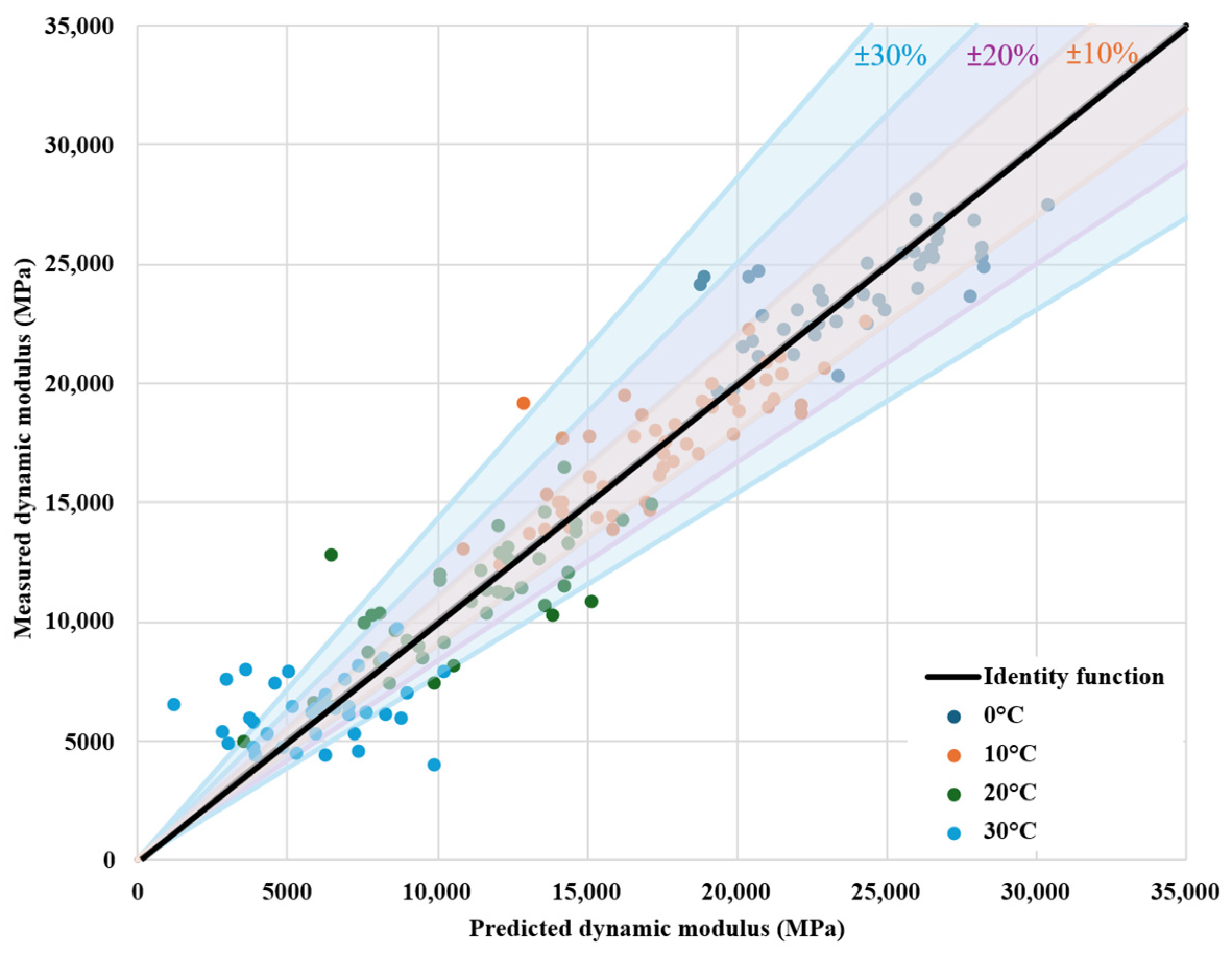
The relationship between the measured values of the dynamic modulus versus the calculated values of the predicted formula is plotted in Figure 5. Shading bands, corresponding to ±10%, ±20%, and ±30% deviation ranges from perfect predictions, are used to express the margin of error relative to perfect prediction. The majority of the data align well with the identity (perfect prediction) line, though some spread indicates higher prediction errors—especially at 30 °C. This implies broader variability in the modulus, which amplifies prediction errors, likely due to binder recovery, confirming previous results. In contrast, at low temperatures, the spread is narrower, so even a modestly accurate linear fit produces relatively small residual errors.

3.4. Sigmoidal Dynamic Modulus Prediction Model

The sigmoidal model is a mathematical model that describes the viscoelastic stiffness of asphalt mixtures by modelling the relationship between the dynamic modulus and the reduced loading frequency by fitting the measured dynamic modulus data into a continuous, smooth S-shaped curve. This curve is called the master curve [32]. It is calculated as follows:

$$\log \left|E^{\mathrm{*}}\right|=\mathrm{ }\delta +{\displaystyle \frac{\alpha }{1+\exp \left(\beta +\gamma \log f_r\right)}}$$

(16)

where $\left|E^{*}\right|$ is the dynamic modulus (MPa); α, β, γ, and δ are regression parameters: α denotes the difference between the maximum and minimum logarithmic values of the dynamic modulus (MPa), β and γ are shape-fitting parameters controlling the horizontal shift and slope of the sigmoidal curve, respectively, and δ represents the logarithm of the minimum dynamic modulus; and $f_r$ is the reduced frequency (Hz).

The latter is defined as follows:

$$f_r=a_T\times f\mathrm{ }\leftrightarrow \log f_r=\log a_T+\log f$$

(17)

where f is the tested frequency at the temperature T (Hz), T is the tested temperature (°C), and $a_T$ is the time–temperature shift factor. The shift factor is estimated using an empirical model.

The optimal model parameters were calibrated using Microsoft Excel’s Solver add-in by minimizing the error between the measured and predicted dynamic modulus (|E*|) values. The same dataset, used in the previous prediction model, was studied for the sigmoidal model.

To assess the performance of the sigmoidal prediction model to predict the dynamic modulus of asphalt mixtures, standard regression metrics were calculated at each temperature condition, as well as for all datasets combined.

Table 8. Regression analysis of the sigmoidal model.

	R2	RMSE	MAE	MAPE (%)
0 °C	0.962	747.73	498.17	2.25
10 °C	0.977	602.19	389.08	2.61
20 °C	0.982	509.34	283.23	3.47
30 °C	0.987	306.26	166.00	3.71
All Data	0.994	568.44	337.16	3.00

summarizes the model’s performance using the coefficient of determination (R²), root mean square error (RMSE), mean absolute error (MAE), and mean absolute percentage error (MAPE). The results indicate a high level of accuracy between the measured and predicted values, with R² values higher than 0.96. In addition, the consistently low MAPE values (<4%) at all temperatures highlight the model’s strong predictive capability and minimal relative error.

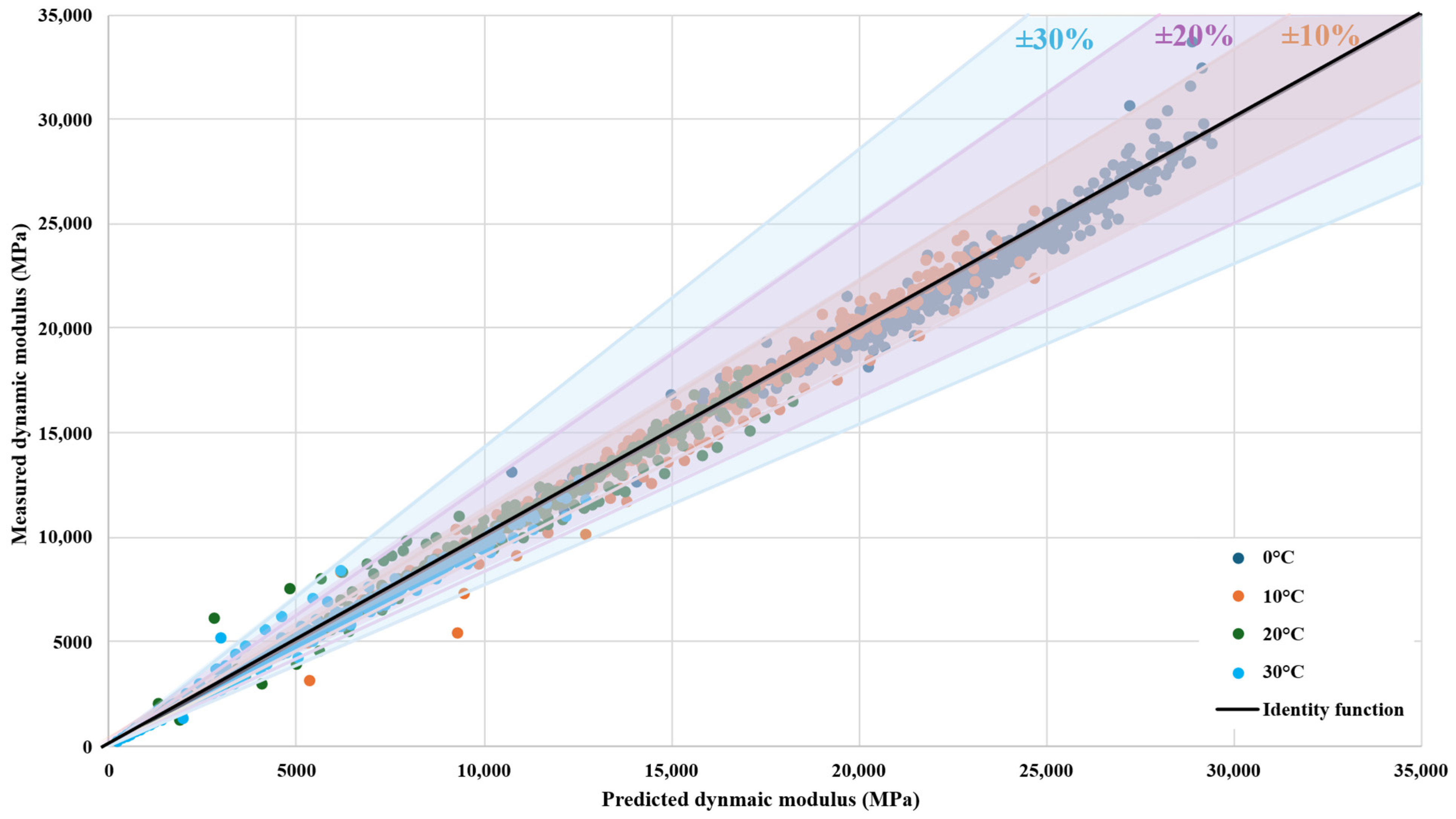
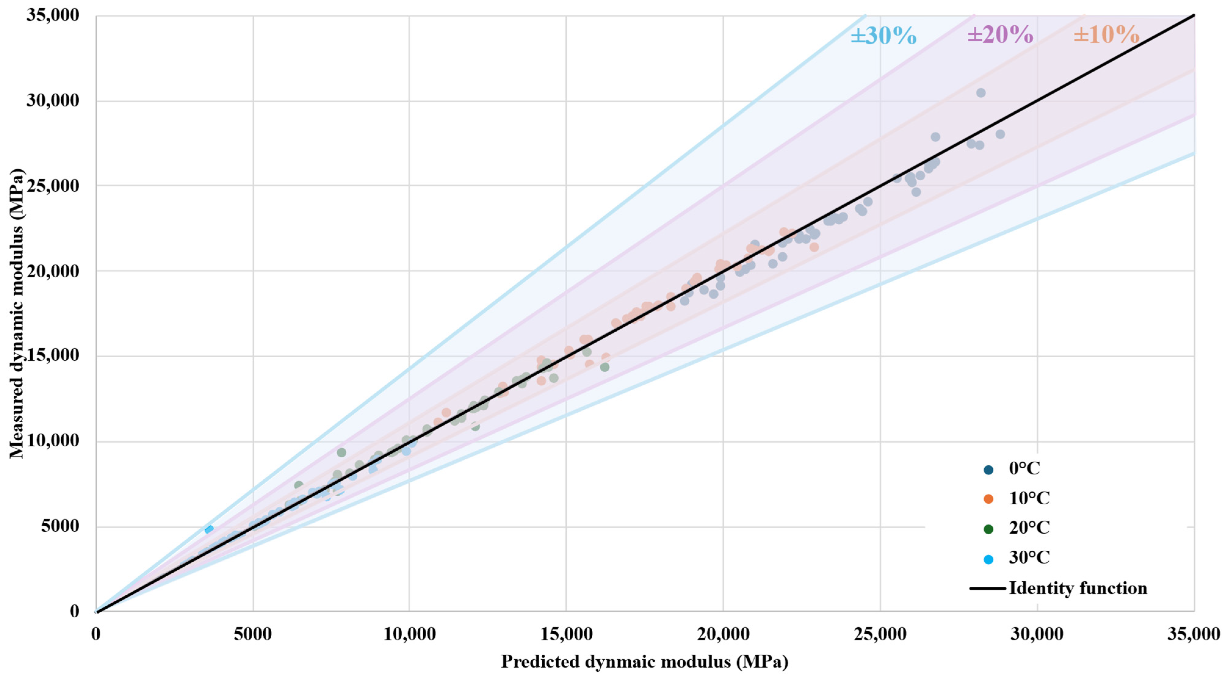
Figure 6 and Figure 7 present a comparison between predicted and measured dynamic modulus values using the sigmoidal model for asphalt mixtures tested at 0 °C, 10 °C, 20 °C, and 30 °C across various loading frequencies (0.1–50 Hz) and at 10 Hz, respectively. The data points are color-coded by temperature and plotted against the identity line (x = y), which represents perfect prediction. Additionally, three accuracy bands are included to illustrate deviations of ±10%, ±20%, and ±30% from the measured values.

The majority of the data points are scattered within the ±10% range, and a slight portion lies within the ±20% deviation band, demonstrating the model’s good prediction accuracy across different conditions. A limited number of data fall within the ±30% deviation band and beyond, mostly at high temperatures and low modulus values.

Overall, these results indicate that the sigmoidal model is effective in capturing the viscoelastic response of asphalt mixtures under a wide range of loading and thermal conditions. It provides a reliable and interpretable approach for dynamic modulus prediction.

4. Conclusions

This study compared the performance of two predictive models—the GRA-MLR model and sigmoidal model—to estimate the dynamic modulus (|E*|) of asphalt mixtures. While the GRA-MLR model was effective in identifying the relative influence of material factors, its predictive accuracy was moderate, with modest R² values ranging from 0.4743 to 0.6547. This indicates that the model can capture only a part of the variability in dynamic modulus.

On the other hand, the sigmoidal prediction model exhibited superior performance compared to that of the GRA-MLR model, achieving coefficients of determination above 0.96 at all temperature conditions. The root mean square error (RMSE) and mean absolute error (MAE) were also significantly low, with most predictions falling within ±10% to ±20% deviation from measured values.

This study also revealed that, at lower temperatures (0 °C and 10 °C), the model’s predictions were primarily governed by the static stiffness modulus and gradation characteristics, whereas as temperatures increased to 20 °C and 30 °C, reclaimed asphalt (RA) contents became increasingly significant, proving a temperature-dependent shift in variable influence. This shift suggests that aged binder recovery plays a more prominent role in mixture stiffness under warmer conditions. This conclusion was also reflected in both the regression analysis and the prediction error trends at 30 °C.

Despite its limitations in accuracy, the GRA-MLR model remains valuable due to its simplicity and capability for variable interpretation, especially at low temperatures. In contrast, the sigmoidal model delivers better predictive accuracy and robustness, requiring more comprehensive experimental data and potentially longer testing times, which can increase costs and complexity.

In summary, in scenarios where predictive accuracy is supreme and sufficient data and computational resources are available, the sigmoidal model is the preferred tool in detailed design applications. In contrast, the GRA-MLR model offers practical benefits in resource-limited contexts by facilitating rapid assessments and providing interpretability through its identification of key influencing variables, even though this model demonstrated less precise prediction performance. A combined modeling strategy—using GRA-MLR for preliminary variable screening and the sigmoidal model for refined analysis—can effectively balance computational efficiency with predictive rigor, enhancing decision-making in mechanistic–empirical pavement design.

References

1. Su, N.; Xiao, F.; Wang, J.; Amirkhanian, S. Characterizations of base and subbase layers for Mechanistic-Empirical Pavement Design. Constr. Build. Mater. 2017, 152, 731–745. [Google Scholar] [CrossRef]
2. Bi, Y.; Guo, F.; Zhang, J.; Pei, J.; Li, R. Correlation analysis between asphalt binder/asphalt mastic properties and dynamic modulus of asphalt mixture. Constr. Build. Mater. 2021, 276, 122256. [Google Scholar] [CrossRef]
3. Zhao, Z.; Xiao, F.; Toraldo, E.; Crispino, M.; Ketabdari, M. Effect of crumb rubber and reclaimed asphalt pavement on viscoelastic property of asphalt mixture. J. Clean. Prod. 2023, 428, 139422. [Google Scholar] [CrossRef]
4. Zeiada, W.; Obaid, L.; El-Badawy, S.; El-Hakim, R.A.; Awed, A. Benchmarking Classical and Deep Machine Learning Models for Predicting Hot Mix Asphalt Dynamic Modulus. Civ. Eng. J. 2025, 11, 76–106. [Google Scholar] [CrossRef]
5. Singh, D.; Zaman, M.; Commuri, S. Artificial Neural Network Modeling for Dynamic Modulus of Hot Mix Asphalt Using Aggregate Shape Properties. Am. Soc. Civ. Eng. 2013, 25, 54–62. [Google Scholar] [CrossRef]
6. Rahman, A.; Tarefder, R.A. Dynamic modulus and phase angle of warm-mix versus hot-mix asphalt. Constr. Build. Mater. 2016, 126, 434–441. [Google Scholar] [CrossRef]
7. Basnet, K.S.; Shrestha, J.K.; Shrestha, R.N. Pavement performance model for road maintenance and repair planning: A review of predictive techniques. Digit. Transp. Saf. 2023, 2, 253–267. [Google Scholar] [CrossRef]
8. Jweihan, Y.S.; Al-Kheetan, M.J.; Rabi, M. Empirical Model for the Retained Stability Index of Asphalt Mixtures Using Hybrid Machine Learning Approach. Apploed Syst. Innov. 2023, 6, 93. [Google Scholar] [CrossRef]
9. Abdelaziz, N.; El-Hakim, R.; El-Badawy, S.M.; Afify, H.A. International Roughness Index prediction model for flexible pavements. Int. J. Pavement Eng. 2020, 21, 88–99. [Google Scholar] [CrossRef]
10. Pérez-Acebo, H.; Mindra, N.; Railean, A.; Rojí, E. Rigid pavement performance models by means of Markov Chains with half-year step time. Int. J. Pavement Eng. 2019, 20, 830–843. [Google Scholar] [CrossRef]
11. Witczak, M. Simple Performance Test for Superpave Mix Design; NCHRP Report 465; Transportation Research Board: Washington, DC, USA, 2002. [Google Scholar]
12. Al-Khateeb, G.; Shenoy, A.; Gibson, N.; Harman, T. A new simplistic model for dynamic modulus predictions of asphalt paving mixtures. J. Assoc. Asph. Paving Technol. 2006, 75, 1254–1293. [Google Scholar]
13. Christensen, D.W., Jr.; Pellinen, T.; Bonaquist, R.F. Hirsch model for estimating the modulus of asphalt concrete. J. Assoc. Asph. Paving Technol. 2003, 72, 97–121. [Google Scholar]
14. Zhang, M.; Zhao, H.; Fan, L.; Yi, J. Dynamic modulus prediction model and analysis of factors influencing asphalt mixtures using gray relational analysis methods. J. Mater. Res. Technol. 2022, 19, 1312–1321. [Google Scholar] [CrossRef]
15. Shu, X.; Huang, B. Micromechanics-based dynamic modulus prediction of polymeric asphalt concrete mixtures. Compos. Part B Eng. 2008, 39, 704–713. [Google Scholar] [CrossRef]
16. Zheng, C.; Li, R.; Hu, M.; Zou, L. Determination of low-temperature crack control parameter of binding asphalt materials based on gray correlation analysis. Constr. Build. Mater. 2019, 217, 226–233. [Google Scholar] [CrossRef]
17. Chen, Q.; Wang, C.; Wen, P.; Sun, X.; Guo, T. Performance evaluation of tourmaline modified asphalt mixture based on grey target decision method. Constr. Build. Mater. 2019, 205, 137–147. [Google Scholar] [CrossRef]
18. EN 14023; Bitumen and Bituminous Binders-Specification Framework for Polymer Modified Bitumens. European Committee for Standardization: Brussels, Belgium, 2010.
19. EN 12591; Bitumen and Bituminous Binders—Specifications for Paving Grade Bitumens. European Committee for Standardization: Brussels, Belgium, 2011.
20. ČSN 65 7222-1; Bitumen and Bituminous Binders-Modified Asphalts for Road Construction-Part 1: Polymer Modified Asphalts (Asfalty a Asfaltová Pojiva-Silniční Modifikované Asfalty-Část 1: Polymerem Modifikované Asfalty). Český normalizační institute (ČNI): Prague, Czech Republic, 2017.
21. Yin, F.; Kaseer, F.; Arámbula-Mercado, E.; Epps Martin, A. Characterising the long-term rejuvenating effectiveness of recycling agents on asphalt blends and mixtures with high RAP and RAS contents. Road Mater. Pavement Des. 2017, 18, 273–292. [Google Scholar] [CrossRef]
22. Al-Saffar, Z.H.; Yaacob, H.; Satar, M.; Saleem, M.K.; Lai, J.C.; Putra Jaya, R. A review on rejuvenating materials used with reclaimed hot mix asphalt. Can. J. Civ. Eng. 2021, 48, 233–249. [Google Scholar] [CrossRef]
23. Abduljabbar, N.; Al-Busaltan, S.; Dulaimi, A.; Al-Yasari, R.; Sadique, M.; Al Nageim, H. The effect of waste low-density polyethylene on the mechanical properties of thin asphalt overlay. Constr. Build. Mater. 2022, 315, 125722. [Google Scholar] [CrossRef]
24. Lubis, A.S.; Muis, Z.A.; Siregar, N.A. The effects of low-density polyethylene (LDPE) addition to the characteristics of asphalt mixture. IOP Conf. Ser. Earth Environ. Sci. 2020, 476, 012063. [Google Scholar] [CrossRef]
25. Picado-Santos, L.G.; Capitão, S.D.; Neves, J.M.C. Crumb rubber asphalt mixtures: A literature review. Constr. Build. Mater. 2022, 247, 118577. [Google Scholar] [CrossRef]
26. Xiang, L.; Cheng, J.; Que, G. Microstructure and performance of crumb rubber modified asphalt. Constr. Build. Mater. 2009, 23, 3586–3590. [Google Scholar] [CrossRef]
27. Adepu, R.; Ramayya, V.V.; Mamatha, A.; Ram, V.V. Fracture studies on basalt fiber reinforced asphalt mixtures with reclaimed asphalt pavement derived aggregates and warm mix additives. Constr. Build. Mater. 2023, 386, 131548. [Google Scholar] [CrossRef]
28. ČSN 73 6121; Road Building—Asphalt Pavement Courses—Construction and Conformity Assessment. Office for Technical Standardization, Metrology and State Testing (Úřad pro Technickou Normalizaci, Metrologii a Státní Zkušebnictví): Prague, Czech Republic, 2023.
29. EN 12697-30; Bituminous Mixtures—Test Methods—Part 30: Specimen Preparation by Impact Compactor. European Committee for Standardization: Brussels, Belgium, 2018.
30. EN 12697-33; Bituminous Mixtures—Test Method—Part 33: Specimen Prepared by Roller Compactor. European Committee for Standardization: Brussels, Belgium, 2019.
31. EN 12697-26; Bituminous Mixtures—Test Methods for Hot Mix. European Committee for Standardization: Brussels, Belgium, 2012.
32. Garcia, G.; Thompson, M. HMA Dynamic Modulus Predictive Models (a Review). FHWA-ICT-07-005. 2007. Available online: https://www.ideals.illinois.edu/items/46018 (accessed on 7 September 2025).
Figure 1. Specimen preparation procedure.
Infrastructures 10 00269 g001
Figure 2. Methodology flowchart: three major steps, starting with data preparation, followed by sensitivity analysis and, finally, prediction processes.
Infrastructures 10 00269 g002
Figure 3. Sensitivity analysis of grey relational grades under different ζ values for key mixture factors.
Infrastructures 10 00269 g003
Figure 4. Grey relational grades distributions at each temperature ((a) at 0 °C, (b) at 10 °C, (c) at 20 °C, and (d) at 30 °C).
Infrastructures 10 00269 g004
Figure 5. Measured |E*| versus predicted |E*| for different asphalt mixtures at different testing temperatures (0 °C, 10 °C, 20 °C, and 30 °C) and frequencies (50, 30, 20, 15, 10, 8, 5, 3, 2, 1, and 0.1 Hz) (shaded bands correspond to ±10% (orange), ±20% (purple), and ±30% (blue) deviation ranges from perfect predictions).
Infrastructures 10 00269 g005
Figure 6. Measured |E*| versus predicted |E*| for different asphalt mixtures at different testing temperatures (0 °C, 10 °C, 20 °C, and 30 °C) and frequencies (0.1, 1, 2, 3, 5, 8, 10, 15, 20, 30, and 50 Hz) (shaded bands correspond to ±10% (orange), ±20% (purple), and ±30% (blue) deviation ranges from perfect predictions).
Infrastructures 10 00269 g006
Figure 7. Measured |E*| versus predicted |E*| for different asphalt mixtures at different testing temperatures (0 °C, 10 °C, 20 °C, and 30 °C) at 10 Hz (shaded bands correspond to ±10% (orange), ±20% (purple), and ±30% (blue) deviation ranges from perfect predictions).
Infrastructures 10 00269 g007