Structural Stability of Cycle Paths—Introducing Cycle Path Deflection Bowl Parameters from FWD Measurements

Abstract

A recurrent challenge on cycle paths are edge cracks, which affect the traffic safety and accessibility of cyclists and produce high maintenance costs. Being both structurally thinner and narrower structures than roads, the cycle paths are extra prone to this problem. A few passages of heavy vehicles in unfavourable conditions might be enough to break the edge. The load-bearing capacity of eight municipal cycle paths in Linköping, Sweden, were assessed by falling weight deflectometer (FWD) and light falling weight deflectometer (LWD) measurements during a year-long cycle. A set of alternative Deflection Bowl Parameters (DBPs), better adapted to the structural design of cycle paths, were suggested and evaluated. The results of the FWD measurements showed that these suggested DBPs are a promising approach to evaluate the load-bearing capacity of cycle paths. From the results of the LWD measurements, it was found that the load-bearing capacity varies considerably with lateral position. The conclusion is that it might be more fruitful to measure the load-bearing capacity by LWD close to the edge, rather than the traditional approach of FWD measurements along the centre line of the cycle path.

1. Introduction

A recurrent challenge on cycle paths is the presence of edge cracks or edge deformations [1,2], which apart from posing a traffic safety issue for the cyclists [3,4], diminishes the effective width of the cycle path, thus also causing a lack of accessibility for the cyclists [5,6]. From an asset management perspective, the formation of edge cracks and deformations contributes to higher maintenance costs, as patching and reinforcements are generally needed to address the problem [7]. If unattended, the cracks risk further accelerating the degradation process as water seeps into the structure, weakening the structural stability of the unbound granular layers (UGLs) [8]. The cause of the edge cracks is mainly due to the transiting of heavy vehicles close to the pavement edge [9]. There are several vehicle-related factors that affect the impact on the structure from the traffic loads, such as the number of passings, and load magnitude and distribution, along with characteristics of the tires, i.e., dimension, tire pressure, and tire pattern [7]. These factors are not necessarily known for a specific cycle path [1], as it is not common for the cycle path operators to monitor it. The maintenance is often conducted by separate contractors, and there could be other heavy vehicles present, apart from the planned operation and maintenance activities. For example, a study from Paris suggests that more than 60 percent of the surveyed delivery operations were made with an illegally parked vehicle, i.e., on a bus or bicycle lane or on the sidewalk [10]. The characteristics of cycle paths, which are generally thinner and narrower structures than most roads, in combination with an often poor drainage and low speeds the vehicles, make them extra prone to this type of distress. There are also other highly important structural factors that affect the degradation rate, such as the geometric effect of side slopes which creates a lack of lateral support to the UGLs, material properties of the aggregates, and the degree of compaction of the UGLs [11]. Therefore, it is important to investigate the load-bearing capacity of cycle paths, especially when it is at its minimum, i.e., during the thawing period.

A common way to investigate the load-bearing capacity of pavement structures is by a falling weight deflectometer (FWD) [12]. An advantage of this non-destructive evaluation method is that weaknesses in different parts of the structure can be identified. If the structural layer thicknesses are known, the measured deflections can be compared to calculated deflections by iterative back calculations by assuming the Elastic moduli (E), i.e., a measure of the load-bearing capacity for those structural layers [13]. However, the general model which is used in Sweden for the back calculation of FWD measurements does not apply for thin-surfaced asphalt pavements (TSAP), as it assumes an asphalt layer thickness of at least 75 mm [14]. This is due to the assumption of the linear elastic behaviour of the structure, where the asphalt concrete (AC) thickness should be at least half of the loading plate radius [13]. For the TSAP, however, it is rather believed that there is a significant portion of non-linearity in the behaviour [11].

There is interest in establishing better design principles for the construction of cycle paths [15,16,17]. As mentioned, one way to assess structural stability is by FWD measurements. An advantage of the FWD is that it simulates a passing heavy vehicle at highway speed. However, a disadvantage is that due to its size, the measurements cannot be conducted close to the pavement edge. An alternative approach is to use a light falling weight deflectometer (LWD), which could be placed closer to the edge. Low weight, portability, and easy handling, along with the low cost of the equipment, are other advantages of the LWD [18]. Kestler et al. [19] found a strong correlation (R² = 0.87) between deflection measurements from an LWD and FWD on thin (≤125 mm) asphalt pavements. Other studies, e.g., Refs. [20,21] have also found relatively strong correlations (R² = 0.62 and 0.64, respectively) between the FWD and some deflection basin parameters (DBPs), and it has thus been suggested that the LWD could be used instead of the FWD when assessing the structural capacity of thin pavement structures [18].

In short, a more optimal approach for load-bearing capacity investigations on cycle paths is needed. The purpose of this paper is to propose the outlines for such a procedure by first investigating how the load-bearing capacity varies with different conditions such as age, structural and geometrical design, lateral position, material properties, and climatic conditions in terms of temperature and moisture to pinpoint critical situations. This is performed through FWD measurements during a year-long cycle, which are complemented by LWD measurements and transverse surface profile measurements. Due to the described difficulty with the normal procedures of back calculations, an alternative set of DBPs that are better adapted to the structural design of cycle paths is proposed and evaluated.

2. Materials and Methods

For the investigation of load-bearing capacity, eight structurally different cycle paths in Linköping, Sweden, were measured with FWD and LWD. The FWD measurements were conducted during a one-year cycle, starting in December 2022. The LWD measurements were conducted between November 2023 and March 2024. Measurements of the transversal surface evenness were also conducted with the Primal profile instrument [22] on 8 December 2023.

2.1. Selected Cycle Paths

The eight municipal cycle paths in the study were chosen in collaboration with Linköping municipality to obtain a variety of cycle path structures with regard to structural design, age, function, and specific conditions due to their location in the terrain, as described in

Table 1. Relevant properties for the investigated cycle paths.

Cycle Path	Datalinjen	Hertig Johans Allé	Lambohovsleden	Olaus Magnus Väg	Rydsvägen	Stratomtavägen	Universitetsfältet	Universitetsvägen
Age (years)	27	9	8	28	3	28	24	21
Width (m)	3.1	3.4	4	2.9	4	2.8	3	3.8
Wearing course (mm)	30	40	40	30	45	20	30	35
Bound base course (mm)	-	-	-	-	-	50	-	-
Base course (mm)	120	120	80	120	80	130	120	120
Subbase (mm)	250	340	340	250	375	100	350	390
Total thickness (mm)	400	500	460	400	500	300	500	545
Mix, wearing course 1	80 MAB 8 T	ABT11	ABT11 160/220	80 MAB 12 T	ABT11 160/220	80 MAB 8 T	ABT11 180	-
Mix, base course 2	-	-	-	-	-	AG	-	-
Material, base course 3	Natural gravel	Crushed rock	Crushed rock	Natural gravel	Crushed rock	Natural gravel	Crushed rock	Natural gravel
Material, subbase 4	Natural gravel	Crushed rock	Crushed rock	Natural gravel	Crushed rock	Natural gravel	Crushed rock	Natural gravel
Soil type	Clay	Clay	Rock, sandy till	Clay	Fine sand	Fine sand	Clay	Clay
Permeability	Low	Low	Medium	Low	High	High	Low	Low
Drainage pipe Ø (mm) 5	-	110	2 × 110	-	110	-	-	110
Cross fall (%)	1.0	3.6	2.3	1.2	1.3	3.0	0.4	1.7
Side slope inclination	-	1:10	1:3	-	1:3	1:5	1:6	1:2
Sweep-salted	Yes	No	Yes	No	Yes	Yes	No	Yes

¹ 80 MAB 8 T and 80 MAB 12 T are dense-graded AC with a pen grade of 160/220, along with a maximum aggregate size of less than 8 mm and 12 mm, respectively. ABT11 160/220 and ABT11 180 indicate a dense-graded AC with a pen grade of 160/220. ² AG is a dense-graded AC, normally with a maximum aggregate size of 16 or 32 mm, which is applied to enhance the load-bearing capacity. ³ Properties are not known but according to the Swedish design standard a well-graded unbound granular material (UGM) with a maximum nominal aggregate size of 32 mm, maximum fine content ≤ 5%, M_DE ≤ 25, is to be used for both natural gravel and crushed rock. ⁴ Properties are not known but normally a well-graded UGM with a maximum nominal aggregate size of 100 mm, maximum fine content ≤ 5%, M_DE ≤ 20, and at least suffice the criterion for LA₄₀ to be used for both natural gravel and crushed rock. ⁵ “Drainage pipe” indicates the diameter of longitudinal plastic pipes, installed 300 mm below the SG surface.

. The cycle paths are located so closely that they could all be measured during the same day (Figure 1a), which assured frost and weather conditions that were as equal as possible for the measurements. The maps of The Geological Survey of Sweden (SGU) have been consulted for the properties of the subgrade (SG) (Figure 1b). These maps present geological information, such as permeability and soil types, down to a resolution of 1:1250, which was deemed to be sufficient for the purpose of this study.

Figure 2 presents images of the cycle paths. Their structural designs and drainage properties, as stated in the construction plans of Linköping municipality, are found in Table 1. According to the municipality, none of the cycle paths have had any resurfacing of the AC since construction. Apart from Datalinjen, which has a longitudinal crack going along the bottom of the rut at the left-hand side of the cycle path (which can be seen as a strip of water to the left in Figure 2a), only minor distress is present on the cycle path surfaces. For example, at Hertig Johans allé in Figure 2c, a thin longitudinal crack along the right-hand edge is visible. Even though this is not a serious distress, it could be an indication that the load-bearing capacity is insufficient. As can be seen to the left in the image in Figure 2g, there is standing water on Universitetsfältet due to the unevenness of the surface. This is related to an insufficient cross fall (0.4%), which is well below the recommended 1–2 percent of the Swedish geometrical design standard [23].

As Table 1 shows, there are considerable differences in the properties between the different cycle path structures. The age, which ranges from 3 to 28 years, affects the accumulated degradation effects, such as plastic deformations or the aging of the bitumen. Aging potentially increases the stiffness as the bitumen hardens, but at the same time it makes the AC more brittle and prone to cracking [24]. In all, higher age will therefore likely have negative effects on the structure’s load-bearing capacity. The narrow widths of the cycle paths, which range from 2.8 to 4 m, diminish the possible spread in the transiting heavy vehicles’ lateral positions, which influences the degradation rate of the structures [25,26,27]. The thicknesses of the constituent structural layers are important as the materials used for each layer differ in load-bearing capacity, ranging from the strongest materials, i.e., the AC, at the surface, down to the weakest material in the SG. At the surface, the structure will be subjected to more concentrated loads, i.e., higher stress, compared to deeper down in the structure where the load is distributed onto a larger surface, i.e., lower stress [28]. Consequently, a thin AC layer does not distribute the load onto the UGLs as much as a thicker AC. The choice of material for the UGLs is also important, as crushed rock shows better load-bearing capacities than natural gravel due to a higher internal friction angle of the less rounded shape of the aggregates [7]. There are other characteristics of the material which also affect the load-bearing capacity, such as the grain size distribution, maximum grain size, content of fines, and mineralogy [11]. Since these factors are unknown in this study, the effects of these parameters were omitted in the analysis. The soil type of the SG is related to permeability, which affects the drainage rate of the structure. For some of the structures, additional longitudinal pipes are installed in a grave of permeable granular material to facilitate the drainage. A higher cross fall of the cycle path surface and steeper side slopes contribute to a better water runoff. The winter maintenance method called “sweep-salting”—which consists of a maintenance vehicle sweeping loose snow off the surface and subsequently applying salt to maintain a bare surface [29]—is applied on some of the cycle paths. The rest are treated with conventional ploughing and gritting, e.g., Olaus Magnus väg in Figure 2d. This is an important aspect to consider as the different winter maintenance methods affect the number of passings by maintenance vehicles—sweep-salting usually requires more frequent actions. It has been suggested that the sweep-salting method might accelerate the rate of degradation of the cycle paths [30].

2.2. Equipment

Measurements were conducted with an FWD, see Figure 3a, at 19 different occasions during a one-year period from 8 December 2022 to 8 November 2023. Between 8 November 2023 and 3 March 2024, measurements were also conducted on 5 occasions with an LWD, see Figure 3b. In addition, the transverse profiles of the section where the LWD measurements were conducted for each cycle path were measured using the Primal longitudinal profile instrument [22], see Figure 3c. For the LWD, only the deflection in the centre of the loading plate (D₀) was measured.

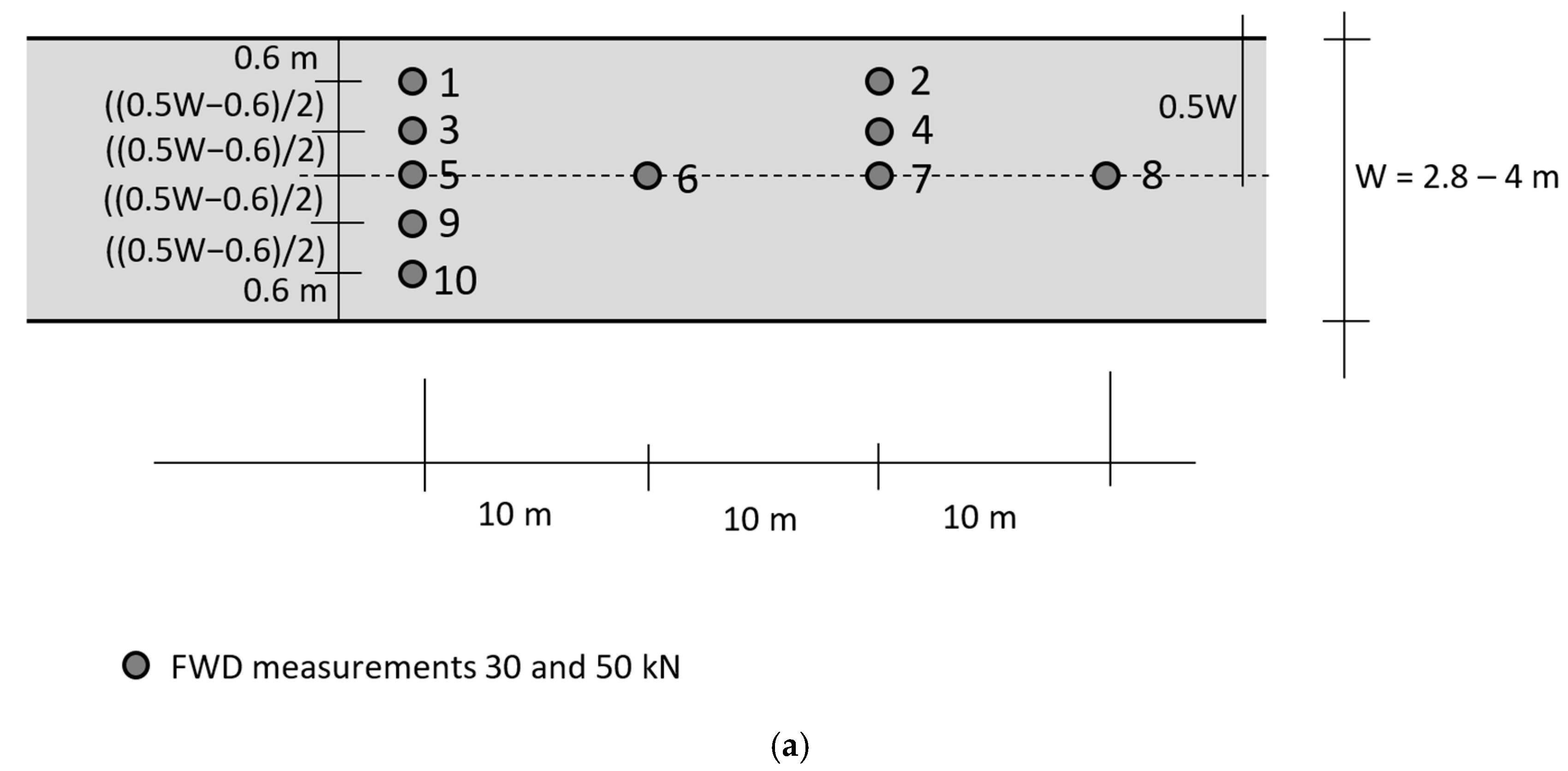
2.3. Measurements and Measuring Procedure

The FWD measurements were conducted following a scheme consisting of 10 measuring points on each cycle path, forming a mesh according to Figure 4a, where the numbers (1–10) indicate the measuring sequence. The closest position to the pavement edge that was possible for the FWD measurement was 0.6 m. The LWD measurements started in the first longitudinal section, with the edge of the loading plate converging with the cycle path edge. The plate was then moved to the adjacent position, on the same section, in such a way that the plate positions never overlapped (except from the last measuring point for each cycle path) according to the illustration in Figure 4b.

For each FWD measuring point, three induced load impulses of 30 kN were applied, which were then followed by three load impulses of 50 kN, generating contact pressures of 424 and 707 kPa, respectively. The FWD registered the exact load, air temperature, and surface temperature, along with the deflection in each geophone for each of the load impulses.

The FWD measurements were conducted according to TRV’s guidelines [14], with the adaptation of the norms to suit the 30 kN loads as well. The guideline establishes that the applied load should be 50 kN and the deflection sensors should be placed at the centre of the loading plate (D₀), and consecutively at the distances 200 mm (D₂₀₀), 300 mm (D₃₀₀), 450 mm (D₄₅₀), 600 mm (D₆₀₀), 900 mm (D₉₀₀), and 1200 mm (D₁₂₀₀) from the centre. A five percent deviation from the 50 kN load is admissible, and the measured deflections should be adjusted with a correctional factor, consisting of the quota between the actual applied load and a 50 kN load. A certain repacking of the material in the UGLs takes place with each load impulse, which is why the result from the second or possibly third load impulse is normally used for calculations of the load-bearing capacity. A maximum of five percent deviation between load impulses is allowed, otherwise the next load impulse should be used. Apart from the deflections, the FWD should also measure air and pavement temperatures [14]. The measured deflections are normally adjusted to represent deflections at 10 °C; that is however omitted for this study, assuming that the temperature’s effect on the load-bearing capacity is negligible for such thin AC layers, as has been previously suggested [31,32].

The measurement routine for the LWD measurements consists of three preloading load impulses, where the values are not recorded, followed by three measuring load impulses. The magnitude of the load impulses is 7.07 kN, generating a contact pressure of 100 kPa. As only D₀ is measured with the LWD, the load being 7.07 kN, and air and surface temperature not being detected, the guidelines are not relevant for LWD measurements. However, the maximum five percent deviation between load impulses criterion was applied for the LWD measurements as well.

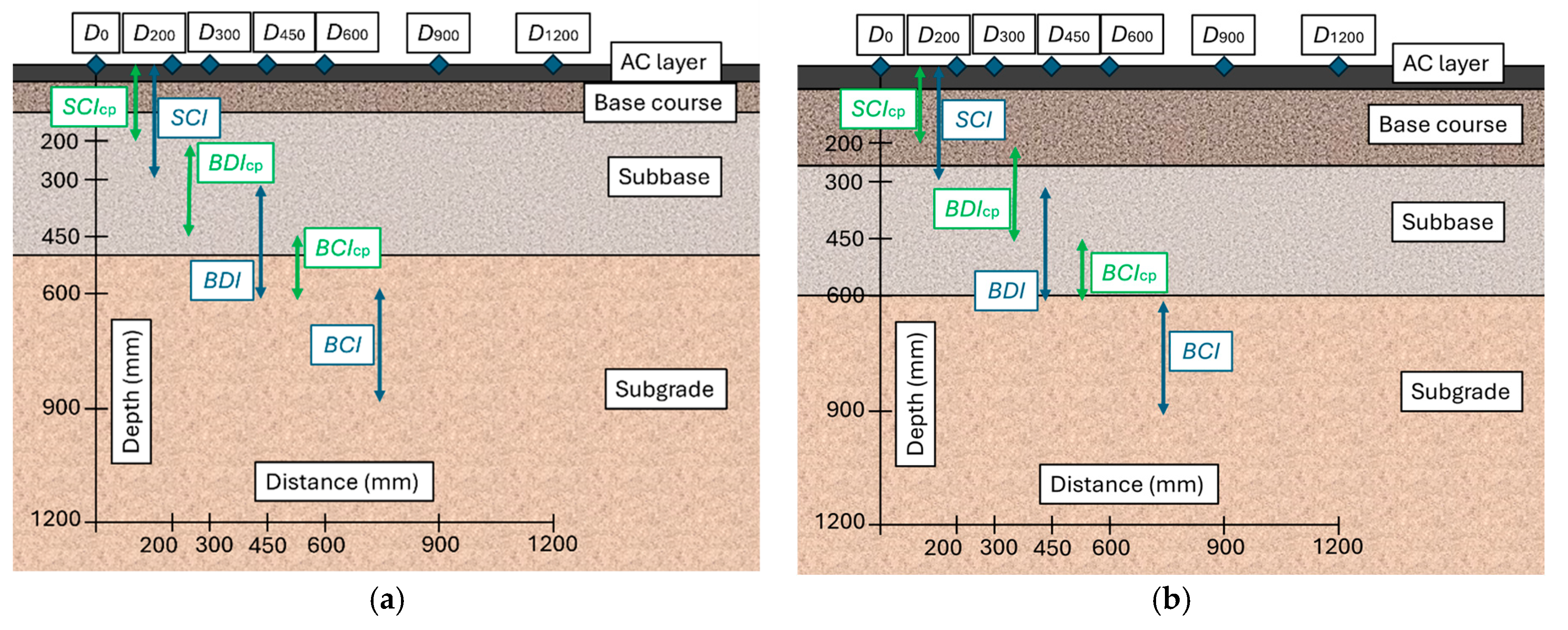
2.4. Data Analysis and Metrics

The guidelines stipulate that the thickness of the AC should be at least 75 mm thick for back calculations, which in practice disqualifies basically all cycle path structures. If the thickness of an unbound layer is less than 100 mm, it should be added to the underlaying layer and treated as one homogenous layer. This would also be the general case for cycle path structures in Sweden, where a standard unbound base course (BC) is only 80 mm thick [33]. The lowest layer in the calculation model is the SG, which has a significant impact on the resilient modulus of the calculated structure. The SG is stated to contribute about 70 percent of the D₀ for FWD measurements [34]. In the model, the SG should be represented as a homogenous layer which rests on top of a rigid layer three metres below the surface [14]. For Lambohovsleden, it is suspected that there is solid rock closer to the pavement surface than these three metres.

If the back calculation of E for the constituent layers of the structure renders values that are to be considered unrealistic according to specified values in the Swedish guidelines [14], or in the case that the calculated deflections are not coherent with the measured ones, the result should be discarded.

Another approach to evaluate the load-bearing capacity of pavement structures is to use parameters which describe the characteristics of the deflection bowl that is formed from the FWD load impulse. One set of such DBPs, which relates the deflections measured at some of the geophones of the FWD, are Surface Curvature Index (SCI), Base Damage Index (BDI), and Base Curvature Index (BCI). They sometimes also go under the alternative names Base Layer Index (BLI), Middle Layer Index (MLI), and Lower Layer Index (LLI) [34]. These DBPs have been calculated from the deflections measured with the 50 kN FWD along the centre line of the cycle paths. It should be noted that the BDI and BCI in the Swedish guidelines [14] are inversely defined from how these denotations are used in the international literature, e.g., [35]. The international convention of these DBPs has been used for the purpose of this article to avoid misunderstandings. The SCI corresponds to the part of the total deflection that occurs in the upper parts of the structure, primarily the BC [36] and is calculated by Equation (1).

SCI = D₀ − D₃₀₀

(1)

The BDI indicates the stability of the middle part of the structure, i.e., the SB [36] and is calculated by Equation (2).

BDI = D₃₀₀ − D₆₀₀

(2)

Finally, the BCI describes the stability of the lower parts of the structure, capping, and SG layers [36]. This calculation is conducted by Equation (3).

BCI = D₆₀₀ − D₉₀₀

(3)

These DBPs contribute to more diverse information about the structural stability of different parts of the structure than the D₀ alone. Yet, they are still easy and straightforward to calculate. Thus, they have been suggested as a smooth way of identifying structural weaknesses along a stretch of road, with the advantage of analyzing the structural layers that may need attention. Horak and Emery [34] describe how these DBPs are applied, with a three-grade rating (Sound, Warning and Severe) which is based on limit values for each DBP. The limit values assume a flexible pavement, designed for 3 × 10⁶ standard 80 kN axle loads.

Apart from having thin AC layers, cycle paths also generally have thin BC, and even thin SB, compared to those of most roadways. In the Swedish structural design manual [33], cycle paths are to be designed for 1.5 × 10⁵ standard single axle loads of 100 kN. By the fourth power law, that equals some 3.66 × 10⁵ 80 kN standard axles. Consequently, these limit values need to be adjusted to suit cycle path conditions. However, it has been shown that the fourth power law is not valid for TSAP [37]. This means that the calculated number of equivalent passings may not be correct, which in turn means that the adjusted limit values are afflicted with uncertainties. Even so, converting a certain number of passings with 100 kN axle loads into 80 kN axle loads should imply more passings, and for lack of a better estimate this approach is still chosen for the purpose of this study. Maree and Bellekens [38] created a chart through which such a conversion can be conducted. The estimated adjusted limit values are presented along with the original limit values [34] in

Table 2. Limit values for the Deflection Bowl Parameters as proposed by Horak and Emery [34] for flexible pavements, designed for 3 × 10⁶ standard 80 kN axles, and the estimated adjusted limit values for cycle paths constructed according to the Swedish structural design manual, designed for 1.5 × 10⁵ standard 100 kN axles [33].

Structural Condition Rating	Deflection Bowl Parameter Limit Values Horak and Emery, 2006 [34]
	D0 (µm)	BLI (µm)	MLI (µm)	LLI (µm)
Sound	<400	<200	<100	<55
Warning	400–750	200–500	100–200	55–100
Severe	>750	>500	>200	>100
Structural Condition Rating	Estimated Deflection Bowl Parameter Limit Values TRV, 2023 [33]
	D0 (µm)	SCI (µm)	BDI (µm)	BCI (µm)
Sound	<720	<420	<220	<130
Warning	720–1350	420–1050	220–440	130–235
Severe	>1350	>1050	>440	>235

.

Another DBP, described in TRV’s guidelines [14], is the average module, E_r, which describes the stiffness of the structure beneath a certain geophone, from the depth of r and downwards [13]. r is thus measured from the surface and equals the distance from the geophone in question to the centre of the loading plate [14]. E_r is calculated by Equation (4).

$$E_r={\displaystyle \frac{1000·(1-v^2)·{\sigma }_0·a^2}{r·D_r}}$$

(4)

where

$v$ is the Poisson’s ratio.

${\sigma }_0$ is the contact pressure beneath the loading plate, in MPa.

$a$ is the radius of the loading plate in mm.

$r$ is the distance between the geophone and the centre of the loading plate in mm.

$D_r$ is the deflection at the distance of $r$ from the centre of the loading plate in µm.

In the special case of E_r when r = 0, i.e., considering the deflection in the centre of the loading plate, D₀ is called the surface module and constitutes an average E for the whole structure, including the SG. It is calculated by Equation (5).

$$E_0={\displaystyle \frac{1000\ast f\ast \left(1-v^2\right)\ast {\sigma }_0\ast a^2}{D_0}}$$

(5)

where

$f$ is a correctional factor for the design of the loading plate, which is π/2 for a solid loading plate as in this case, and the rest of the parameters are the same as for Equation (4).

The SCI, BCI, and BDI could theoretically be adjusted in accordance with the principle described for the E_r, so that they better represent the layer thicknesses found in cycle path structures—rather than those found in roadways—by using data from some of the other available geophones. These adjusted metrics are henceforth denoted SCI_cp, BDI_cp, and BCI_cp, where the index _cp is for cycle paths. They are described by Equations (6)–(8).

SCI_cp = D₀ − D₂₀₀

(6)

BDI_cp = D₂₀₀ − D₄₅₀

(7)

BCI_cp = D₄₅₀ − D₆₀₀

(8)

It should be mentioned that there is already an established DBP, called the Curvature Function (CF) [39], that complies with the definition of SCI_cp, in Equation (6). Still, the denotation SCI_cp is proposed as part of a coherent system of DBPs adapted especially for cycle path conditions. Visual comparisons between the two sets of DBPs on a cycle path structure and a low-volume road structure are presented in Figure 5. As Figure 5a indicates, for typical cycle path layer thicknesses the proposed metrics (green arrows) better isolate the inherent layers, i.e., the BC, SB, and upper part of the SG, due to the shorter spans. For the layer thicknesses of the low-volume road, the established DBPs (blue arrows) show a better fit instead, due to the larger spans.

In the development of the SCI_cp, considerations have been taken into account to the fact that the results from the CF are deemed to give less accurate values than SCI due to the confounding effect of the small distance between the D₂₀₀ geophone and the edge of the loading plate, which has a radius of 150 mm [34]. However, this adjustment may still be justifiable for cycle paths, because the deflection sensors must be located closer to the load centre for pavements with thin asphalt layers than in the case of a thicker asphalt pavement [13].

An important aspect of the structural stability of cycle paths is the geometric effect of side slopes. The geometric factor (GEOM) [40] describes an average, structurally independent term that increases the rate of rutting. It depends solely on the steepness of the slope and the distance from the centre of the load to the slope crest. Thus, it is only relevant in the vicinity of the side slope [11]. The GEOM is described by Equation (9), and the principle is graphically presented in Figure 6.

$$GEOM=1+{\displaystyle \frac{0.86}{l^{1.454}·{2.7}^{\frac{N}{3}}}}$$

(9)

where

$l$ is the distance of the loading (centre line of the wheel) from the slope crest, in metres.

$N$ is the horizontal steepness of the slope, if the vertical measure is one; unitless.

Figure 6. The geometric factor (GEOM) [40].

Figure 6. The geometric factor (GEOM) [40].

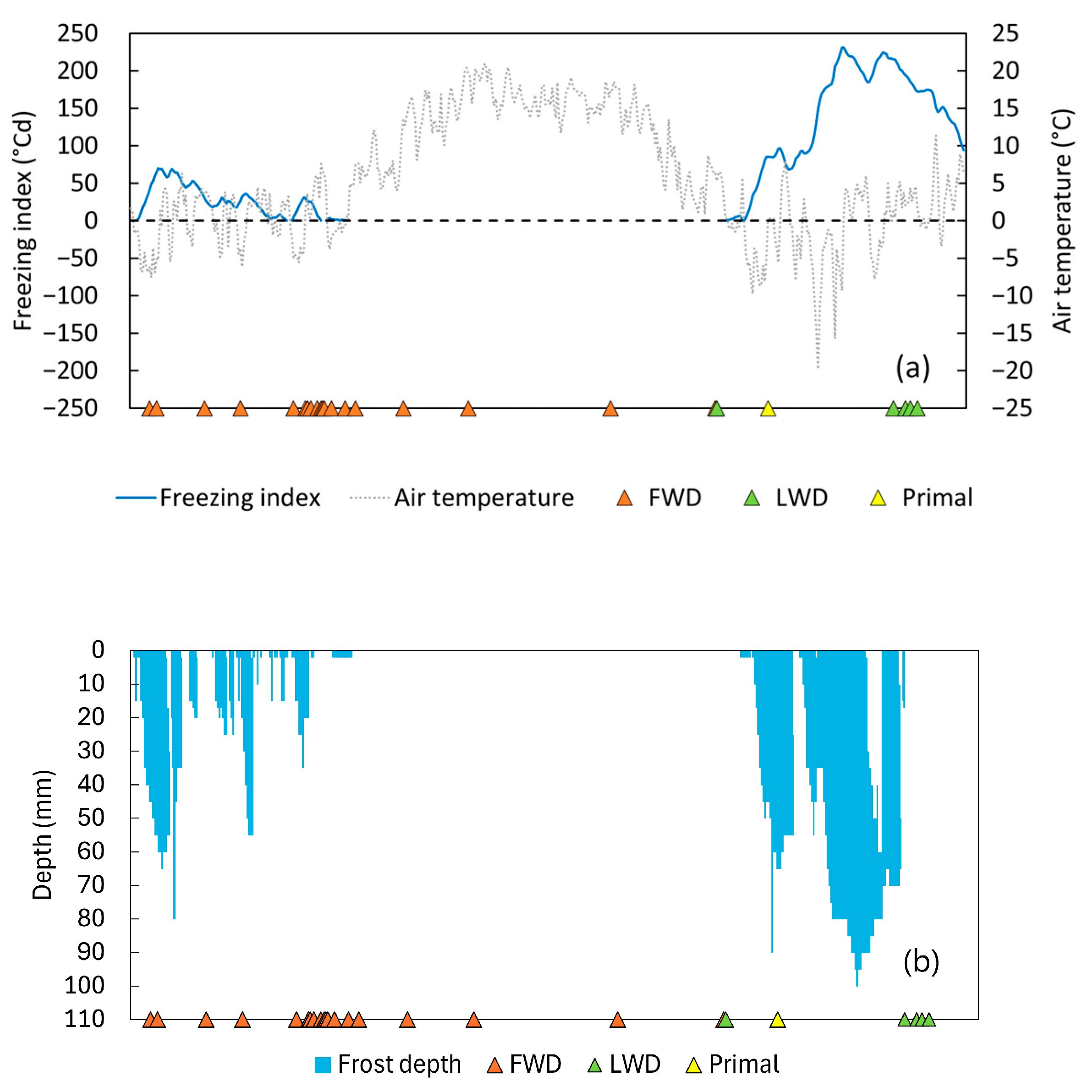
2.5. Climatic Conditions

As it was not possible to equip the cycle paths with temperature and moisture gauges, external temperature and precipitation data from the nearest weather station of the Swedish Meteorological and Hydrological Institute (SMHI), Malmslätt, were retrieved and analyzed. Frost depth data collected by the TRV from the nearest station, Ullevileden, in a road some six kilometres away from the cycle paths, was also used. The locations of these data collection points are shown in Figure 2. The data, which are presented in Figure 7, are used for the calculation of the freezing index [41], the assumption of frozen or partially frozen conditions of the cycle path structures, and the assumed effect of precipitation on the moisture content of the structures. The orange, green, and yellow triangles in the Figure indicate measurement dates. The solid blue line, corresponding to the left vertical axis in Figure 7a, indicates the freezing index. The dotted grey line, corresponding to the right vertical axis, indicates air temperature.

3. Results

The established DBPs SCI, BDI, and BCI, along with the proposed DBPs SCI_cp, BDI_cp, and BCI_cp have been calculated, according to Equations (1)–(3) and (6)–(8), respectively, and compared. To corroborate the suitability of the proposed DBPs, E_r and E₀ have been calculated, according to Equations (4) and (5), for all geophones where each of these parameters is applicable. This is followed by the results from the LWD measurements, and finally the transverse profile measurements and the calculation of the GEOM are presented. Metadata regarding the measurements and complete results of all calculations are presented in the open access public repository, found under the Data Availability Statement.

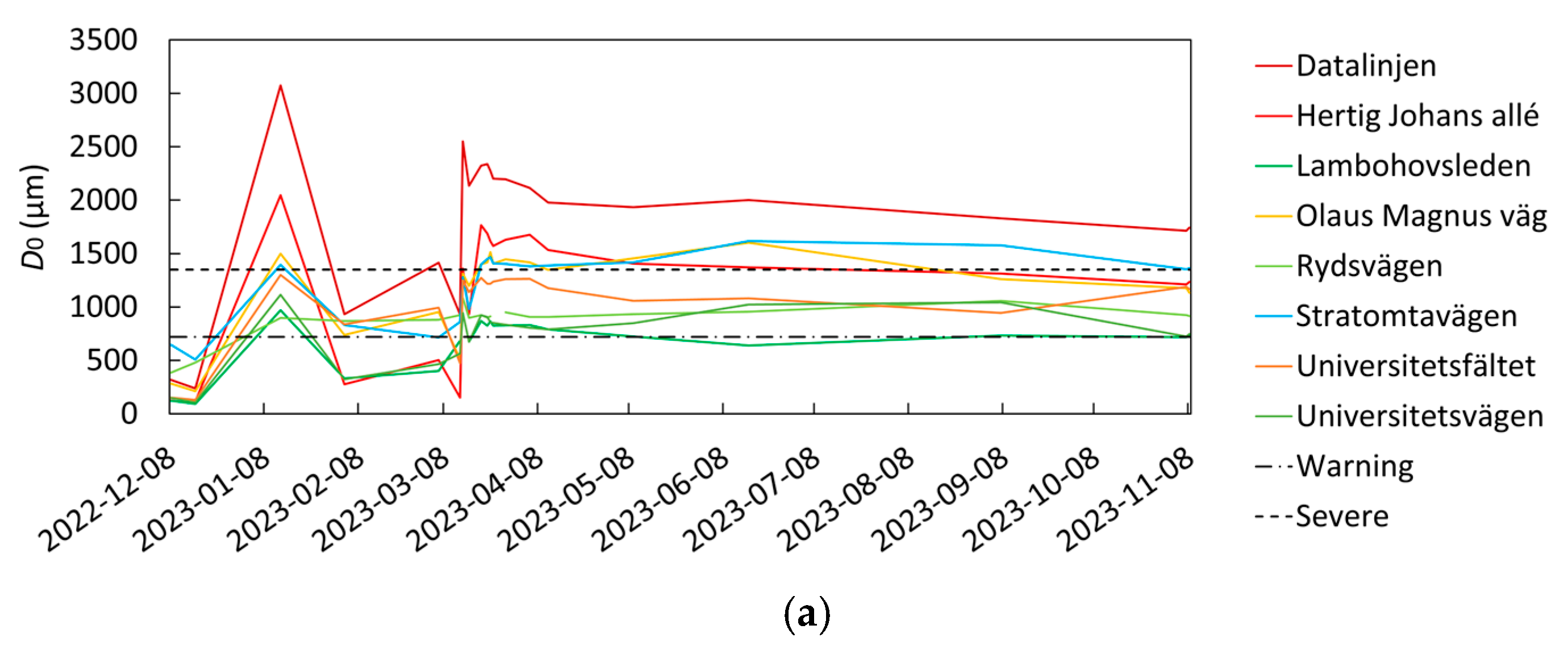
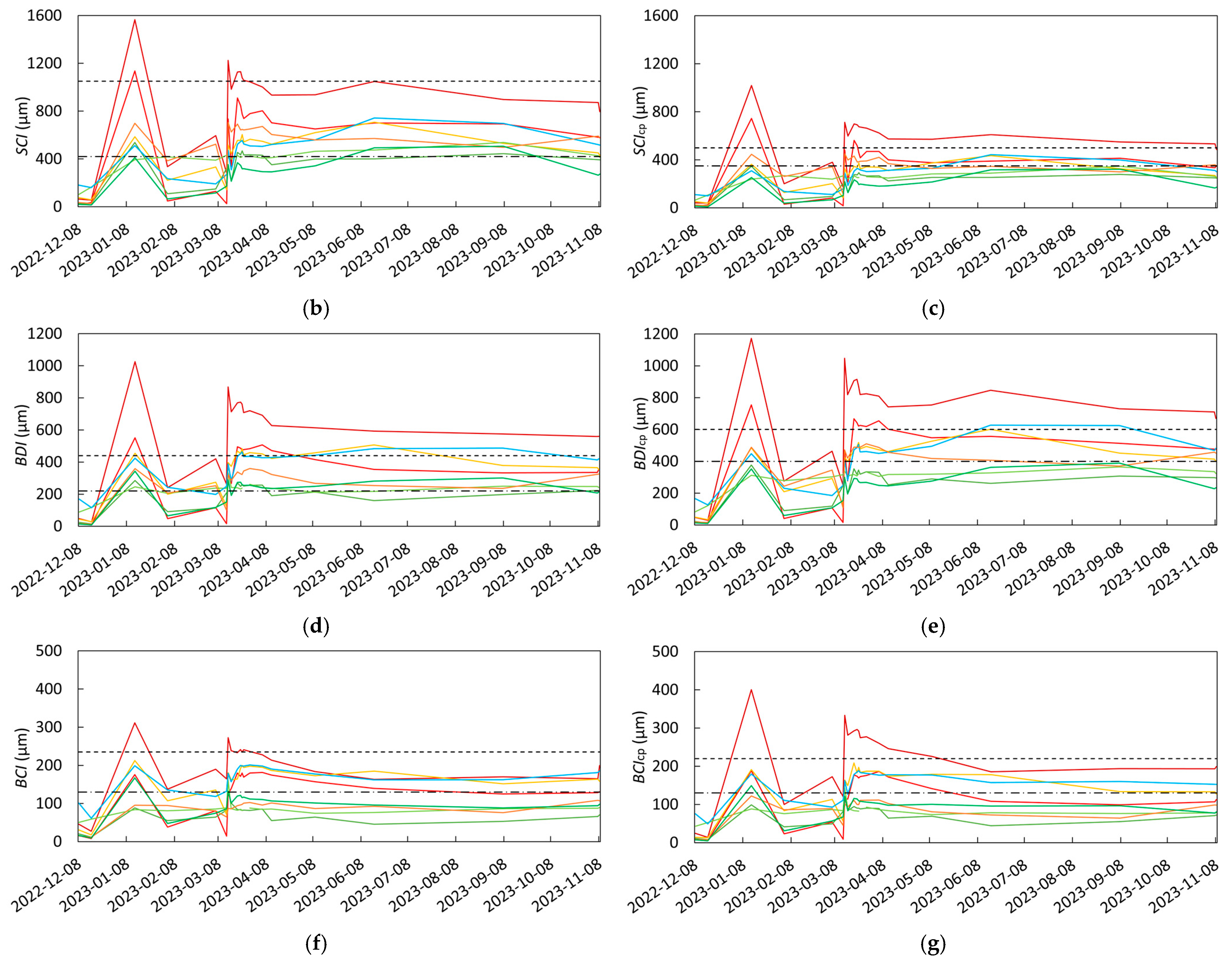
3.1. FWD Measurements

Figure 8 shows the D₀, SCI, BCI, BDI, SCI_cp, BDI_cp, and BCI_cp values, measured with the FWD in point 5 in Figure 4a for each cycle path, except for Olaus Magnus väg and Rydsvägen where point 6 has been used instead, and plotted as a function of time. As expected, the values are low for frozen conditions, i.e., the first two measurements conducted in December 2022. In general, the third measuring occasion, i.e., in January 2023, shows the highest values. From the middle of March and throughout the rest of the measuring cycle, air temperatures have been above zero, which from the middle of April results in quite even D₀ values. Except for Universitetsfältet, from September onwards the values decrease gradually.

Limit values for the proposed DBPs are tentatively suggested in

Table 3. Estimated limit values for the proposed DBPs.

Structural Condition Rating	Deflection Bowl Parameters (Based on FWD Data and Visual Inspection)
	SCIcp (µm)	BDIcp (µm)	BCIcp (µm)
Sound	<350	<400	<130
Warning	350–500	400–600	130–220
Severe	>500	>600	>220

, based on the results of the calculations of E₀ and E_r, and the conclusions from the visual inspection of the cycle paths included in this study. The cycle paths with the highest D₀ and DBP values—established as well as proposed—are the same ones that to some extent display visual distress, i.e., Datalinjen and Hertig Johans allé. Vice versa, the cycle paths with the minimum values of D₀ and DBPs, i.e., Lambohovsleden, Rydsvägen, and Universitetsvägen are also the ones that show the least distress at a visual inspection.

To control for the above-mentioned confounding effect of the small distance between the D₂₀₀ geophone and the edge of the loading plate, a comparison between the proposed DBP SCI_cp and the established DBP SCI has been conducted (Figure 9a). Corresponding comparisons have also been conducted for the BDI_cp versus BDI (Figure 9b), and the BCI_cp versus BCI (Figure 9c). There is a very strong correlation between the SCI_cp and SCI (R² > 0.99) and the BDI_cp and BDI (R² = 0.95), as well as between the BCI_cp and BCI (R² = 0.93). The BDI overlaps with both the BDI_cp and BCI_cp (see Figure 5), so this correlation might not be surprising. However, the BCI does not overlap with any of the proposed DBPs for cycle paths, but rather measures the condition of the SG, just like the BCI_cp. The difference is that the BCI_cp only covers the upper 150 mm of the SG, as opposed to the BCI which corresponds to a deeper subsection of the SG. A (strong) correlation could thus be expected. Still, there are important differences between the established and the proposed DBPs, which are further developed in the Section 4.

The D₀ from the FWD measurements varies with the lateral position, as shown in Figure 10, where purple thick lines indicate the minimum measured D₀, pink thick lines indicate the highest measured D₀, vertical black lines represent the position of the cycle path edge, and temperatures within brackets are pavement surface temperature as measured by the FWD. For frozen conditions, the D₀ is lower along the centre line of the cycle path than it is closer to the edges; however, for the critical situation, i.e., when D₀ is at its maximum, this relation is inverse, with a higher D₀ along the centre line. When the critical situation consists of freezing and subsequent thawing, this might be because the water content in the unbound layers is higher closer to the edges; therefore, it takes longer for the edge to freeze, and when frozen it takes longer to thaw. For Olaus Magnus väg, Figure 10b, however, where maximum D₀ occurs for hot pavement temperature (16th of June), this explanation is not valid. Still, the same phenomenon occurs.

Hence, the FWD measurements do not show “edge effect”, i.e., larger deflections close to the edges, as would be expected, but they do show that the stiffness of the structure varies between different lateral positions, especially for critical conditions, be it spring thaw or high summer temperatures.

The E_r has been calculated for all geophone positions for each of the FWD measurements (Equation (4)). According to the described principle of the E_r, the distance, r, to the geophone with the minimum E_r should represent the corresponding depth of r below the surface, where the structure is at its weakest.

Table 4. Calculated values and position of the minimum E_r, affected structural layer, and the DBP which best covers the affected subsection of the structure.

Normal Conditions (7–11 °C)
Cycle Path	Minimum Er (MPa)	Position with Minimum Er	Affected Structural Layer	Best Fit DBP
Datalinjen	49	D300	SB	BDIcp
Hertig Johans allé	71	D300	SB	BDIcp
Lambohovsleden	138	D300	SB	BDIcp
Olaus Magnus väg	62	D600	SG	BCIcp
Rydsvägen	86	D600	SG	BCI
Stratomtavägen	52	D600	SG	BCIcp
Universitetsfältet	78	D300	SB	BDIcp
Universitetsvägen	86	D600	SG	BCIcp
Spring Thaw Conditions
Cycle Path	Minimum Er (MPa)	Position with Minimum Er	Affected Structural Layer	Best Fit DBP
Datalinjen	31	D300	SB	BDIcp
Hertig Johans allé	51	D300	SB	BDIcp
Lambohovsleden	101	D300	SB	BDIcp
Olaus Magnus väg	48	D450	SG	BCIcp
Rydsvägen	64	D450	SB	BCIcp
Stratomtavägen	49	D450	SG	BCIcp
Universitetsfältet	77	D300	SB	BDIcp
Universitetsvägen	61	D450	SB	BCIcp
Hot Pavement Temperature (>25°C)
Cycle Path	Minimum Er (MPa)	Position with Minimum Er	Affected Structural Layer	Best Fit DBP
Datalinjen	49	D300	SB	BDIcp
Hertig Johans allé	69	D300	SB	BDIcp
Lambohovsleden	154	D200	SB	SCI
Olaus Magnus väg	52	D300	SB	BDIcp
Rydsvägen	75	D900	SG	BCI
Stratomtavägen	53	D300	SG	BDIcp
Universitetsfältet	87	D600	SG	BCI
Universitetsvägen	86	D300	SB	BDIcp

presents the geophone position of the minimum E_r, to which structural layer this E_r corresponds, and which DBP in this study best covers this subsection of the structure. The results have been categorized into the scenarios “normal conditions”, i.e., autumn conditions (7–11 °C), “spring thaw conditions” (where it is evident from data that large deflections occur right after a period of frozen conditions), and “hot pavement temperatures” (>25 °C). Frozen conditions have been excluded as they do not pose any problem for the structural stability. As seen from Table 4, it is in the SB or the upper parts of the SG that the minimum E_r are found, except for Rydsvägen, where it seems to be located further down in the SG. The results indicate that in general, the proposed DBPs are adequate in covering the structural weaknesses in cycle path structures.

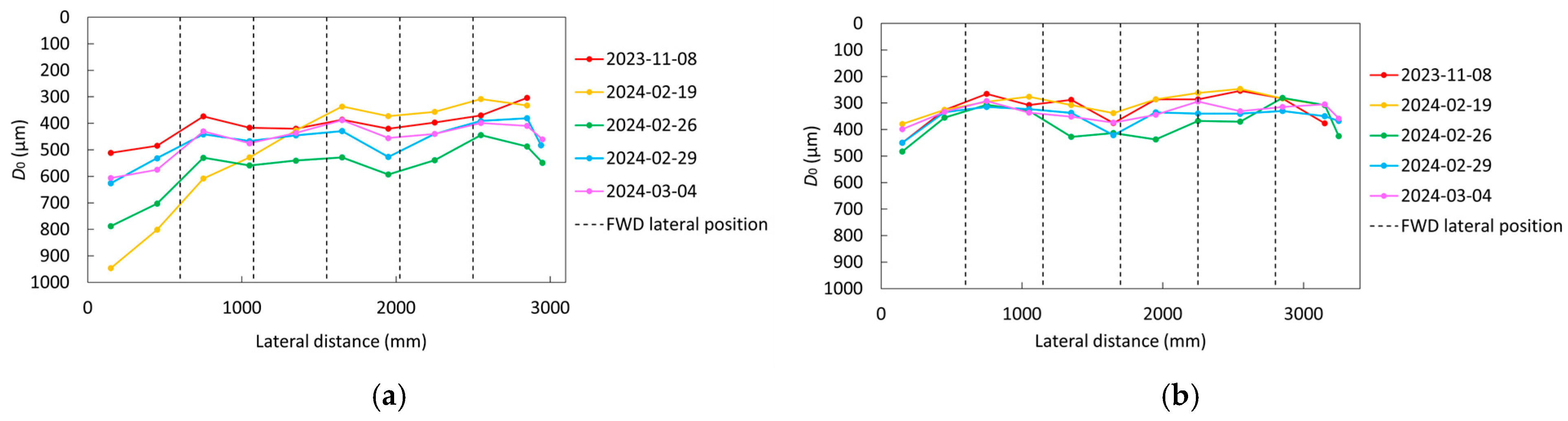
3.2. LWD Measurements

For the LWD measurements, which were possible to conduct closer to the edges, the suspected edge effect was shown for all the cycle paths, though not for all the measuring occasions (Figure 11). In Figure 11, dashed vertical lines indicate the lateral positions of the FWD measurements and the vertical axis represents the cycle path edges; hence, the horizontal scale differs between subfigures. The left side of Datalinjen (Figure 11a) presents large deflections, especially for the measurements on the 19th of February 2024. When compared with the frost depth data from Ullevileden (Figure 3b), it seems plausible that this is due to thawing in the UGLs, which results in a high moisture content. As there is a crack about 750 mm from the left edge and the cross fall is from right to left (see Figure 12), it is also possible that melted snow on the surface seeps into the UGLs through this crack, leaving the left edge considerably weakened. The large deflections on the right edge of Universitetsvägen (Figure 11h) from the 26th of February 2024 onwards are believed to be due to a thin longitudinal crack about 150 mm from the edge that widened during the measuring period.

Some of the cycle paths, e.g., Figure 11b,e, displayed larger deflections in the centre than in the lateral positions between the centre and the edge, as indicated by the FWD measurements in Figure 10.

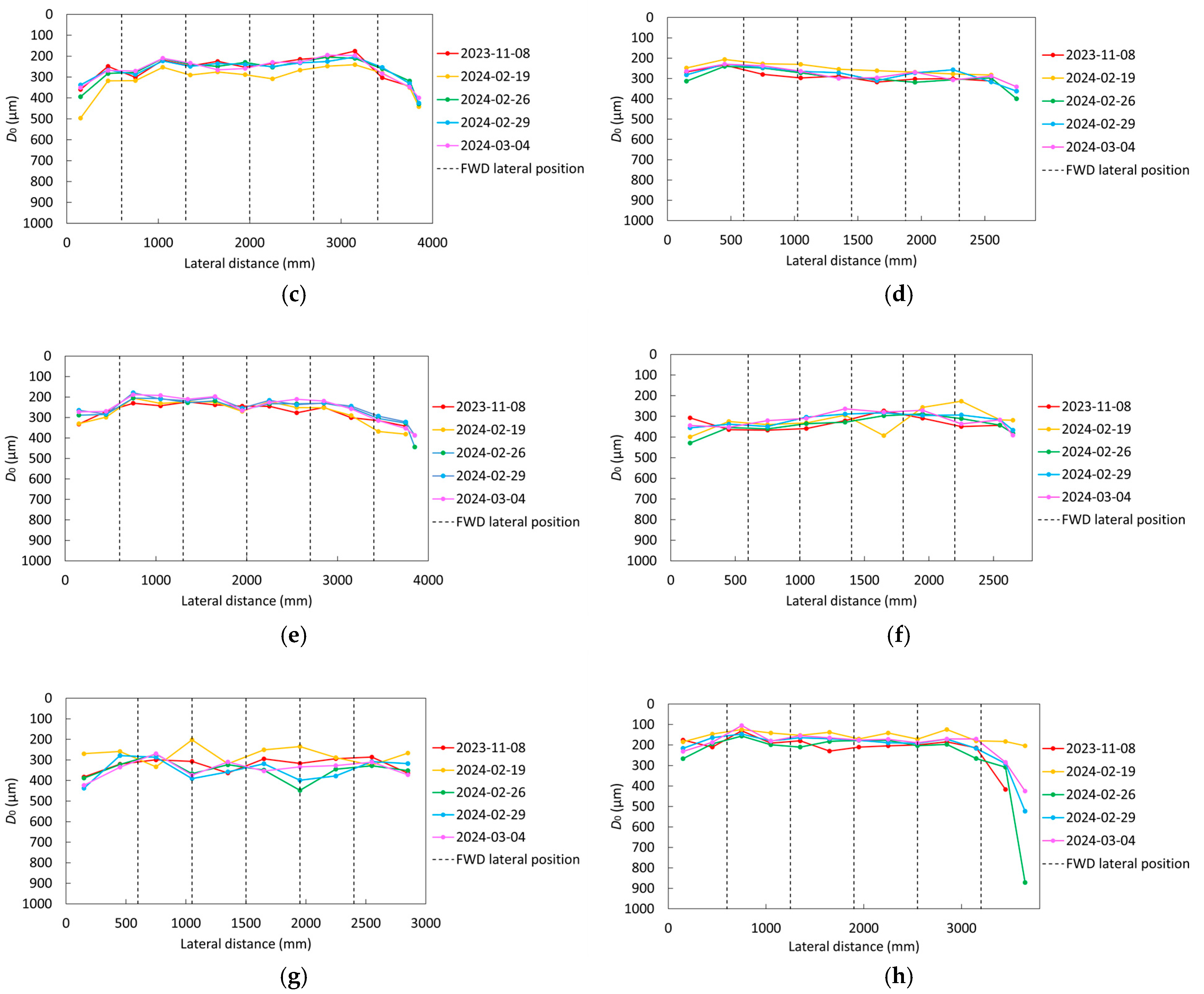
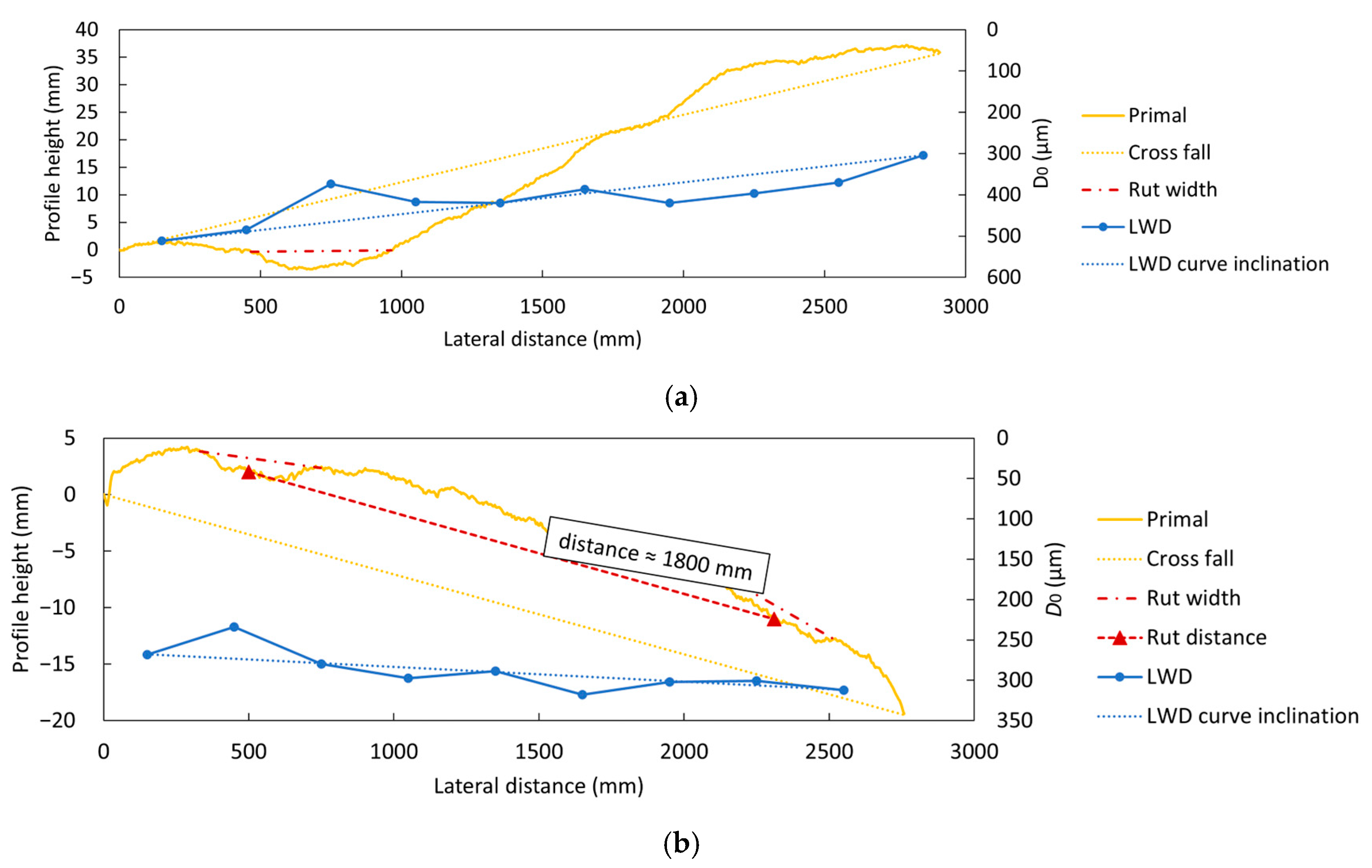
3.3. Transverse Profile Measurements

In general, the transverse profiles of the cycle paths show little signs of ruts, except for Datalinjen (Figure 12a), where a rut on the left-hand side is clearly observable through visual inspection, and to some extent on Olaus Magnus väg (Figure 12b). In the latter case, it is not directly observable by the naked eye in dry conditions, but it was detected by the transverse profile measurements. The cross fall of the cycle paths has been added manually, through interpolation, to the transverse profiles that were measured by the Primal equipment. Primal measurements and cross fall correspond to the left y-axis in the figure while the D₀, for the LWD measurements and the LWD inclination curve, correspond to the right y-axis. What is notable is that the peaks in the LWD curve, i.e., lower deflections, coincide quite well with the lateral position of the ruts. The fact that the ruts are wide and shallow indicates that it is in the lower parts of the UGLs that plastic deformation has occurred [2]. In the case of Datalinjen, there is no clear tendency to larger measured deflections on the right edge, and for Olaus Magnus väg, the “edge effect” is modest. The inclination of the D₀ curve of the LWD (blue dotted line) in Figure 12 also seems to coincide with the direction of the cross fall (yellow dotted line), giving larger D₀ toward the lower end of the cycle path surface. This correlation is confirmed for all the cycle paths except for Universitetsfältet. However, as Table 1 shows, the measured cross fall at Universitetsfältet is the lowest (0.4%) of all the cycle paths.

Geometries from the construction plans have been used to calculate the GEOM for the different cycle paths. The results show that the effect is clearest for the right edge on Rydsvägen, where a side slope of 1:3, in combination with the lack of a shoulder, gives a GEOM of 6 at a distance of 0.15 m from the edge. If a shoulder of 0.15 m, which is the narrowest shoulder being used for any of the other cycle paths in the study, were to be added, the GEOM would drop to 2.8 for the same measuring position, theoretically lowering the degradation rate from rutting by more than 100 percent.

4. Discussion

4.1. Methods and Data

Realistic E values, as stated in [14], assume 10 °C for the AC layer and an optimum moisture content for the UGLs. It is assumed that the temperature only has a limited effect on such thin asphalt layers, which is supported in previous studies [31], but in practice it is hard to know the moisture content without actually measuring it. An ideal setup for this type of study would be to conduct measurements on structures instrumented with frost rods and moisture gauges. However, for already existing cycle paths, this would imply an intervention which would alter their properties. Therefore, external data for frost depth and precipitation have been collected and assumptions have been made regarding the effect of these parameters on the structures. It would be beneficial to complement this study with similar investigations on instrumented cycle paths in the future to determine the direct relation between the temperature and moisture content with the structural stability of the inherent structural layers. What can be deduced from the results of this study, however, and is consistent with previous research, is that drainage is of utmost importance [7], as a small change in moisture content can have a high impact on the load-bearing capacity of the unbound materials. The three cycle paths that performed best with regard to the proposed BDPs, i.e., Lambohovsleden, Rydsvägen, and Universitetsvägen, are the ones equipped with drainage pipes.

4.2. Results

Back-calculated E values for the different structures confirmed that they showed poor fit with stated realistic values, in general, and have thus not been further analyzed.

The proposed metrics, SCI_cp, BDI_cp, and BCI_cp, with the three levels—sound, warning, and severe—work as an easy practical way to categorize the structural stability of cycle paths. They permit the identification of weaknesses in the cycle path structures and the structural layer that is most affected. The proposed DBPs are based on previously existing DBPs [34] and adjusted to better suit cycle paths. There is a very strong correlation (R² = 0.99) between the proposed DBP SCI_cp and the established DBP SCI. However, the SCI_cp is theoretically more adapted to represent the part of the total deflection that stems from the AC and BC for normal layer thicknesses on cycle paths (30–60 mm and 80–120 mm, respectively), which is why its use is recommended. There is also a strong correlation between the proposed BDI_cp and the established BDI (R² = 0.95), and between the proposed BCI_cp and the established BCI (R² = 0.92). Still, there are some important differences which indicate that the load-bearing capacity varies within the same structural layer. Through the calculations of E₀ and E_r, it was found that the weakest structural sections were generally located at a depth of 300–450 mm below the surface, which corresponds to the subbase and the upper 150 mm of the SG. This is consistent with previous research that indicates that for the TSAPs, the maximum plastic deformations from the wheel loads are likely to occur somewhere between 150 and 550 mm below the surface [37,42]. In analogy with SCI_cp compared to SCI, BDI_cp and BCI_cp are theoretically more adapted than BDI and BCI to the structural design of cycle paths, often having total thicknesses of only 300 mm (see Table 1).

An example of this is that, even though this very strong correlation between SCI and SCI_cp exists at Datalinjen, SCI (D₀−D₃₀₀) shows a clear peak for the measurement conducted on the 16th of June (Figure 8b), whereas the SCI_cp (D₀−D₂₀₀) does not show this peak as clearly (Figure 8c). The peak is however clearly visible for the BDI_cp (D₂₀₀−D₄₅₀) (Figure 8e), but not for the BDI (D₃₀₀−D₆₀₀) (Figure 8d). From this, it can be deduced that the peak deflection is situated between D₂₀₀ and D₃₀₀. Due to the thin AC (30 mm) and BC (120 mm) of the cycle path, along with the described principle for the E_r, this places the cause of the deflection peak at a depth of 200–300 mm below the surface, i.e., in the SB. This is also confirmed by the calculations of the E_r in Table 4, where the minimum E_r is detected close to the D₃₀₀ geophone. However, the trend of the D₀ curve in Figure 8a indicates a decrease from the beginning of April to November, which is consistent with a decreasing moisture content in the UGLs after the spring thaw period [41]. Since the 17th of May there was no precipitation (Figure 7c), which makes it very likely that this peak in the SCI curve is the result of the hot pavement temperature (41 °C) rather than a sudden increase in moisture content of the UGLs. The high temperature should affect the AC layer, which only constitutes the upper 30 mm of the structure in this case, rather than the UGLs. The condition of the upper 30 mm of this structure should however be detected by both the SCI and SCI_cp. A plausible explanation for this phenomenon is that the loss of stiffness of the AC layer due to the high pavement temperature is not distributed as larger deflections in the thin AC or BC, but instead the load is transferred deeper down in the structure, where it can be perceived as larger deflections in the SB.

A comparison between the BCI (D₆₀₀−D₉₀₀) (Figure 8e) and the BCI_cp (D₄₅₀−D₆₀₀) (Figure 8f), despite the strong correlation, indicates a more distinct difference between Datalinjen and the rest of the investigated cycle paths for the BCI_cp than for the BCI. This is consistent with the fact that Datalinjen is the only one of the cycle paths that displays generalized distress, in the form of a rut with a classic longitudinal bottom-up fatigue crack in the middle, along the left side of the cycle path (Figure 2a). From Figure 8g and Figure 11, the D₀ for suspected thawing situations (13 October 2023 for FWD and 19 February 2024 for LWD) is considerably higher than for the rest of the cycle paths. Therefore, it is probable that the unsealed crack contributes to water infiltration into the UGLs. A low permeability of the SG, and a lack of proper drainage, is also likely to give rise to high levels of moisture in the upper 100–500 mm of the SG [7]. However, as Table 1 indicates, there are only minor differences between the structural properties of Datalinjen and Olaus Magnus väg, which makes it likely that the consistent differences in D₀ between these two cycle paths are related to the increased water infiltration through the crack at Datalinjen.

These are indications that the proposed DBPs—SCI_cp, BDI_cp, and BCI_cp—better reflect the effects of the (simulated) traffic loads on cycle paths than the (for roadways) established DBPs, i.e., SCI, BDI, and BCI. By applying the established DBPs rather than the proposed DBPs, maintenance actions risk focusing on the wrong parts of the structure. The consequences could possibly lead to a sub-optimization of resources by implementing costly measures without actually attending to the cause of the problem, which then may recur sooner than expected. The suggested limit values for the proposed DBPs work well for the cycle paths investigated in this study, but they need to be validated and confirmed or adjusted by further studies.

A possible explanation for the “m-shaped” curves in Figure 11b,c is differences in the degree of compaction between the different lateral positions. Due to the width of these cycle paths (≈3 m), in combination with the track width of the heavy maintenance vehicles (1.85–2 m) [2], the centre of the cycle path will never be directly under the wheel load from such a vehicle. It is plausible to assume that when a maintenance vehicle transits the cycle path, they will try to maintain a lateral position as centred as possible, which statistically would place the centre of the wheel loads 0.5–0.6 m from the edge, thus compacting these lateral positions more than in the middle or closer to the edges. For the three widest cycle paths in the study where more heterogeneity in the lateral positions of the vehicles is expected, Lambohovsleden, Rydsvägen, and Universitetsvägen (≈4 m), the shape of the curve is more uniform in the different lateral positions except for the edges that are tilted down. The lateral distance between the ruts on Olaus Magnus väg supports this theory. The fact that these ruts are shallow and wide indicates that it is in the lower parts of the structure that these plastic deformations have occurred. This complies with the minimum calculated E_r, which indicates that it is located in the SG for this cycle path.

D₀ measurements with an LWD are sufficient to capture the effect of larger deflections closer to the cycle path edges, where they will actually be exposed to the heavy loads from traffic (Figure 13).

There is no support in the collected data to suggest that the difference in the number of passings of maintenance vehicles between the cycle paths that are sweep-salted (N ≈ 200/year) and the gritted ones (N ≈ 20/year) should have any effect on the degradation. The three cycle paths classified as sound from the proposed metric are all sweep-salted in wintertime.

5. Conclusions

The proposed DBPs seem to be able to pinpoint the weak sections or conditions and give indications of whereabouts in the structure the weaknesses are situated in, thus facilitating suitable maintenance actions. More studies are however needed to validate the proposed limit values.

From the results in this study, some general conclusions regarding the structural design of cycle paths can be drawn. The most important aspect seems to be assuring the sufficient drainage of the structure. Moreover, wider cycle paths (≥3.8 m) seem to have less problems with structural instability, and a shoulder, even as narrow as 0.15 m, can reduce the degradation rate of the cycle path close to the edge significantly, while improving the drainage at the same time.

The load-bearing capacity varies across the cycle path. The edges and centre line are weaker than positions in between. The edges are more of a concern than the centre line, as the centre line is less likely to be loaded at all. The load-bearing capacity also varies considerably with the seasons of the year, with low points during thawing periods and in some cases on the hottest summer days. A recommendation is thus to avoid transiting the cycle paths with heavy vehicles during these situations. The use of LWD for the structural evaluations of cycle paths is a promising approach. However, further studies are needed to establish the maximum depth at which the LWD load impulses affect the structure.

In conclusion, these are the highlights of this study:

• The traditional approach of load-bearing capacity evaluations with FWD measurements along the centre line is generally not a viable option for cycle paths.
• LWD measurements are easier to conduct than FWD measurements close to the cycle path edges and are thus a promising tool for the evaluation of load-bearing capacity close to the pavement edge on cycle paths. More studies are however needed to determine the accuracy and repeatability of the LWD measurements.
• Compaction from traffic loads provides better structural stability in the lateral positions between the centre line and the edges.
• Wider cycle paths (>3.8 m), designed with shoulders and sufficient drainage solutions, are important factors for increasing the structural stability of the cycle paths.
• The proposed Deflection Bowl Parameters SCI_cp, BDI_cp and BCI_cp are useful tools to detect weaknesses in different structural parts of the investigated cycle paths.

References

1. Larsson, M.; Niska, A.; Erlingsson, S. Degradation of Cycle Paths—A Survey in Swedish Municipalities. CivilEng 2022, 3, 184–210. [Google Scholar] [CrossRef]
2. Ekdahl, P. Bära Eller Brista. Handbok I Tillståndsbedömning Av Belagda Gator Och Vägar; Swedish Association of Local Authorities and Regions: Stockholm, Sweden, 2019. (In Swedish) [Google Scholar]
3. Nyberg, P.; Björnstig, U.; Bygren, L.-O. Road characteristics and bicycle accidents. Scand. J. Soc. Med. 1996, 24, 293–301. [Google Scholar] [CrossRef] [PubMed]
4. Schepers, P.; Theuwissen, E.; Velasco, P.N.; Niaki, M.N.; van Boggelen, O.; Daamen, W.; Hagenzieker, M. The relationship between cycle track width and the lateral position of cyclists, and implications for the required cycle track width. J. Saf. Res. 2023, 87, 38–53. [Google Scholar] [CrossRef] [PubMed]
5. Botma, H. Method to Determine Level of Service for Bicycle Paths and Pedestrian-Bicycle Paths. Transp. Res. Rec. 1995, 1502, 38–44. [Google Scholar]
6. Wierbos, M.J.; Knoop, V.L.; Hänseler, F.S.; Hogendoorn, S.P. Capacity, Capacity Drop, and Relation of Capacity to the Path Width in Bicycle Traffic. Transp. Res. Rec. 2019, 2673, 693–702. [Google Scholar] [CrossRef]
7. Thom, N. Principles of Pavement Engineering, 2nd ed.; Emerald Publishing Limited: London, UK, 2014. [Google Scholar]
8. Charlier, R.; Hornych, P.; Srsen, M.; Hermansson, Å.; Bjarnason, G.; Erlingsson, S.; Pavsic, P. Water Influence on Bearing Capacity and Pavement Performance: Field Observations. In Water in Road Structures. Movement, Drainage and Effects, 1st ed.; Dawson, A., Ed.; Springer: Dordrecht, The Netherlands, 2009; Volume 5, pp. 175–192. [Google Scholar] [CrossRef]
9. Aksnes, J. A Study of Load Responses Towards the Pavement Edge. Ph.D. Thesis, Norwegian University of Science and Technology, Trondheim, Norway, August 2002. [Google Scholar]
10. Dablanc, L.; Beziat, A. Parking for Freight Vehicles in Dense Urban Centers—The Issue of Delivery Areas in Paris; MetroFreight Center of Excellence: Marne la Vallee, France, 2015. [Google Scholar]
11. Korkiala-Tanttu, L. Calculation Method for Permanent Deformation of Unbound Pavement Materials. Ph.D. Thesis, Helsinki University of Technology, Helsinki, Finland, 30 January 2009. [Google Scholar]
12. Bianchini, A. Thin asphalt pavement performance equation through direct computation of falling weight deflectometer-derived strains. Int. J. Pavement Eng. 2014, 15, 831–839. [Google Scholar] [CrossRef]
13. Van Gurp, C. Use of Falling Weight Deflectometers in Pavement Evaluation. In Final Report of the Action; COST: Brussels, Belgium, 2005. [Google Scholar]
14. Salour, F. Utvärdering Av Vägkonstruktioners Bärighet Med Fallviktsapparat; Swedish Road Administration: Borlänge, Sweden, 2020. (In Swedish) [Google Scholar]
15. Martínez Arguelles, G.; Fuentes, L.G.; Torregroza Aldana, L.M. Review of the pavement management system of the Bogotá bike-path network. Rev. Ing. Construcción 2011, 26, 150–170. [Google Scholar] [CrossRef]
16. Vavrova, M.; Chang, C.M. Incorporating Livability into Transportation Asset Management Practices through Bikeway Quality Networks. Transp. Res. Rec. 2019, 2673, 407–414. [Google Scholar] [CrossRef]
17. Fladvad, M.; Karlsson, H. Dimensjonering Av Gang-Og Sykkelvegløsninger. Vurdering Av Krav I N200 Vegbygging; SINTEF: Trondheim, Norway, 2022. (In Norwegian) [Google Scholar]
18. Ordaz, M.; Doyle, J.D.; Howard, I.L. Light Weight Deflectometer Evaluation of Low-Volume Road Structural Deterioration under Rapidly Increased Traffic Patterns. Transp. Res. Rec. 2024, 2678, 948–966. [Google Scholar] [CrossRef]
19. Kestler, M.A.; Humphrey, D.N.; Steinert, B.C. Portable Falling-Weight Deflectometers for Tracking Seasonal Stiffness Variations in Asphalt-Surfaced Roads. In Proceedings of the Transportation Research Board 85th Annual Meeting, Washington, DC, USA, 22–26 January 2006. [Google Scholar]
20. Horak, E.; Maina, J.; Guiamba, D.; Hartman, A. Correlation Study with the Light Weight Deflectometer in South Africa. In Proceedings of the 27th Southern African Transport Conference, Pretoria, South Africa, 7–11 July 2008. [Google Scholar]
21. Sawangsuriya, A. Correlation between LWD and FWD deflections for asphalt pavement. In Proceedings of the 11th International Conference on the Bearing Capacity of Roads, Railways and Airfields, Trondheim, Norway, 28–30 June 2022. [Google Scholar]
22. FEHRL. VTI Primal Longitudinal Profile Instrument. Available online: https://www.fehrl.org/facilities/detail/111 (accessed on 25 September 2024).
23. TRV. Krav—VGU, Vägars Och Gators Utformning (Requirements—VGU, Design of Roads and Streets); Swedish Transport Administration: Borlänge, Sweden, 2022. (In Swedish) [Google Scholar]
24. Karakas, A.S. Aging Effects on Mechanical Characteristics of Multi-Layer Asphalt Structure. In Modified Asphalt, 1st ed.; Rivera Armenta, J.L., Salazar-Cruz, B.A., Eds.; IntechOpen: London, UK, 2018. [Google Scholar]
25. Blab, R.; Litzka, J. Measurements of the Lateral Distribution of Heavy Vehicles and Its Effect on the Design of Road Pavements. In Proceedings of the 4th International Symposium on Heavy Vehicle Weights and Dimensions, Ann Arbor, MI, USA, 25–29 June 1995. [Google Scholar]
26. Arraigada, M.; Partl, M. Pavement Distress from Channelized and Lateral Wandering Loads Using Accelerated Pavement Tests. In Proceedings of the 9th International Conference on Maintenance and Rehabilitation of Pavements—Mairepav9, Dübendorf, Switzerland, 1–3 June 2020. [Google Scholar]
27. Sinamnis, R.; Woods, L. Traffic channelisation and pavement deterioration: An investigation of the role of lateral wander on asphalt pavement rutting. Int. J. Pavement Eng. 2023, 24, 2118272. [Google Scholar] [CrossRef]
28. Mallick, R.B.; El-Korchi, T. Pavement Engineering. Principles and Practice, 2nd ed.; CRC Press: Boca Ratón, FL, USA, 2013. [Google Scholar]
29. Niska, A.; Blomqvist, G. Sweep-salting—A method for winter maintenance of bicycle paths. In Proceedings of the 15th International Winter Road Congress, Gdansk, Poland, 20–23 February 2018. [Google Scholar]
30. Karlsson, H.; Rise, T. Effekt Av Salt Og Teleskader På Gang-Og Sykkelveger, En Litteraturstudie; Sintef: Trondheim, Norway, 2019. (In Norwegian) [Google Scholar]
31. Howard, I.L. Preservation of Low-Volume Flexible Pavement Structural Capacity by Use of Seal Treatments. Transp. Res. Rec. 2011, 2204, 45–53. [Google Scholar] [CrossRef]
32. Martin, T.; Choummanivong, L.; Toole, T. New pavement deterioration models for sealed low volume roads in Australia. In Proceedings of the 8th International Conference on Managing Pavement Assets, Santiago, Chile, 15–19 November 2019. [Google Scholar]
33. TRV. Överbyggnad Väg, Dimensionering Och Utformning (Design of Road Super Structures); Swedish Transport Administration: Borlänge, Sweden, 2023. (In Swedish) [Google Scholar]
34. Horak, E.; Emery, S. Falling Weight Deflectometer Bowl Parameters as Analysis Tool for Pavement Structural Evaluations. In Proceedings of the 22nd ARRB Conference: Research into Practice, Canberra, Australia, 29 October–2 November 2006. [Google Scholar]
35. Cekerevac, C.; Baltzer, S.; Charlier, R.; Chazallon, C.; Erlingsson, S.; Gajewska, B.; Hornych, P.; Kraszewski, C.; Pavisc, P. Water Influence on Mechanical Behaviour of Pavements: Experimental Investigation. In Water in Road Structures. Movement, Drainage and Effects, 1st ed.; Dawson, A., Ed.; Springer: Dordrecht, The Netherlands, 2009; Volume 5, pp. 217–242. [Google Scholar] [CrossRef]
36. Horak, E.; Maree, J.; van Wijk, A. Procedures for Using Impulse Deflectometer (IDM) Measurements in the Structural Evaluation of Pavements. In Annual Transportation Convention; South African Council for Scientific and Industrial Research, Division of Roads and Transport Technology: Pretoria, South Africa, 1989. [Google Scholar]
37. Korkiala-Tanttu, L.; Laaksonen, R. Permanent Deformations of Unbound Materials of Road Pavement in Accelerated Pavement tests. In Proceedings of the 13th European Conference on Soil Mechanics and Geotechnical Engineering, Prague, Czech Republic, 25–28 August 2003. [Google Scholar]
38. Maree, J.H.; Bellekens, R.J.L. The Effect of Asphalt Overlays on the Resilient Deflection Bowl Response of Typical Pavement Structures; Department of Transport, Chief Directorate National Roads: Pretoria, South Africa, 1991. [Google Scholar]
39. Department of Transport and Main Roads. Pavement Rehabilitation Manual; The State of Queensland: Brisbane, Australia, 2020. [Google Scholar]
40. Korkiala-Tanttu, L.; Dawson, A. Effects of side slope on low-volume road pavement performance: A full-scale assessment. Can. Geotech. J. 2008, 45, 853–866. [Google Scholar] [CrossRef]
41. Doré, G.; Zubeck, H.K. Cold Regions Pavement Engineering, 1st ed.; ASCE: Reston, VA, USA, 2009. [Google Scholar]
42. Leischner, S.; Wellner, F.; Canon Falla, G.; Oeser, M.; Wang, D. Design of Thin Surfaced Asphalt Pavements. In Proceedings of the 3rd International Conference on Transportation Geotechnics, Guimarães, Portugal, 4–7 September 2016. [Google Scholar]
Figure 1. (a) The location of the measured cycle paths, along with frost data and weather data collection points. (b) The soil types that constitute the SG for the cycle paths.
Infrastructures 10 00007 g001
Figure 2. The municipal cycle paths in the study: (a) Datalinjen, (b) Hertig Johans allé, (c) Lambohovsleden, (d) Olaus Magnus väg, (e) Rydsvägen, (f) Stratomtavägen, (g) Universitetsfältet, and (h) Universitetsvägen.
Infrastructures 10 00007 g002
Figure 3. Measurement equipment used in the study: (a) the FWD, (b) the LWD, and (c) the Primal longitudinal profile instrument.
Infrastructures 10 00007 g003
Figure 4. (a) The setup for the FWD measurements, and (b) the setup for the LWD measurements. The light grey rectangular area is the cycle path and the dark grey circles are the measuring points. Dashed line indicates the centre line of the cycle path.
Infrastructures 10 00007 g004aInfrastructures 10 00007 g004b
Figure 5. A comparison between structural parts of (a) a cycle path, and (b) a low-volume road, all of which are theoretically covered by SCI, BCI, and BDI, versus the proposed DBPs SCIcp, BDIcp, and BCIcp.
Infrastructures 10 00007 g005
Figure 7. (a) Air temperature and freezing index, (b) frost penetration depth at Ullevileden, and (c) precipitation at SMHI, Malmslätt, during the measurement cycle.
Infrastructures 10 00007 g007aInfrastructures 10 00007 g007b
Figure 8. Variations in (a) D0, (b) SCI, (c) SCIcp, (d) BDI, (e) BDIcp, (f) BCI, and (g) BCIcp in the middle of the cycle paths during the FWD measurement year cycle. Limit values (dotted and dash-dotted lines) according to Table 2 and Table 3.
Infrastructures 10 00007 g008aInfrastructures 10 00007 g008b
Figure 9. Correlation between (a) SCIcp and SCI, (b) BDIcp and BDI, and (c) BCIcp and BCI.
Infrastructures 10 00007 g009
Figure 10. Variation of D0 from FWD measurements for different lateral positions on (a) Datalinjen and (b) Olaus Magnus väg.
Infrastructures 10 00007 g010
Figure 11. LWD measurements for (a) Datalinjen, (b) Hertig Johans allé, (c) Lambohovsleden, (d) Olaus Magnus väg, (e) Rydsvägen, (f) Stratomtavägen, (g) Universitetsfältet, and (h) Universitetsvägen.
Infrastructures 10 00007 g011aInfrastructures 10 00007 g011b
Figure 12. The transverse profiles of (a) Datalinjen and (b) Olaus Magnus väg.
Infrastructures 10 00007 g012
Figure 13. Heavy vehicle, with track width almost as wide as the cycle path, transiting Universitetsfältet in March 2024.
Infrastructures 10 00007 g013