LSTM+MA: A Time-Series Model for Predicting Pavement IRI

Abstract

The accurate prediction of pavement performance is essential for transportation administration or management to appropriately allocate resources road maintenance and upkeep. The international roughness index (IRI) is one of the most commonly used pavement performance indicators to reflect the surface roughness. However, the existing research on IRI prediction mainly focuses on using linear regression or traditional machine learning, which cannot take into account the historical effects of IRI caused by climate, traffic, pavement construction and intermittent maintenance. In this work, a long short-term memory (LSTM)-based model, LSTM+MA, is proposed to predict the IRI of pavements using the time-series data extracted from the long-term pavement performance (LTPP) dataset. Effective preprocessing methods and hyperparameter fine-tuning are selected to improve the accuracy of the model. The performance of the LSTM+MA is compared with other state-of-the-art models, including logistic regressor (LR), support vector regressor (SVR), random forest (RF), K-nearest-neighbor regressor (KNR), fully connected neural network (FNN), XGBoost (XGB), recurrent neural network (RNN) and LSTM. The results show that selected preprocessing methods can help the model learn quickly from the data and reach high accuracy in small epochs. Also, it shows that the proposed LSTM+MA model significantly outperforms other models, with an R² of 0.965 and a mean square error (MSE) of 0.030 in the test datasets. Moreover, an overfitting score is proposed in this work to represent the severity degree of the overfitting problem, and it shows that the proposed model does not suffer severely from overfitting.

1. Introduction

Pavement roughness is defined as the deviation of a pavement surface from an actual surface, with characteristic dimensions that affect vehicle dynamics, ride quality, dynamic loads, and drainage [1]. It is considered one of the most significant indicators of pavement condition, as it dramatically affects driving comfort and safety, especially for high-speed-limit roads [2]. Various factors, including construction quality, maintenance, distress, climate, and traffic, all affect pavement roughness [3]. Macrotexture, surface material, and longitudinal and transverse slope also play crucial roles in determining pavement roughness. The interactions between these factors make the field of pavement roughness evaluation and prediction highly complex, requiring comprehensive analysis to accurately model and manage pavement condition [4]. International roughness index (IRI) is widely recognized as a key indicator of pavement functional condition and ride quality, which is extensively utilized for evaluating road conditions [5]. Predicting the IRI during pavement life becomes essential for decision-making and rehabilitation planning in transportation infrastructure management. However, it is costly and time-consuming for transportation agencies to manually survey and monitor pavement roughness [6].

In the research, many attempts have been made to estimate the roughness based on pavement and traffic conditions. Traditionally, many researchers have tried to evaluate IRI using a linear regression method. However, the relationship between IRI and other parameters is highly nonlinear [7], which makes linear regression a rather rough measure of IRI. Machine learning-based approaches are more advanced, and have become more popular to solve nonlinear problems [8,9,10,11]. Deng et al. [12] modified a feedforward network with particle swarm optimization to predict the rutting performance of asphalt pavement using material properties, structure parameters, and traffic conditions from collecting data from Idaho state. Wang et al. [13] developed a hybrid gray relation analysis and support vector regressor (SVR) to predict pavement performance, obtaining a root mean square error (RMSE) of 0.30. However, overfitting becomes a major limitation of machine learning-based approaches [14]. The model can easily learn from the training data too well, leading to poor performance in unseen data [15]. Ensemble models, which combine predictions from multiple individual models to make a final prediction, become popular in IRI evaluation because it takes various decisions from several approaches, which can efficiently ease the overfitting issue [16]. The idea behind ensemble learning is to leverage the diversity and collective intelligence of each individual model to improve overall predictive accuracy and robustness [17]. In recent years, there have been numerous research works using ensemble learning in predicting pavement performance. For example, Wang et al. [18] developed an Adaboost regression model to improve its performance in predicting IRI by using inputs including pavement thickness, service age, average annual daily truck traffic (AADTT), and crack length from the long-term pavement performance (LTPP) dataset. The proposed model reached an $R^2$ of 0.95 and a mean square error (MSE) of 0.01. Gong et al. [2] used a random forest (RF) regression model to estimate the IRI value of a flexible pavement by considering the distress, traffic, maintenance and structure data from LTPP. It outperformed the linear regression model ($R^2$ is 0.62) and obtained an $R^2$ more than 0.95 in both training and testing datasets. Damirchilo et al. [7] used XGboost to avoid overfitting of the training and to handle the missing value in LTPP datasets. It obtained an $R^2$ of 0.70, outperforming the RF and SVR. Song et al. [6] proposed a ThunderGBM-based ensemble learning model, coupled with the Shapley additive explanation method, to predict the IRI of asphalt pavements. A total of 2699 observations were extracted from the LTPP database to train the model, and the model achieved a satisfactory result, with an $R^2$ value of 0.88, and an RMSE of 0.08.

However, these machine learning-based methods did not consider the time-dependent characteristics of pavement roughness [19,20,21,22,23]. The pavement surface roughness evolves over time, and is subject to a variety of factors, e.g., climate, traffic flow, material properties, although the initial IRI is based on the quality of construction. After construction, the IRI of the pavement changes with the climate, traffic pavement maintenance, and rehabilitation over time. In other words, IRI is a time-accumulated index that the history of all these factors could influence the present service status. Thus, models considering the history effect have become a direction to precisely predict the IRI for pavement management decision-making. Recurrent neural networks (RNNs) are a class of neural networks designed explicitly for sequential data processing, making them well-suited for time-series prediction tasks [24]. Unlike other deep learning algorithms, like convolutional neural networks [25,26] or traditional feed-forward neural networks [27], RNNs can capture dependencies and patterns in the temporal dynamics of the data, allowing them to model the evolving behavior of pavements over time. By utilizing the historical IRI measurements and other relevant variables in the LTPP dataset, we can train an RNN model to learn the underlying patterns and make accurate predictions for future IRI values. The very limited existing research has explored the usage of RNN to predict pavement performance. For example, Zhou et al. [1] proposed an RNN-based model to predict the IRI on the asphalt pavement, based on the LTPP datasets. The loads, temperature, precipitation, evaporation, rutting, and cracking are considered as input parameters for the analysis. The results showed that the presented RNN model reached a $R^2$ of 0.93. Han et al. [28] proposed a modified RNN model for falling weight deflectometer (FWD) back calculation. The model showed a stronger generalization ability than traditional artificial neural networks.

However, a traditional RNN model may suffer from the vanishing gradient problem. This happens during backpropagation through time, when gradients diminish exponentially [29]. This makes it challenging for traditional RNNs to capture long-term dependencies in the LTPP data, which are critical in time-series prediction tasks. Moreover, a traditional RNN has a simple memory mechanism that cannot selectively remember or forget information over longer sequences. This limitation can hinder its ability to effectively model complex patterns in the data, and may not fully leverage historical information when predicting IRI values.

Therefore, in order to process the time-series prediction of IRI and make the model learn complex patterns more efficiently, we proposed a long short-term memory (LSTM)-based model, LSTM+MA, which combines two LSTM blocks and a multi-head attention layer to predict the IRI performance of the pavement. In this model, one LSTM network is utilized as an encoder to capture important information from the entire sequence. Then, the cell state and hidden state from this LSTM model are transferred to the other LSTM network, which works as a decoder to generate a sequence. The output from the encoder and decoder are both utilized to fully capture the historical information from the data. Then, they are combined together as input to the multi-head attention mechanism. After that, a fully connected layer is added to predict the current IRI value of a pavement. Data preprocessing and hyperparameter fine-tuning are used in this work to improve the models’ performance. In addition, the presented LSTM+MA model is compared with other state-of-the-art models, including logistic regressor (LR), SVR, RF, K-nearest neighbor regressor (KNR), fully connected neural network (FNN), XGBoost (XGB), RNN, and LSTM. The results show that our presented model outperforms other models, as it gains the highest $R^2$ among all the tested models.

2. Methods

2.1. Data Engineering

To train the models, 25,167 samples (from 1026 roads) were collected from the LTPP dataset. This dataset is a comprehensive and widely used resource in the field of transportation engineering. It is a collection of data gathered from pavement sections across the United States and Canada. The primary objective of the LTPP program is to monitor and evaluate the long-term performance of various pavement types under different conditions. In this work, predictors of traffic, climate, pavement construction, and maintenance are obtained from LTPP and utilized for training as shown in

Table 1. Predictors utilized in the prediction and their description.

Predictor	Description
Traffic
AADT	Average annual daily traffic.
Pavement construction and maintenance
${\mathrm{I}\mathrm{R}\mathrm{I}}_0$	The initial IRI value after the pavement was built.
Age	Years since the road was constructed.
$M_{type}$	Different types of maintenance interventions, such as crack sealing or overlay.
$L_{tc}$	Length of transverse crack.
$L_{lc}$	Length of longitudinal crack.
$D_r$	Mean rutting depth.
Climate
$T_{ave}$	Average annual temperature.
${FT}_c$	Freeze–thaw cycle: number of days in a year when the maximum air temperature is greater than 0 °C (32 °F) and minimum air temperature is less than 0 °C (32 °F) on the same day.
$P_{ave}$	Average annual precipitation.
$S$	Amount of snow that will be received in an average year.
$H_{ave}$	Average annual humidity.

. Climate-related factors, including precipitation, temperature, and freeze–thaw cycles, are considered in the training procedure. Pavement construction and maintenance factors include initial IRI value, age, maintenance type, and transverse crack length. While for the traffic, the average annual daily traffic (AADT) is considered in the training process.

A higher volume of traffic can accelerate pavement deterioration, leading to an increased roughness. By incorporating AADT as a predictor, the model can capture the influence of traffic on IRI. The initial IRI (${\mathrm{I}\mathrm{R}\mathrm{I}}_0$) is the most important parameter as it serves as a baseline and can influence the future evolution of the pavement condition [30]. Pavement age since the start of measuring IRI is a critical factor in understanding the long-term performance of the pavement. It helps quantify the effects of aging and deterioration processes on the roughness of the pavement. Cracking and rutting are among the most common distresses observed in pavements. Including transverse crack length, longitudinal crack length and rutting depth as predictors helps the model consider the extent of cracking as a factor affecting roughness. Longer cracks may result in more significant roughness development over time. Maintenance activities can greatly influence pavement condition and roughness. Different types of maintenance interventions can have varying effects on IRI. By incorporating maintenance type as a predictor, the model can learn how different maintenance actions impact the roughness of the pavement. Climate-related factors have a significant impact on the pavement’s performance and condition. Changes in temperature, precipitation, humidity, snowfall, and freeze–thaw cycles can lead to cracking and deterioration.

2.2. Data Preprocessing

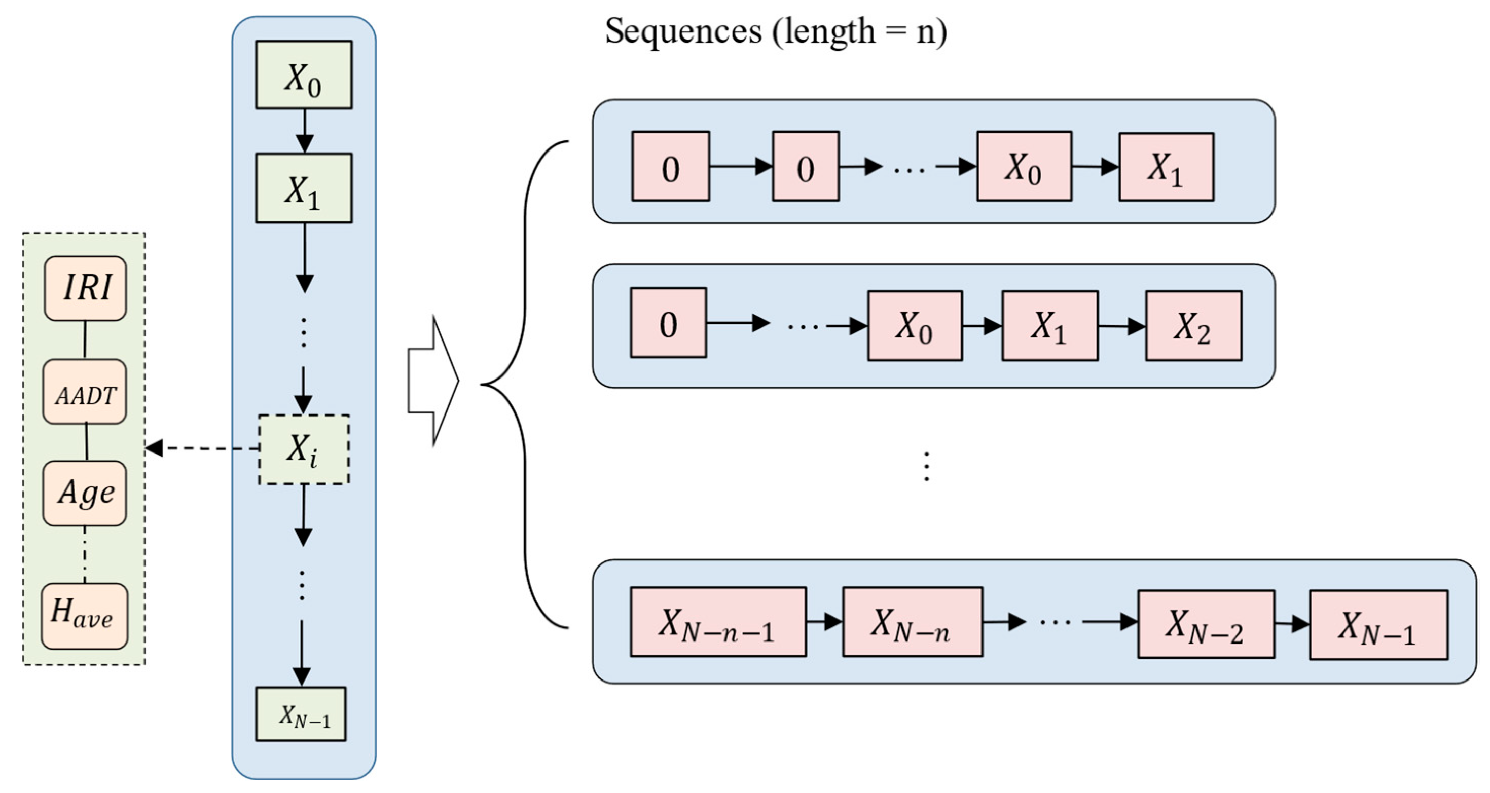
We transferred the data into sequences, as is required by LSTM models. For a road with N-years of recordings, $\alpha =\left[X_0,X_1,\dots ,X_{N-1}\right]$, it would be divided into several sequences (where sequence length is $n$), rather than putting the whole recording $\alpha$ into the model. As shown in Figure 1, $N-1$ sequences would be generated from this road. Zero was padding as default if there were not enough recordings in a single sequence.

For example, if a road had five IRI measurements (through 2018 to 2022), four sequences would be generated with one, two, three, and four historical elements with the goals of predicting this road’s second, third, fourth, and fifth year’s IRI value, respectively. These sequences contain the initial measurements and are continuous. This method’s ability to process variable-length sequences makes it more flexible and adaptable to real-world pavement data, where the length of historical data may vary for different road sections. However, as many sequences are subsets of other sequences and in order to prevent data leakage, we separated our train and test datasets by which roads were in them, not by randomly splitting the samples. The samples are arranged in order of least recent to most recent. Every sample has a feature representing the number of months since the road was constructed to when the measurement was made. There is also an empty sample appended to the end of every sequence that contains only the number of months since the construction to predict the IRI.

We also transposed the original input matrix to increase the training speed and accuracy of our models as shown in Figure 2.

As one of the main problems with processing and predicting this kind of data are retaining the impact of inputs from earlier in the input sequence, transposing the input matrix allows the model to process the entire series of events at the same time. In the transposed data, the model is not given a sequence of events. It is given a series of properties that have only an implied sequence and an explicit temporal order for all the data points. This greatly reduces the requirements on the model to remember, and helps both models, like the RNN, which have problems with vanishing gradients, and models like LSTMs and the LSTM+MA, which already have other measures in place to help.

At the same time, some other preprocessing was applied to the data. The mean value of the left and right wheel path IRI was used as the IRI value of a road. Min–max scaling was applied to each parameter, which is particularly useful when the features have different scales or ranges, as it helps to normalize the data and bring all features to the same scale (0 to 1). It is commonly employed in machine learning algorithms that are sensitive to the scale of the input features.

2.3. LSTM+MA

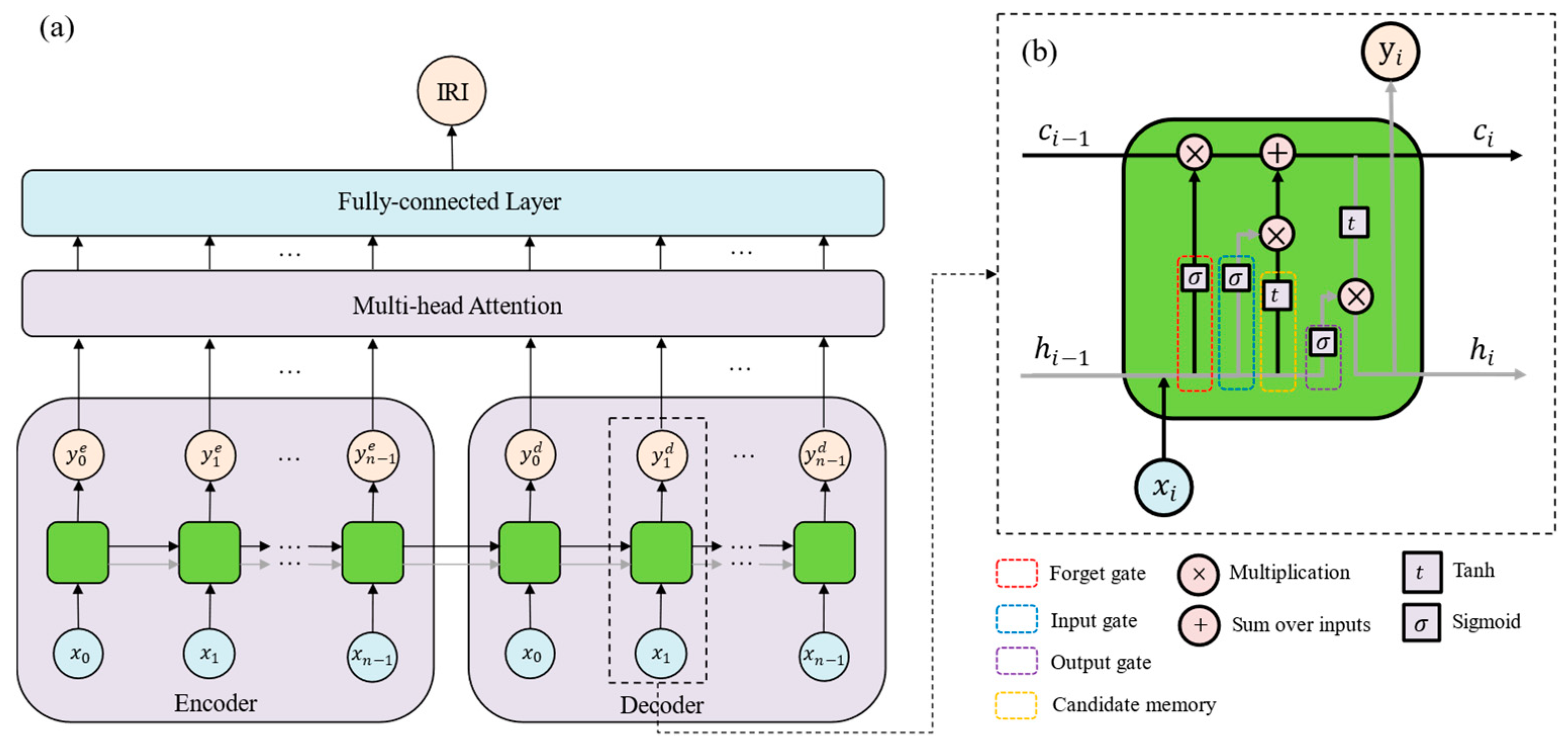
The proposed LSTM+MA model is a sequence-to-sequence architecture that combines LSTMs and attention mechanisms as shown in Figure 3. It is designed for predicting the IRI of pavement, and is based on various predictors from traffic, climate, pavement construction and maintenance.

The presented LSTM+MA follows an encoder–decoder architecture, which is commonly used for sequence-to-sequence tasks (Figure 3a). The encoder processes the input sequence $[{\mathit{x}}_{\mathbf{0}},{\mathit{x}}_{\mathbf{1}},\dots ,{\mathit{x}}_{\mathit{n}\mathbf{-}\mathbf{1}}]$ and captures its temporal information, while the decoder generates the output sequence $[{\mathit{y}}_{\mathbf{0}}^{\mathit{d}},{\mathit{y}}_{\mathbf{1}}^{\mathit{d}},\dots ,{\mathit{y}}_{\mathit{n}\mathbf{-}\mathbf{1}}^{\mathit{d}}]$, based on the information provided by the cell state ($c_i$) and the hidden state ($h_i$) from the encoder. LSTM is a type of RNN that addresses the vanishing gradient problem and allows for capturing long-term dependencies in sequential data [31]. The encoder and decoder both utilize LSTM layers, enabling the model to handle variable-length input and output sequences effectively. The LSTM component can be broken down into a few specific components that are responsible for different parts of the model’s behavior. The input gate, forget gate, output gate and candidate memory in the LSTM component can be explained using Equations (1)–(4).

$$i_i=\sigma ({\mathit{W}}_{\mathit{i}\mathit{i}}{\mathit{x}}_{\mathit{i}}+{\mathit{b}}_{\mathit{i}\mathit{i}}+{\mathit{W}}_{\mathit{h}\mathit{i}}{\mathit{h}}_{\mathit{i}-1}+{\mathit{b}}_{\mathit{h}\mathit{i}})$$

(1)

$$f_i=\sigma ({\mathit{W}}_{\mathit{f}\mathit{i}}{\mathit{x}}_{\mathit{i}}+{\mathit{b}}_{\mathit{f}\mathit{i}}+{\mathit{W}}_{\mathit{h}\mathit{f}}{\mathit{h}}_{\mathit{i}-1}+{\mathit{b}}_{\mathit{h}\mathit{f}})$$

(2)

$$o_i=\sigma ({\mathit{W}}_{\mathit{o}\mathit{i}}{\mathit{x}}_{\mathit{i}}+{\mathit{b}}_{\mathit{o}\mathit{i}}+{\mathit{W}}_{\mathit{h}\mathit{o}}{\mathit{h}}_{\mathit{i}-1}+{\mathit{b}}_{\mathit{h}\mathit{o}})$$

(3)

$$g_i=tanh ({\mathit{W}}_{\mathit{g}\mathit{i}}{\mathit{x}}_{\mathit{i}}+{\mathit{b}}_{\mathit{g}\mathit{i}}+{\mathit{W}}_{\mathit{h}\mathit{g}}{\mathit{h}}_{\mathit{i}-1}+{\mathit{b}}_{\mathit{h}\mathit{g}})$$

(4)

where $\sigma$ is the sigmoid function, tanh stands for the tangent hyperbolic function, $i_i$ is the input gate, $f_i$ is the forget gate, $o_i$ is the output gate, $g_i$ is the candidate memory, $\mathit{W}$ is the weight matrix and $\mathit{b}$ is the bias. The input, forget, and the candidate memory allow the model to learn what data to retain in the cell–matrix as it processes the sequence. The output gate updates the hidden state of the model. These components are then combined to generate the hidden and cell states, as shown in Equations (5) and (6).

$$h_i=o_{i }\odot tanh\left(c_i\right)$$

(5)

$$c_i=f_i\odot c_{i-1}+i_i\odot g_i$$

(6)

where $h_i$ is the output of the LSTM layer and the hidden layer for the next LSTM layer in the sequence. It can be calculated as the Hadamard product, or element-wise product of the output gate and the current cell state. $c_i$ is the current cell state and is the sum of the Hadamard product ($\odot$) of the forget gate and the last cell state, and the product of the input gate and the candidate gate. This step forgets old information and stores the new information that the model has. The Hadamard product multiplies corresponding elements of two matrices or vectors of the same dimension.

The attention mechanism enhances the model’s ability to focus on relevant parts of the input sequence when generating the output. This is especially useful in long sequences, as it helps the model to attend to the most informative time steps and ignore noise or less relevant information.

Multi-head attention [32] is used as the attention mechanism in this work because it allows the model to attend to different positions within the input sequence simultaneously. It computes multiple attention heads, each capturing different patterns and relationships in the data. Moreover, it helps the model capture complex dependencies and relationships between predictors, which can be valuable in pavement IRI prediction, where the performance is influenced by multiple factors. The attention mechanism embedded improves the model’s interpretability by highlighting the importance of different parts of the input sequence during the prediction process. After applying the attention mechanism, the model uses a fully connected layer to transform the output to the desired prediction format (IRI values). The output is reshaped to match the appropriate dimensions for the final prediction.

There are several inherent advantages of combining he LSTM and multi-head attention mechanisms in the proposed LSTM+MA model. Firstly, the LSTM layer is a specialized variant of RNNs, designed to address the vanishing gradient problem and facilitate the modeling of long-term dependencies in sequential data. By incorporating memory cells and gating mechanisms, LSTMs can effectively retain and update information over extended time steps, making them particularly well-suited for time series prediction tasks. The cell state ($c_i$) is controlled by the forget gate, input gate, and candidate memory for each time step. By applying element-wise multiplication to the forget gate and the previous cell state, the LSTM forgets irrelevant information. The input gate and the candidate memory determine which new information is incorporated into the updated cell state. The resulting cell state retains valuable historical context while selectively integrating new information, facilitating the modeling of long-term dependencies in the data. The hidden state ($h_i$) is the LSTM layer’s output for the current time step, representing the processed and summarized information that is passed to the next time step. It is calculated by applying element-wise multiplication to the cell state and the output of the output gate. The hidden state captures relevant information from the current input and retains valuable historical context from previous time steps, enabling the LSTM to carry forward essential features as it processes the sequence. Secondly, the integration of multi-head attention enhances the LSTM’s ability by allowing the model to focus on specific parts of the sequence that are most relevant to the prediction. While the LSTM captures the sequential dependencies, the attention mechanism enables the model to dynamically weigh the importance of different time steps and features, thereby improving its interpretability and predictive accuracy. This combination ensures that the model can handle both the temporal dynamics of the data and the complex interrelationships among predictors.

By combining these two methods, the LSTM+MA model achieves a balance between sequential memory and contextual focus. The LSTM component ensures that the model retains a robust understanding of historical trends, while the attention mechanism allows for a nuanced and targeted analysis of key features and time steps. This synergy leads to improved performance in predicting time-dependent variables like pavement roughness, as it can effectively learn from both long-term dependencies and diverse feature relationships within the dataset.

2.4. Evaluation Metrics

The performance of models is evaluated by MSE and $R^2$. MSE measures the average of the squared differences between the predicted results and actual values. It can provide a measure of how well the model’s predictions align with the true values, with higher values indicating greater errors. It can be calculated using Equation (7).

$$MSE={\displaystyle \frac{1}{n}}{\sum }_{i=1}^n(y_i-{\widehat{y}}_i)$$

(7)

where n is the number of total evaluated data, $y_i$ is the i-th data point, ${\widehat{y}}_i$ is the prediction of the i-th data.

$R^2$ stands for the coefficient of determination. It measures the proportion of the total variation in the prediction that can be explained by the model. It is used to measure the accuracy of a model’s fit, and can be calculated using Equation (8).

$$R^2={\displaystyle \frac{SSR}{SST}}={\displaystyle \frac{\sum _{i=1}^n({\widehat{y}}_i-\overline{y})}{\sum _{i=1}^n(y_i-\overline{y})}}$$

(8)

where SSR is the sum of squares regression, SST stands for the sum of squares total, and $\overline{y}$ is the average value of the data.

To evaluate and compare the performance between different models statistically, each model is trained and tested three times on randomly split train and test datasets. The average value and standard deviation would be calculated, based on these tests. By performing this, the average value can show the general accuracy of the model while the standard deviation from different tests can represent the robustness of the model.

Overfitting problems are also considered in this work. Overfitting occurs when the regression models learn the training data too well, resulting in poor generalization to unseen data. The difference between the training and testing performance is considered as an overfitting score in this work as shown in Equation (9). It is utilized as a metric to quantify the overfitting issue in the selected approach.

$$S_o=R_{train}^2-R_{test}^2$$

(9)

where $S_o$ stands for the overfitting score, $R_{train}^2$ is the $R^2$ value when model is applied in the train set, $R_{test}^2$ is the $R^2$ value when model is applied in the test set. Its practical implication lies in quantifying the degree of overfitting in a straightforward and interpretable way. A larger $S_o$ indicates a greater disparity between the training and testing performance, signaling that the model may be overfitting to the training data and struggling to generalize to unseen data. Conversely, a smaller $S_o$ reflects better generalization and indicates that the model is learning meaningful patterns rather than memorizing the training data.

2.5. Overall Procedure

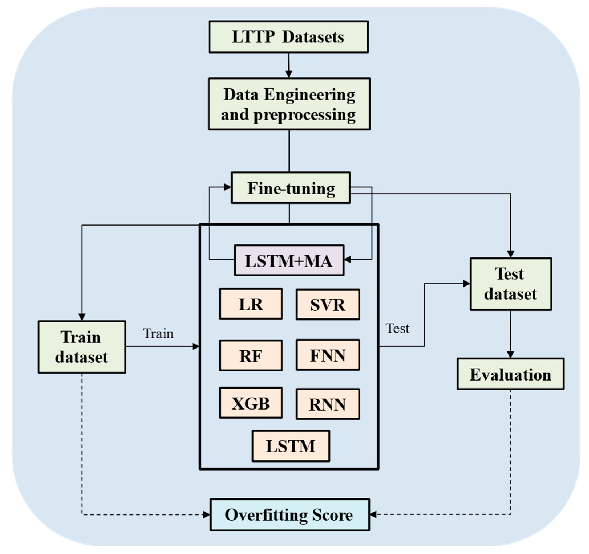
The aim of the work is to propose a model that can predict the IRI value with higher accuracy, based on the predictors extracted from the LTPP dataset. First, data engineering was applied on the LTPP data to seek some useful and related predictors for the IRI prediction. Then, data preprocessing was applied to process the data. The proposed model LSTM+MA was compared with other state-of-the-art models to show its high performance as shown in Figure 4. In this work, we chose not to use a separate validation dataset, due to the limited amount of independent data available, despite having 25,167 samples. These samples are derived from only 1026 unique roads, meaning that there are effectively 1026 independent data sequences after transforming the data into sequences. Splitting the dataset further to create a validation set would have significantly reduced the size of both the training and testing datasets, potentially compromising the model’s ability to learn effectively from the available data.

Seven models, which are popular used in other research, were trained and tested on this dataset and compared with our proposed method. The models included LR, SVR, RF, KNR, FNN, XGB, RNN and LSTM. The details of these models are shown in

Table 2. The description of all the models used in this work to compare with. SL stands for supervised learning, EL stands for ensemble learning, and ANN stands for artificial neural network.

Model	Type	Description
LR	SL	Logistic regression models the probability of an input belonging to a particular class using a logistic (sigmoid) function.
SVR	SL	An extension of support vector machines (SVM) for regression, where it tries to find a hyperplane that best fits the data, while minimizing the error.
RF	EL	Random forest is based on the concept of constructing multiple decision trees during training, and then combines their predictions to make a final prediction.
KNR	SL	KNN regressor is a non-parametric supervised learning algorithm used for regression tasks.
FNN	ANN	A feedforward neural network is an artificial neural network that consists of a series of linear layers.
XGB	EL	A variant of gradient boosting that builds multiple weak learners (often decision trees) sequentially, where each new learner corrects the errors made by the previous ones.
RNN	ANN	RNN is a type of neural network designed to handle sequential data, making it suitable for time-series analysis. Unlike traditional feedforward neural networks, RNNs have connections that form cycles, allowing them to maintain hidden states and process sequences of data.

. Each model would be run three times, based on a different train–test split. By performing this, the average and standard deviation of these three running could be calculated, which can make the experiments statistically meaningful. A hyperparameter fine-tuning process would be conducted in the LSTM+MA model to find the best performance it can reach. In this approach, the possible parameters, including the input sequence length, the learning rates, the learning rate decay rate, the LSTM layer dropout, the number of LSTM layers, the batch size, and the number of training epochs, are selected to determine the optimal permutation of input parameters for the model’s performance.

Machine learning models are implemented using Scikit-learn and PyTorch, two machine learning libraries in Python 3.8. The data processing methods and models are all implemented in Python and computed under the following machine speculations: Ubuntu 22.04.2 LTS, AMD Ryzen 9 5900, NVIDIA RTX 3080 with 16GB RAM, and 16GB of system RAM.

3. Results

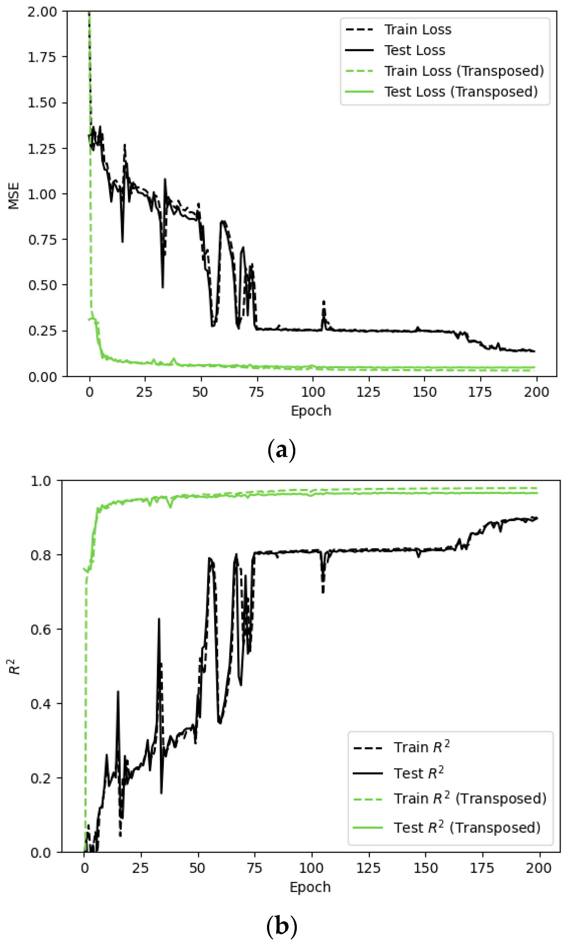
Figure 5 shows the difference in MSE and $R^2$ score during the training and testing procedure when using original dataset and the transposed dataset for the model LSTM+MA.

This shows that, no matter whether using original data or the transposed dataset, the predicting MSE is decreasing with the increasing of running epochs and the $R^2$ score increases with more running iterations. However, when the transposed and original time-series datasets are compared by training models with each dataset and looking at the MSE and $R^2$ over the training sequence, it can be seen that the transposed data leads to a significant improvement in training time and accuracy as shown in Figure 5. By utilizing the transposed data, the MSE drops dramatically and quickly to a very low state around epoch 25 which is even lower than the model in epoch 200 when using original data. In other words, the model learns from the data much more quickly when the LTPP data are transposed. Moreover, the method with transposed data as preprocessing performs much smoother in MSE and $R^2$. The model trained on the original data shows a sawtooth shape on the relationship between MSE (or $R^2$) with epochs. It means the model cannot learn very stably from the original data.

It is interesting to find that the test data closely mirrored the performance of the models on the training data no matter using original dataset or processed dataset, which means that the model demonstrates robustness to noise and generalizes well for unseen data.

After preprocessing the data, a grid-search approach is utilized to determine the optimal parameters for the LSTM+MA model. The input sequence length, the learning rates, the leaning rate decay, the LSTM layer dropout, the number of LSTM layers, the batch size, and the number of training epochs were selected to be optimized. We discovered that the optimal sequence length for the LSTM-MA model is five elements, and the optimal number of hidden layers for the encoder and decoder is three. The optimal parameters from the hyperparameter tuning are shown in

Table 3. Hyperparameter tuning results.

Parameter Name	Value
Learning rate	0.01
Number of hidden layers	3
Input sequence length	5
Learning rate decay	0.8
Batch size	512
Epochs	200
Dropout	0.25

.

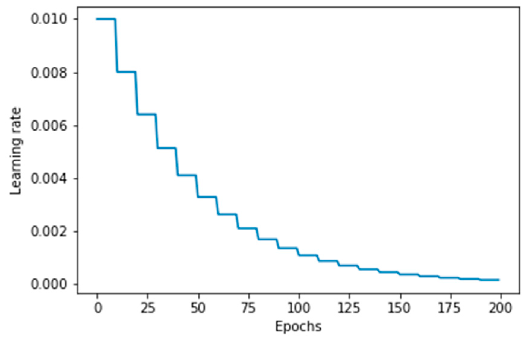
While the initial learning rate is set to 0.01, the model implements a learning rate decay mechanism (learning rate decay is 0.8) to address potential issues of stagnation or instability. This ensures that the learning rate starts at 0.01 to allow for rapid initial convergence, and then decreases gradually as training progresses, enabling more fine-tuned updates as the model approaches an optimal solution.

Figure 6 shows the learning rate change during training. The final learning rate depends on the total number of training steps. This dynamic adjustment balances efficient learning in the early stages with stability during later stages of training.

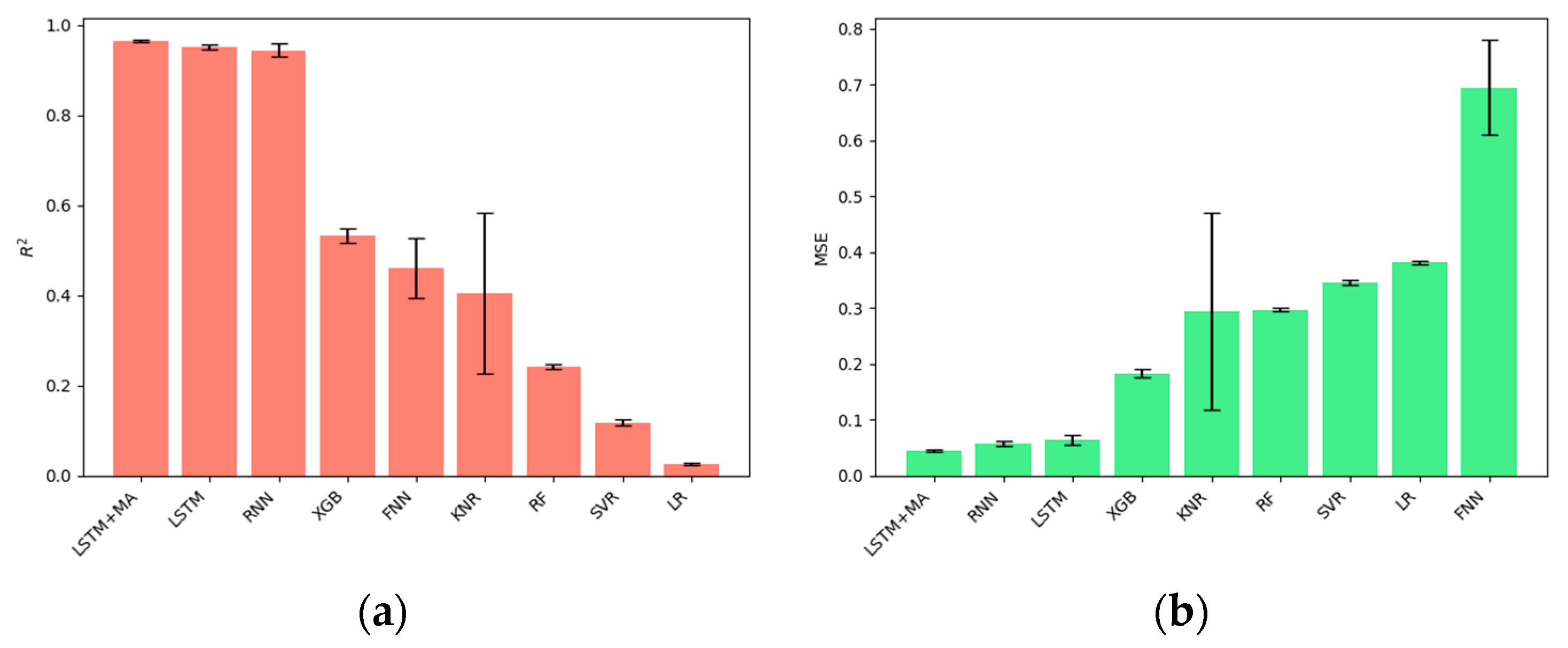
After determining the best performance of our proposed model, we compare this model to other state-of-the-art models, including LR, SVR, RF, KNR, FNN, XGB, RNN, and LSTM. Figure 6 shows the $R^2$ and MSE values from the models’ comparison results.

Figure 7a is organized in ascending order by the $R^2$ value of each model achieved on the test dataset. It shows that our proposed LSTM+MA model outperforms other models in the LTPP dataset, as it achieves the highest $R^2$ value (0.965) and the lowest MSE (0.030). It is noteworthy that the models which consider impacts over time, including RNN, LSTM, and LSTM+MA, have a higher accuracy than the models which do not consider the time-accumulated influence. The high performance of RNN, LSTM, and LSTM+MA proves that the pavement IRI is a time-dependent factor, and using a time-series model can perform better for IRI prediction. The black error bar is the standard deviation calculated by running models in randomly split train–test datasets. A small standard deviation means that the model performs stable in different data inputs. In other words, it can represent the robustness of the model. It is interesting to find that the KNR achieves the apparent larger standard deviation than other models, both in $R^2$ and in MSE, as shown in Figure 7. This is because the KNR algorithm is predicted based on the K nearest points, which means that it is highly related to the interaction among the data points. Our proposed model achieves the lowest standard deviation (0.0026) in $R^2$ value, which means it obtains a stable performance and is much more robust than other models.

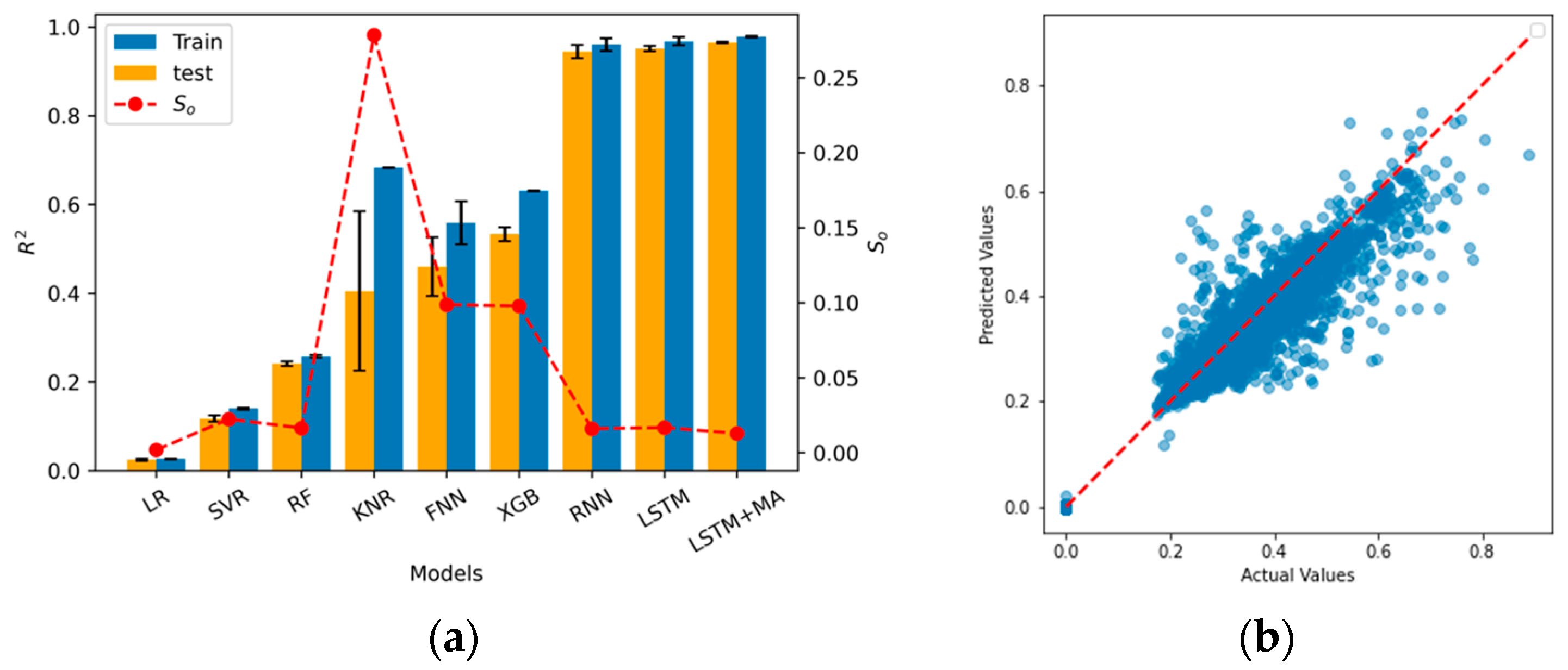
Overfitting is a serious problem in the long-term pavement performance prediction. It occurs when the model learns the training data too well, resulting in poor generalization. Therefore, to obtain the performance difference in the train and test dataset of each model, the $R^2$ score from the training and testing performance are considered and shown in Figure 8a. The red dash line represents the overfitting score ($S_o$) among all the models. It shows that KNR is the most overfitted model compared to others. Although LR obtains the lowest overfitting problem, with a $S_o$ of 0.0018, the performance of the LR model is the worst among all the models. The LSTM+MA achieves the second lowest $S_o$ (0.0128) except LR, and at the same time, it obtains the highest $R^2$ value. In other words, our proposed model retains a high accuracy, as well as a low overfitting problem, in predicting the IRI value, based on the LTPP dataset. Figure 8b shows the comparison between the ground truth data and model predictions from the proposed model. The alignment of the prediction results with the original data demonstrate the model’s accuracy and ability to capture the underlying patterns effectively.

4. Discussion

The proposed LSTM+MA, model adjusting the LSTM to make it combine with multi-head attention, reaches the highest $R^2$ value compared to other models. It leads to a higher performance than using a plain LSTM, which means that the embedded attention mechanism does improve the model information extraction and interpretation capacity.

The model that can handle time-series data shows a more dominant performance than other models. This is because the pavement IRI, as well as friction, rutting and deflection, are all time-series data, which means that the traffic, climate, and other factors would have an accumulated influence on these performances over time. In other words, our presented model is not only limited in predicting the pavement IRI, but also can be used to predict other pavement performance including the friction, deflection, and transverse profile, as they are all time-series data. Moreover, it can also be used in other fields like stoke price predicting or weather prediction where the data are highly time-related.

Although there are important improvements revealed by this study, there are also limitations. First, the choice of predictors were not considered thoroughly. We must point out that we did not discuss the dependency between each predictor which might introduce redundancy and overfitting into the model. However, these problems could be solved if we consider using a feature/component ablation section to choose the most related predictors. Also, we could apply principal component analysis (PCA) to reduce the dimensionality of data to avoid noise and redundancy. In the future study, the early stopping would be applied during the training to prevent the model from overfitting and save computational resources. We also plan to extend our study by including benchmark comparisons with advanced time-series models, like the temporal fusion transformer (TFT) to understand the relative strengths and weaknesses of LSTM-MA. This will involve applying both models to datasets of varying sizes to assess their performance under different data availability scenarios.

5. Conclusions

A LSTM-based model, LSTM+MA, is proposed in this work to predict the pavement IRI, based on time-series data extracted from the LTPP database. Traffic, climate, pavement construction, and maintenance are considered as the most important factors to the contribution of IRI, and are utilized as predictors to train the models. The original data are transferred to sequences first in order to improve usage of data in the model. The transformation of data into sequences and preprocessing techniques, like data transposition and scaling, are employed to optimize the model’s performance.

The presented LSTM+MA model was developed to address the limitations in existing methods, such as linear regression and traditional machine learning approaches, including LR, SVR, RF, KNR, FNN, and XGB, which fail to account for the time-dependent characteristics of pavement roughness. These existing approaches often lack the ability to capture long-term dependencies in data, resulting in limited predictive capabilities. By incorporating a sequence-to-sequence architecture using LSTMs with multi-head attention, the proposed model effectively addresses these challenges and improves predictive accuracy, while avoiding issues such as vanishing gradients.

The proposed model is designed for practical use in transportation infrastructure management. Specifically, it can aid transportation agencies in predicting pavement IRI over time, which is critical for decision-making in road maintenance and rehabilitation planning. The model is particularly suitable for applications in intelligent transportation systems, where precise predictions of time-dependent indices like IRI are necessary for efficient resource allocation and operational management.

The practical benefits of the model are significant. It obtains the highest $R^2$ value (0.965) and the lowest MSE (0.030) compared to other state-of-the-art models, demonstrating superior accuracy and robustness. The preprocessing methods and architecture of the model enable faster learning and convergence, making it efficient for real-time or large-scale applications. Furthermore, its design is versatile and can be adapted for predicting other time-dependent pavement performance indices, such as friction, deflection, and rutting. It also has potential applications in other fields where time-series data are crucial, including stock price forecasting and weather prediction.

However, the model does have limitations that need to be considered for a balanced perspective. For example, the interpretability of LSTM+MA remains a challenge, which might make it difficult for decision-makers to fully understand how specific predictors influence the output.

Our work primarily addresses the challenge of accurately predicting the time-dependent evolution of pavement indices, such as IRI, which are influenced by deterioration and maintenance interventions. The code and data are available at https://github.com/tjboise/RNN (accessed on 20 December 2024). While this study presents significant improvements in modeling IRI, future research could focus on expanding predictor selection, evaluating dependencies among predictors, and applying dimensionality reduction techniques to further optimize the model’s performance and applicability.