An Application of Reinforcement Learning to the Optimal Design of Road Vehicle Suspension Systems

Abstract

This study investigates the application of Multi-Objective Reinforcement Learning–Dominance-Based (MORL–DB) method to the optimal design of complex mechanical systems. The MORL–DB method employs a Deep Deterministic Policy Gradient (DDPG) agent to identify the optimal solutions of the multi-objective problem. By adopting the k-optimality metric, which introduces an optimality ranking within the Pareto-optimal set of solutions, a final design solution can be chosen more easily, especially when considering a large number of objective functions. The method is successfully applied to the elasto-kinematic optimisation of a double wishbone suspension system, featuring a multi-body model in ADAMS Car. This complex design task includes 30 design variables and 14 objective functions. The MORL–DB method is compared with two other approaches: the Moving Spheres (MS) method, specifically developed for spatial design tasks, and the genetic algorithm with k-optimality-based sorting (KEMOGA). Comparative results show that the MORL–DB method achieves solutions of higher optimality while requiring significantly fewer objective function evaluations. The results demonstrate that the MORL–DB method is a promising and sample-efficient alternative for multi-objective optimisation, particularly in problems involving high-dimensional design spaces and expensive objective function evaluations.

1. Introduction

The optimal design of complex mechanical systems typically involves a large number of design variables [1]. The advent of computer experiments [2], from the second half of the 20th century onwards, has greatly expanded the possibility for designers to explore a wide range of system configurations. However, the number of design variables often becomes so large that an exhaustive exploration of all the possible design solutions is not feasible, even with the most powerful computer available to designers. To overcome this limitation, two complementary strategies can be pursued: reducing the computational time needed to evaluate the system behaviour or reducing the number of evaluations needed to identify an optimal solution.

The first strategy can be addressed by adopting a surrogate model of the system [3]. In this approach, the original validated model based on physical laws is replaced with a black box that approximates the relationship between the design variables and the objective functions of the physical system. The black box, referred to in this paper as the surrogate model or approximator, is calibrated on a limited number of simulations of the original physical model, which are employed to tune the model’s the parameters. Several types of approximators exist, such as polynomial models [4], Kriging techniques [2,5], and artificial neural networks. Thanks to their ability in capturing the performances of the system even in the presence of highly non-linear or multi-modal responses [1], artificial neural networks have been widely employed in the context of optimisation problems, particularly in fields such as structural optimisation [6], vehicle dynamics [7], and vehicle suspension optimisation [8].

Regarding the reduction in the number of objective function evaluations required to solve an optimisation problem, a key idea is to sample the design domain in regions where a high density of optimal solutions is expected. This can be achieved by focusing on a subregion of the whole design domain and progressively moving to other subregions on the basis of the optimal solutions identified in previous iterations [9,10]. Another option is to prioritise the solutions with higher fitness levels according to a prescribed optimality metric, as is commonly realised with evolutionary algorithms [11,12] and other meta-heuristic algorithms [13], such as Tabu Search [14], Particle Swarm Optimisation [15], and Ant Colony Optimisation [16]. However, all these multi-objective optimisation techniques lack a specific learning process based on the design solutions found [17], relying instead on stochastic rules to generate new design solutions [18]. Indeed, no inferential process is employed to estimate the optimality of new solutions [19]; rather, they are simply generated by recombining previously analysed solutions with the addition of a random component.

Reinforcement Learning (RL) algorithms, on the other hand, are specifically designed to learn a policy that maximises a reward on the basis of a set of prior observations. Despite the potential demonstrated by RL techniques in the context of Multi-objective Optimisation (MO), relatively few studies have been published in this area [20]. Zeng et al. [21] proposed two Multi-Objective Deep Reinforcement Learning models, the Multi-Objective Deep Deterministic Policy Gradient (MO-DDPG) and the Multi-Objective Deep Stochastic Policy Gradient (MO-DSPG). They applied these to the optimisation of a wind turbine blade profile and to several ZDT test problems [22], showing superior performance compared to well-established Non-dominated Sorting Genetic Algorithm (NSGA) methods [23]. Similarly, Yonekura et al. [24] addressed the optimal design of turbine blades adopting a Proximal Policy Optimization (PPO) algorithm based on the hyper-volume associated with the optimal design solutions [25].

Yang et al. [26] developed a Deep Q-Network (DQN) algorithm [27] grounded in Pareto optimality to address the cart pole control problem [28]. Seurin and Shirvan [29] applied several variants of their Pareto Envelope Augmented with Reinforcement Learning (PEARL) algorithm to DTLZ test problems [30], as well as to constrained test problems such as CDTLZ [31] and CPT [32]. They compared their performance with NSGA-II [33], NSGA-III [34], Tabu Search [14], and Simulated Annealing [35]. After demonstrating the advantages of their method over these state-of-the-art algorithms, PEARL was applied to the constrained multi-objective optimisation of a pressurised water reactor.

Regarding different techniques, Ebrie and Kim [36] adopted a multi-agent DQN algorithm for the optimal scheduling of a power plant. Similarly, Kupwiwat et al. [37] employed a multi-agent DDPG algorithm to address the optimal design of a truss structure. The work of Somayaji NS and Li [38] introduced a DQN algorithm with a modified version of the Bellman equation [39] to handle multi-objective optimisation problems, applying it to the optimal design of electronic circuits. Importantly, this study also highlights the use of the trained agent in an inference phase, where it can be queried after training to identify new optimal solutions. Finally, Sato and Watanabe [40] faced a mixed-integer problem concerning the optimal multi-objective design of induction motors, proposing a method called the Design Search Tree-based Automatic design Method (DeSearTAM).

Besides the dimensionality of the design space, challenges in the optimisation of complex mechanical systems also arise from the need to consider a large number of objective functions. As this number increases, the fraction of non-dominated entries within the solutions set increases rapidly [41,42], making the Pareto optimality criterion alone insufficient to select a preferred design. To address this issue, Levi et al. proposed the concepts of k-optimality [43] and $k\epsilon$-optimality [44], which enable a further ranking among Pareto-optimal solutions.

Building on these challenges, this work explores an RL-based method for the multi-objective optimisation of complex mechanical systems with a high number of objective functions and compares its performance against state-of-the-art approaches. The specific method considered, called Multi-Objective Reinforcement Learning–Dominance-Based (MORL–DB) [20] employs a DDPG algorithm to explore the design space with the aim of increasing the k-optimality level of the solutions. Unlike DQN-based algorithms, designed for discrete action spaces [26,36,38], the adoption of a DDPG agent allows the MORL–DB method to effectively explore high-dimensional continuous design spaces [21]. In addition, differently from other multi-objective RL approaches in the literature [21,24,26,29,36,37,38,40], the MORL–DB method defines the reward function based on the k-optimality metric. This feature enables the method to successfully address many-objective optimisation problems, where Pareto optimality alone is not an effective selection criterion.

A proof of the effectiveness of the MORL–DB method has already been discussed by De Santanna et al. [45], who applied the algorithm to the optimisation of the elasto-kinematic behaviour of a MacPherson suspension system. In the present work, the MORL–DB method was applied to the optimal elasto-kinematic design of a double wishbone suspension system, modelled as a multi-body system in the ADAMS Car suite. The optimisation problem involves 30 design variables, including the coordinates of 8 suspension hard points and 6 scaling factors acting on the elastic characteristics of 2 of the suspension’s rubber bushings. These variables are constrained by the available three-dimensional design space for the hard point locations and by upper and lower bounds on the scaling factors. A total of 14 objective functions are considered.

This paper is structured as follows. The formulation of the multi-objective optimisation problem is presented in Section 1.1, together with the optimality metric adopted. In particular, the limitations of Pareto optimality in many-objective scenarios are discussed; then, the k-optimality metric is introduced as a more effective selection criterion. Section 1.2 provides a brief introduction to Reinforcement Learning, with a specific focus on the algorithm adopted in this study. Section 2 describes the MORL–DB method, while Section 3 illustrates the case study to which it is applied. Section 4 presents the results of the optimisation procedure, alongside those obtained through the MS method [9] and KEMOGA [44], which are compared in Section 5. Finally, Section 6 highlights the main findings of the present work and outlines possible directions for further research.

1.1. Multi-Objective Optimisation

Most of the engineering design problems typically require the minimisation of a set of objective functions. As a result, an optimal design problem is usually a multi-objective optimisation problem (MOP). A multi-objective optimisation problem with m objective functions and n design variables is defined as [1]

$$\begin{array}{c}\underset{\mathit{x}\in {\mathbb{R}}^n}{min}\mathit{f}\left(\mathit{x}\right):{\mathbb{R}}^n\to {\mathbb{R}}^m\hfill \\ \mathrm{subject}\mathrm{to}\hfill \\ g_i\left(\mathit{x}\right)\le 0i\in \left[1,q\right]\hfill \\ {\mathit{x}}_{lb}\le \mathit{x}\le {\mathit{x}}_{ub}\hfill \end{array}$$

(1)

where $\mathit{x}$ is the vector of the design variables (bounded between ${\mathit{x}}_{lb}$ and ${\mathit{x}}_{ub}$), $\mathit{f}\left(\mathit{x}\right)$ is the vector of the objective functions, and $g_i$ is one of the q design constraints. A feasible solution of the MOP is defined as a set of objective function values $\in {\mathbb{R}}^m$, obtained by evaluating the function $\mathit{f}$ at a vector of design variables $\mathit{x}\in {\mathbb{R}}^n$ that satisfies the given constraints. When compared with other feasible solutions, it may either dominate or be dominated [1]. Referring to a minimisation problem, a solution ${\mathit{x}}_i$ of the MOP is Pareto-optimal if $\nexists {\mathit{x}}_j$ such that [1]

$$\left\{\begin{array}{cccc}\hfill f_k\left({\mathit{x}}_j\right)& \le & f_k\left({\mathit{x}}_i\right)\hfill & \forall k\in \left[1,m\right]\hfill \\ \hfill \exists l:f_l\left({\mathit{x}}_j\right)& <& f_l\left({\mathit{x}}_i\right)\hfill \end{array}\right.$$

(2)

In other words, given a Pareto-optimal solution, it is not possible to find another solution improving at least one objective function without worsening at least another one. The Pareto-optimal solution set is called the Pareto-optimal set or Pareto front.

k-Optimality

Pareto optimality is easily achieved using design solutions that perform well in at least one objective function. As the number of objective functions increases, a growing fraction of solutions tends to be non-dominated in at least one objective function, leading to an inflation of the Pareto front. In practice, this means that in high-dimensional objective spaces, most solutions become Pareto-optimal, thereby reducing the effectiveness of Pareto dominance as a selection criterion.

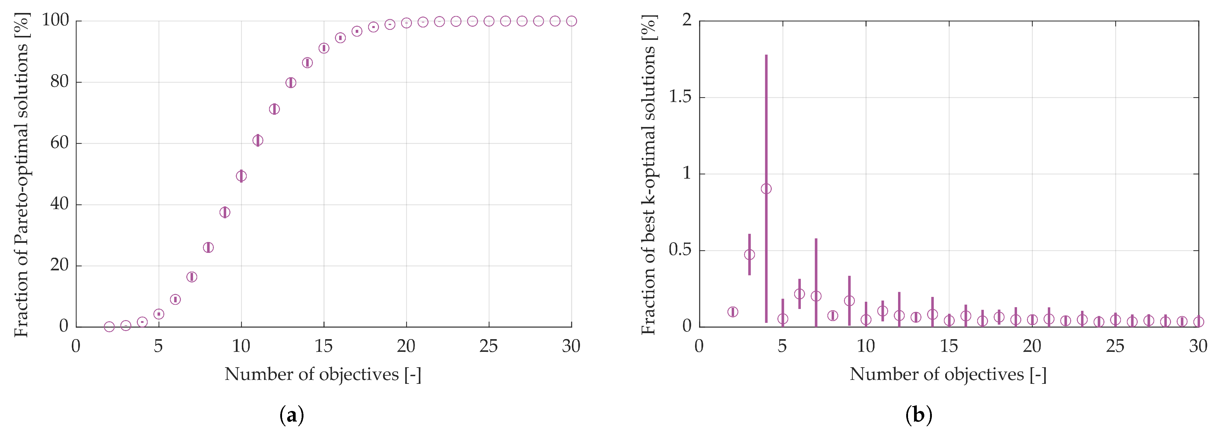
To illustrate this phenomenon, a randomised experimental setup was implemented to evaluate how the fraction of Pareto-optimal solutions evolves with the number of objectives. Each experiment is represented by a matrix in ${\mathbb{R}}^{10,000\times m}$, where each of the 10,000 rows corresponds to a randomly generated design solution and each of the m columns corresponds to an objective function. The entries of each matrix were independently sampled from a uniform distribution in the range $[0,10]$. For each value of m, ranging from 2 to 30, 1000 independent matrices were generated. For each matrix, the set of Pareto-optimal solutions was computed, and the fraction of these solutions relative to the total number of solutions in the matrix was calculated.

Figure 1 presents the results of this analysis. In Figure 1a, the average fraction of Pareto-optimal solutions is plotted against the number of objective functions m, with vertical segments indicating the corresponding standard deviation. The results clearly show that as the number of objective functions increases, the relative size of the Pareto-optimal set approaches the unity. This confirms that Pareto optimality alone, although useful to characterise non-dominated solutions, is insufficient to support the designer in selecting a final solution when dealing with many-objective optimisation problems [41].

To overcome this limitation, Levi et al. [43] propose the concept of k-optimality to rank Pareto-optimal solutions. Given the MOP of Equation (1), a solution is k-optimal if it is Pareto-optimal for any subset of $m-k$ objective functions. It follows that the optimality level k of a solution can vary from 0, for a simple Pareto-optimal solution, to $m-1$ for a solution that optimises all the objective functions of the problem. This latter case is the Utopia solution, which cannot be achieved in any well-posed MOP.

By definition, the optimality level k of a solution represents the maximum number of objective functions that it is possible to remove from the MOP without violating the its Pareto optimality condition. In contrast, a simple Pareto-optimal solution (i.e., $k=0$) may lose its dominance even if a single objective function is neglected [9]. Top-ranked k-optimal solutions are therefore characterised by the highest robustness in their Pareto optimality, as they are less sensitive to changes in the set of objective functions of the MOP. Moreover, as shown in Figure 1b, considering the fraction of top k-optimal solutions for the same experimental setup as in Figure 1a enables a much stricter selection of the final design solution. Unlike Pareto optimality, the proportion of top-ranked k-optimal solutions remains consistently low across all problem dimensions, which significantly reduces the set of alternatives and thus assists the designer, even in many-objective scenarios.

For an operative definition of the optimality level k of a solution [9], it is possible to consider a corollary [43] of the definition, which states that a k-optimal solution improves at least $k+1$ objectives over any other solution in the MOP. This allows for an efficient implementation in computer programming.

1.2. Reinforcement Learning

This section outlines the general framework of Reinforcement Learning (RL) and its adaptation to the context of multi-objective optimisation. Reinforcement Learning is an approach used to improve the performance of an artificial machine that interacts, performing some actions, with an environment. The core of RL lies in the feedback information passed through the reward function, a scalar function that measures the goodness of the new state of the environment after the machine perturbed it with its action. The artificial machine establishes the action to perform according to an inner policy that uses the state of the environment as information. The reward feedback mechanism constantly informs the machine on how good its past actions were. A training algorithm updates the policy of the machine to maximise the expected future rewards, that is, the rewards that the machine expects to receive for future actions. Figure 2 shows the general framework for RL, in which n is a generic step within the evolution of the environment E. The environment, described by its state $s_n$, is perturbed by the action $a_n$ and reaches the state $s_{n+1}$ because of it. Agent A is rewarded with the scalar function $r_n(s_n,a_n,s_{n+1})$, which is a judgment, in numerical terms, of the performed action. Then, the policy of the agent is updated using an internal training algorithm that aims to maximise the expected reward of future actions.  

Deep Deterministic Policy Gradient

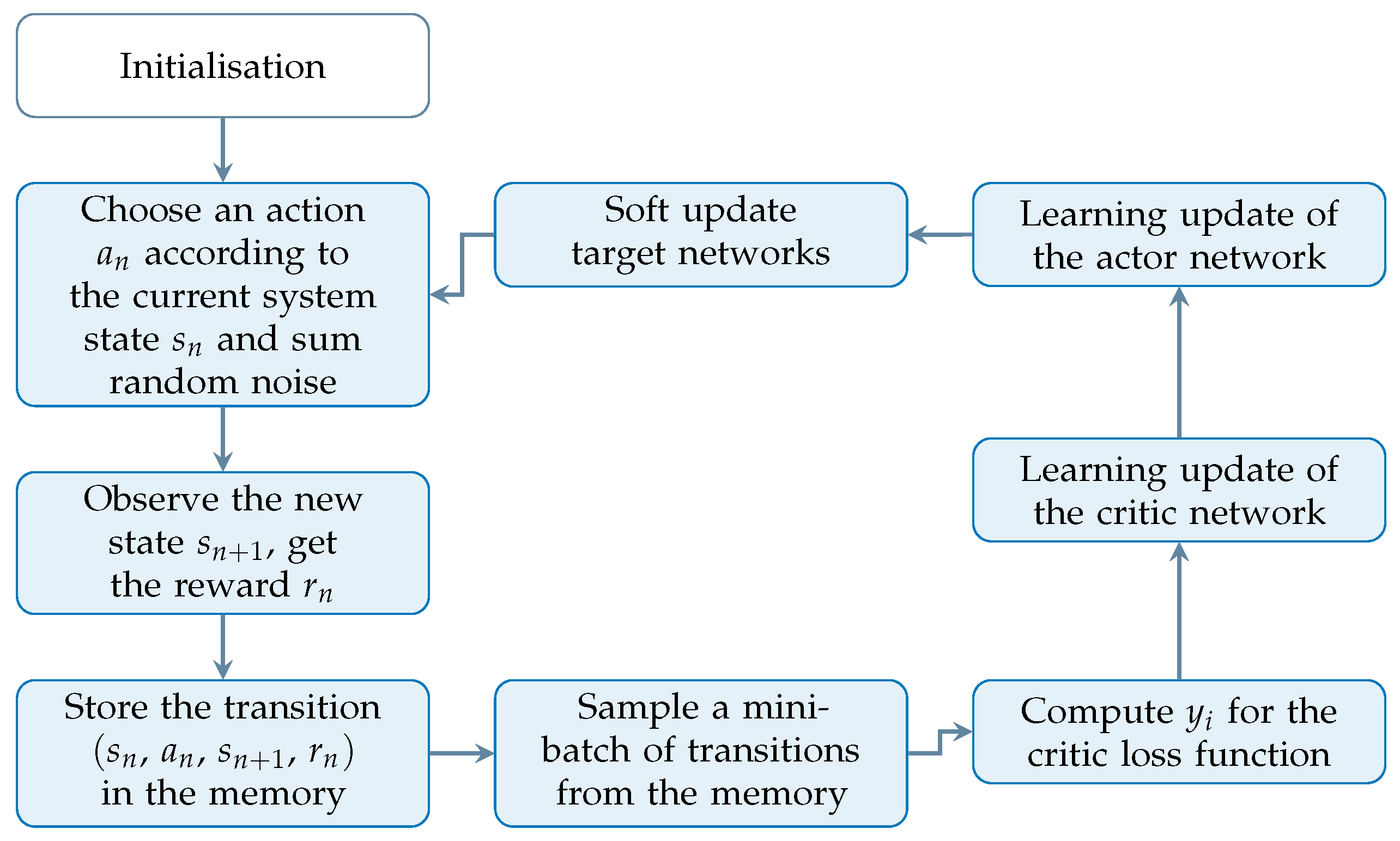
The Deep Deterministic Policy Gradient (DDPG) is a model-free, off-policy, actor–critic algorithm that exploits deep neural networks to learn control strategies in high-dimensional, continuous action domains. This means that the DDPG operates without a predefined model of the environment (model-free), learns a target policy different from the one used to generate behaviour of the actor (off-policy), and relies on the interplay between two neural networks typically referred to as the actor and the critic. The DDPG combines ideas the from Deep Q-learning method [27], which is restricted to discrete action spaces, and the Deterministic Policy Gradient (DPG) method [20], which performs well generally but struggles with more complex control challenges. A summary of the algorithmic flow of the DDPG is presented in Figure 3.

The agent follows the results of the cooperation between two artificial neural networks, the actor and the critic. The actor is a neural network tasked with choosing an action based on the current environment state $s_n$. The function governing this decision is the policy $\pi$, which maps inputs from the state space to outputs in the action space, so that $a_n=\pi \left(s_n\right)$. Given a state $s_i$, an action $a_i$, and a reward $r_i$, the cumulative expected reward, discounted over future steps and obtained by following the policy $\pi$, is referred to as the expected return:

$$J\left(s_n\right)={\mathbb{E}}_{r_i,si+1,a_i}\left[\sum _{i=n}^N{\gamma }^{(i-n)}r(s_i,a_i,s_{i+1})\right]$$

(3)

Here, N denotes the number of future steps considered, and $\gamma \in [0,1]$ is a discount factor that adjusts the weight of future rewards. The objective in the DDPG is to derive an optimal deterministic policy $\mu \left(s_n\right)$ that maximises the expected return $J\left(s_n\right)$ from each state $s_n$.

The critic network estimates the action-value function $Q^{\pi }(s_n,a_n)$, commonly referred to as the Q-function. This function evaluates the quality of an action taken in a given state by calculating the expected cumulative reward starting from $(s_n,a_n)$ and continuing under policy $\pi$. For deterministic policies $\mu \left(s_n\right)$ used in the DDPG, the Q-function satisfies the following Bellman equation:

$$Q^{\mu }(s_n,a_n)={\mathbb{E}}_{r_n,sn+1\sim E}\left[r(s_n,a_n)+\gamma Q^{\mu }(s_{n+1},\mu \left(s_{n+1}\right))\right]$$

(4)

The critic, described by ${\Theta }^Q$, is trained to estimate the optimal Q-function corresponding to the optimal policy $\mu \left(s_n\right)$. Its training objective is to minimize the Mean Squared Bellman Error (MSBE), given by

$$L\left({\Theta }^Q\right)={\displaystyle \frac{1}{N}}\sum _i{(y_i-Q(s_i,a_i|{\Theta }^Q))}^2$$

(5)

The target values $y_i$ are obtained from the right-hand side of Equation (4) and are computed using a target actor ${\mu }^{\prime }\left(s_n\right|{\Theta }^{{\mu }^{\prime }})$ and a target critic $Q^{\prime }(s_n,a_n|{\Theta }^{Q^{\prime }})$, which enhance training stability:

$$y_i=r_i+\gamma Q^{\prime }(s_{i+1},{\mu }^{\prime }\left(s_{i+1}\right|{\Theta }^{{\mu }^{\prime }})|{\Theta }^{Q^{\prime }})$$

(6)

The actor is optimised to learn the policy $\mu \left(s_n\right)=\underset{a_n}{argmax}{Q}^{\mu }(s_n,a_n)$. Its parameters ${\Theta }^{\mu }$ are updated through the deterministic policy gradient, using mini-batches of randomly selected transitions:

$${\nabla }_{{\Theta }^{\mu }}J\approx {\displaystyle \frac{1}{N}}\sum _n{\nabla }_{a}Q(s_n,a|{\Theta }^Q){|}_{a=\mu \left(s_n\right)}\nabla {\Theta }^{\mu }\mu \left(s_n\right|{\Theta }^{\mu })$$

(7)

Rather than fully transferring the main networks’ weights to the target networks, DDPG performs soft updates to gradually adjust target parameters

$${\Theta }^{\prime }\leftarrow \tau \Theta +(1-\tau ){\Theta }^{\prime }$$

(8)

This mechanism ensures more stable learning by preventing abrupt changes in target values, especially when the coefficient $\tau$ is small.

To promote exploration and increase the probability of discovering high-performing policies, random noise sampled from a stochastic process $\mathcal{N}$ is added to the deterministic actor output. The resulting exploration policy $\tilde{\mu }\left(s_n\right)$ is

$$\tilde{\mu }\left(s_n\right)=\mu \left(s_n\right|{\Theta }^{\mu })+\mathcal{N}$$

(9)

Over the training episodes, the added noise is gradually reduced, making the policy more deterministic. In this study, uncorrelated, mean-zero Gaussian noise is used [46], with its standard deviation updated after each training episode as

$${\sigma }_{n+1}={\sigma }_n(1-D)$$

(10)

where ${\sigma }_{n+1}$ is the standard deviation for the upcoming episode, ${\sigma }_n$ is the value for the current episode, and D is a predefined decay factor. Training does not begin immediately: a warm-up phase is included, during which the agent selects random actions to populate the transitions buffer and explore the design space.

2. Method

This section describes the Multi-Objective Reinforcement Learning–Dominance-Based (MORL–DB) [20] method. Before discussing the method in detail, as in Section 2.5, key aspects of system modelling and performance evaluation are introduced.

2.1. System Model

In engineering applications, it is usually assumed that a mathematical model describing the relevant physical behaviour of the system can be derived [1]. Such a model enables designers to predict system responses for any given set of input parameters, thereby reducing the need for extensive experimental campaigns. Mathematical representations are typically grounded in the governing physical laws—such as Newtonian mechanics, thermodynamics, or fluid dynamics—depending on the nature of the system under study.

For mechanical systems, common modelling approaches include lumped parameter methods [47] and multi-body formulations [48]. In a multi-body framework, the system is idealised as an assembly of rigid and flexible bodies connected by joints, springs, dampers, or other elements representing elastic and dissipative behaviour [49]. Its kinematics are then governed by motion constraints imposed by these connections. While idealised joints and rigid bodies are often assumed, it is also possible to incorporate flexibility and non-linear effects to better approximate real-world dynamics.

2.2. Design Variables and Constraints

A mathematical model is generally described by a set of variables. The aim of optimal design is to find the optimal set of variables that defines the optimal configuration of the system [1]. In multi-objective and continuous problems, the number of optimal sets of variables, and therefore of optimal solutions, is infinite. The variables on which designer acts are referred to as design variables (DV).

Constraints are conditions that must be satisfied for a design solution to be feasible. A common constraint is imposed by lower and upper bounds on the design variables. These limits can be imposed by a volume, as the three-dimensional space available to allocate the hard points of an automotive suspension system [9]. Additional constraints may arise from physical limitations on the system behaviour.

2.3. Objective Function Computation

The behaviour of a system is described by a number of performance parameters, defined with respect to a specific set of criteria related to the design problem. These criteria form a basis called the set of criteria [1]. If the system’s performance can be mathematically expressed according to these criteria, they are referred to as objective functions (OFs). Objective functions are formulated as functions of the design variables and represent the quantities that the designer aims to optimise. In this work, as in most of the technical literature, optimisation is understood as the minimisation of the objective functions.

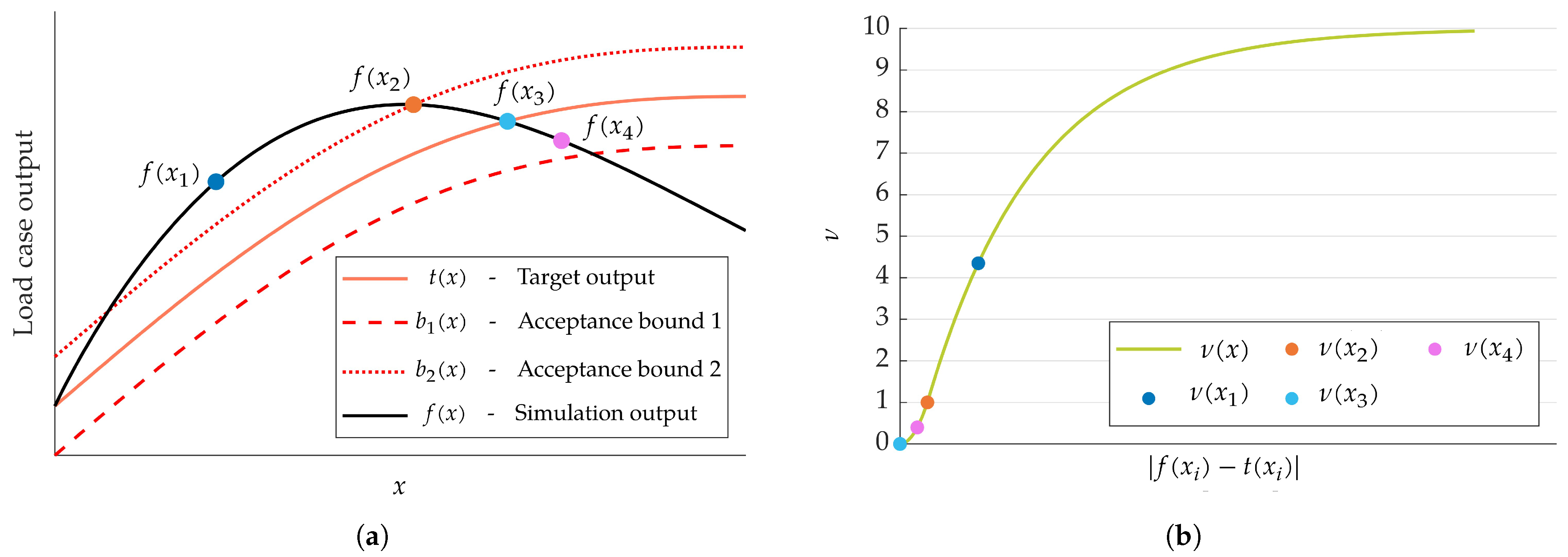
The case study considered in this work relies on multi-body simulations. An example of a multi-body output curve is shown in Figure 4a. The black line denotes the multi-body analysis output curve, while the red lines indicate the corresponding acceptance bounds, defined by the designer prior to optimisation. These bounds provide a reference for the computation of the objective function. When the output curve lies within them, the system performance is considered acceptable and the objective function assumes a low value. Conversely, output curves outside the bounds are penalised by higher objective function values, reflecting poorer compliance with respect to the target behaviour.

The output curves are assumed to be discretised into a number of points, hereinafter referred to as increments. The first step in computing the objective function is to assign a value $\nu \in \left[0,10\right)$ to each increment of the output curve. The envelope of the halfway points between the acceptance bounds defines a curve called the target. The value $\nu$ quantifies the deviation in each increment from the target. When the output lies exactly on the target, $\nu =0$, as the distance from the bounds increases indefinitely (in either direction), $\nu \to 10$. If an increment lies on one of the bounds, then $\nu =1$. Since the zero is defined symmetrically with respect to targets, the value of $\nu$ depends only on the magnitude of the deviation from the target and not on its sign. The value of $\nu$ is computed according to Equation (11):

$$\left\{\begin{array}{cc}\nu \left(x_i\right)={\left({\displaystyle \frac{f\left(x_i\right)-t\left(x_i\right)}{b_1\left(x_i\right)-t\left(x_i\right)}}\right)}^2\hfill & \mathrm{if}f\left(x_i\right)\in \left[b_1\left(x_i\right),b_2\left(x_i\right)\right]\hfill \\ \\ \nu \left(x_i\right)=10-9e^{-{\displaystyle \frac{|f\left(x_i\right)-b_{★}\left(x_i\right)|}{\lambda }}}\hfill & \mathrm{if}f\left(x_i\right)\notin \left[b_1\left(x_i\right),b_2\left(x_i\right)\right]\hfill \end{array}\right.$$

(11)

where $f\left(x_i\right)$ is the value of the multi-body output curve, $x_i$ is the value of the independent variable of the multi-body simulation, and $b_1\left(x\right)$ and $b_2\left(x\right)$, with $b_1\left(x\right)<b_2\left(x\right)\forall x$, are the acceptance bounds. The target value $t\left(x_i\right)$ is defined as

$$t\left(x_i\right):={\displaystyle \frac{b_1\left(x_i\right)+b_2\left(x_i\right)}{2}}$$

Note that when the increment is within the bounds, $\nu \left(x_i\right)$ is a squared normalised residual; otherwise, the value of $\nu$ grows according to a first-order exponential law. In particular, $b_{★}\left(x_i\right)$ denotes the closest bound to increment $f\left(x_i\right)$, defined as

$$b_{★}\left(x_i\right):=\underset{j=1,2}{argmin}\left|f\left(x_i\right)-b_j\left(x_i\right)\right|$$

while $\lambda$ is defined as $\lambda :=2·max\left|b_1\left(x_i\right)-b_2\left(x_i\right)\right|$. The trend of $\nu$ with respect to the distance from the target is shown in Figure 4b. Once all increments have been assigned a $\nu$ value, the objective function for the given multi-body output curve, here identified as $f_{OB}$, is computed as the arithmetic mean:

$$f_{OB}={\displaystyle \frac{1}{N}}\sum _{i=1}^N\nu \left(x_i\right)$$

(12)

where N is the total number of increments of the curve.

This procedure for computing an objective function from a curve is applicable to any kind of output, provided that acceptance bounds can be assigned and are meaningful for the problem at hand.

2.4. Surrogate Model

In some applications, the evaluation of the objective functions requires time-consuming simulations that significantly reduce the efficiency of the optimisation process. To address this, the physical model can be replaced with a surrogate model that approximates the system’s behaviour more quickly, enabling a more efficient exploration of the design space.

It should be noted that the use of a surrogate model is not an intrinsic component of the MORL–DB method [20], but rather an optional extension to be adopted when the computational complexity of the problem makes it advantageous.

2.5. Multi-Objective Reinforcement Learning–Dominance-Based (MORL–DB)

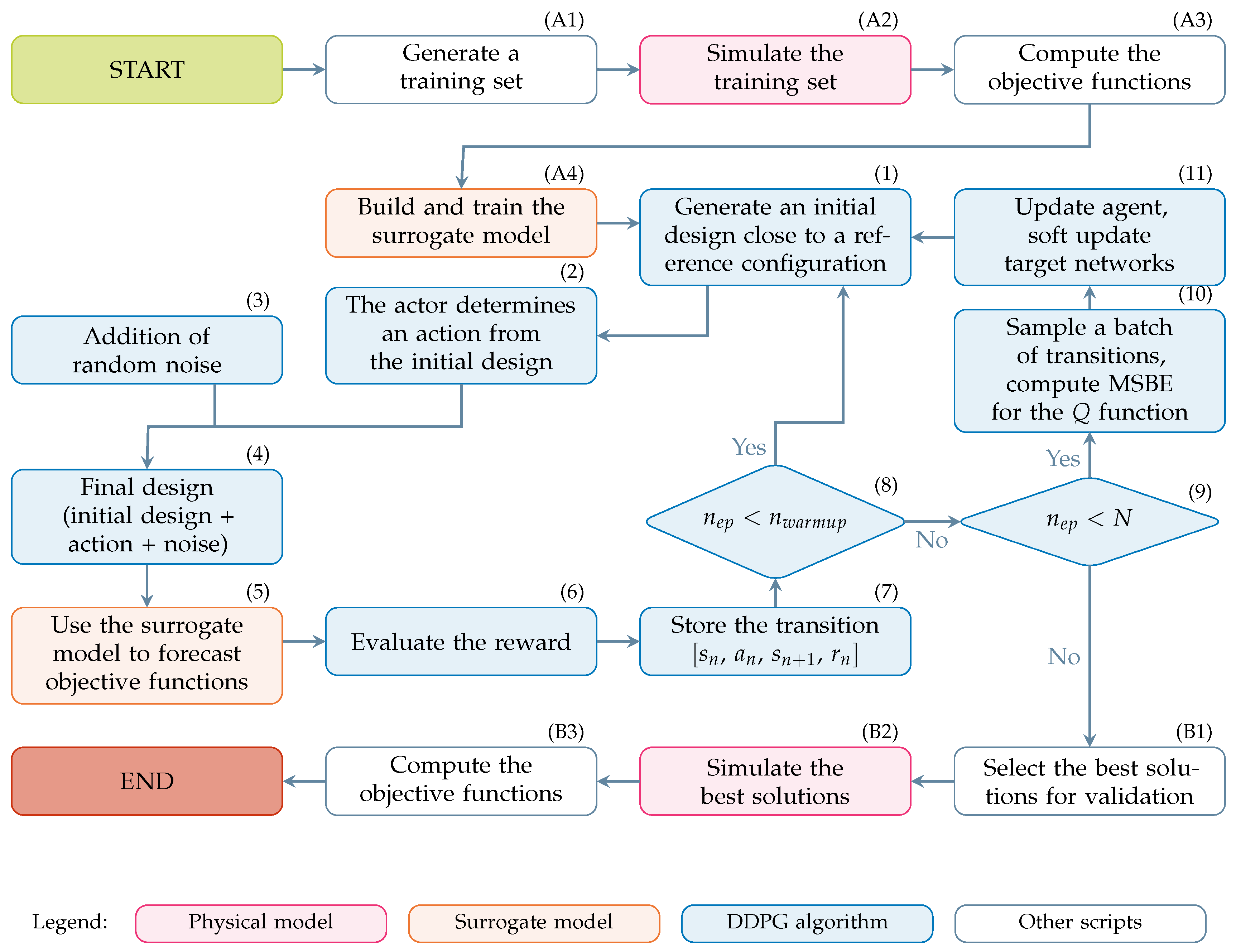
The complete workflow of the MORL–DB method is summarised in Figure 5 and consists of the phases listed below. The initial stage of surrogate model training–phases (A1)–(A4)–and the final validation stage–phases (B1)–(B3)–can be omitted when the optimisation is carried out directly on the physical model:

(A1) 

To train a surrogate model for the physical model, a training set must be generated to describe the behaviour of the environment. The training set is a collection of design solutions used to train the surrogate model. If the physical model is used instead, proceed directly to phase (1).

(A2) 

The training set is simulated to sample the system’s behaviour.

(A3) 

The objective functions of the training set (Section 2.3), together with the corresponding design variables, constitute the dataset used to train the surrogate model.

(A4) 

In this work, the system is approximated using feed-forward neural networks (FNNs), each with two hidden layers and a single output node. Each objective function is approximated with a distinct FNN. Having a different approximator for each objective function results in a better accuracy. The optimal number of neurons in the hidden layers is determined using a genetic algorithm. Candidate networks are evaluated through a fitness function that combines the coefficient of determination $R^2$ and the mean squared error between the training data and the approximation.

The fitness $FI{T}_{FNN}$ of each candidate network is computed as

$$FI{T}_{FNN}=1000·MSE-R^2+1,$$

(13)

where $MSE$ is the mean squared error between the training data and the approximation, and $R^2$ is the coefficient of determination, i.e., the quality of the linear regression between the training data and approximation.

(1) 

In optimal design, the system’s performance depends solely on its configuration, which is fully described by a set of design variables. In typical Reinforcement Learning settings, however, the reward is linked to a state transition (see Section 1.2). Accordingly, each iteration of the proposed method involves a design change, starting from an initial configuration and leading to a final one. Although the reward depends only on the final design, it is associated with the transition to enable proper training (see Figure 3). To enrich the diversity of explored solutions, the initial design solution is randomly sampled within a neighbourhood of a reference configuration. This also improves the sampling properties of the method, preventing the deterministic policy from converging to the same final design solution.

(2) 

In accordance with the policy at its disposal, the actor performs an action to modify the initial design variables set, randomly chosen, into a new set representing the final design solution. The actor operates with the aim of maximising the reward expected for its action, relying on experience gained from previous iterations.

(3) 

Uncorrelated mean-zero Gaussian noise is applied to the action to improve exploration efficiency in the DDPG algorithm. Noise is progressively reduced: it is required at the beginning to explore the design space, but would hinder a properly trained actor towards the end of the process.

(4) 

The final design solution is obtained by combining the initial design solution, the deterministic action of the actor, and the random noise.

(5) 

At this stage, the surrogate model is used to evaluate the performance of the final design solution in terms of objective functions. If a surrogate model is not used, the final design solution is processed through the physical model specific to the problem, and the objective functions are computed.

(6) 

As stated in phase (1), the reward depends only on the final design solution. In this work, it is set equal to the k-optimality level (see Section 1.1) of the final design solution relative to all solutions computed in previous iterations. The reward function can be customised for the problem at hand, e.g., by taking into account the violation of constraints or by adopting the Pareto optimality metric if a few objective functions are considered [20].

(7) 

The transition is stored in the state transition buffer. A transition includes the following:

The initial design solution—phase (1);

The action performed by the actor—phase (2);

The final design solution—phase (4);

The reward associated with the final design solution – phase (6).

(8) 

To ensure a sufficiently rich set of state transitions before the learning begins, the agent undergoes a prescribed number of warm up iterations. During this phase, the agent behaves erratically, as it is initialised with random weights and has not yet been trained.

(9) 

The MORL–DB method terminates after a given number of iterations are performed. The results are then validated as described in phase (B2) and the following.

(10) 

A batch of previously collected state transitions is randomly sampled from the replay buffer. These transitions are used to compute the Mean Squared Bellman Error (MSBE), which is minimised to update the critic network. This is possible because DDPG is an off-policy algorithm, allowing the reuse of transitions regardless of the current policy.

(11) 

The critic network is updated by minimising the MSBE, while the actor is updated using the deterministic policy gradient. To improve training stability, both target networks (actor and critic) are softly updated; that is, instead of being overwritten, their parameters are slowly adjusted toward those of the main networks.

(B1) 

Once training is complete, the final results are validated using the physical model to obtain the output curves. As this stage is typically time-consuming, only the most promising design solutions in terms of k-optimality should be selected.

(B2) 

The design solutions selected for validation are simulated.

(B3) 

Finally, the objective functions of the validated design solutions are computed.

3. Case Study: Multi-Objective Optimisation of a Double Wishbone Suspension

Multi-objective optimisation of suspension systems presents significant challenges due to the combination of high-dimensional design spaces and multiple objective functions [9]. In the context of elasto-kinematic optimisation using multi-body models, several contributions have been published. For instance, Țoțu and Cătălin [50] and Avi et al. [51] applied genetic algorithms to suspension optimisation. The former investigated a design space with 12 variables, corresponding to the coordinates of four suspension joints, and addressed three objectives: wheelbase variation, wheel track variation, and bump steer during vertical wheel travel. The latter extends the dimensionality to 24 design variables by considering eight hard points, and optimises nine performance indices, combined into a single scalar objective function through a weighted sum approach. Bagheri et al. [52] also employed a genetic algorithm (NSGA-II [33]), acting on the lateral and vertical positions of three hard points, to optimise three kinematic objectives under static conditions.

Among more recent contributions, Magri et al. [53] proposed a novel modelling strategy and compared its performance against Simscape multi-body models. Olschewski and Fang [54] instead introduced a kinematic equivalent model to investigate the influence of bushing stiffness on suspension behaviour. Finally, De Santanna et al. addressed the optimisation of a MacPherson suspension system with 9 objective functions and 21 design variables, adopting a structured strategy for exploring the design space [9] and considering an application of the MORL–DB method [45]. To the best of the authors’ knowledge, this is the first application of Reinforcement Learning techniques to the optimal design of suspension systems [55].

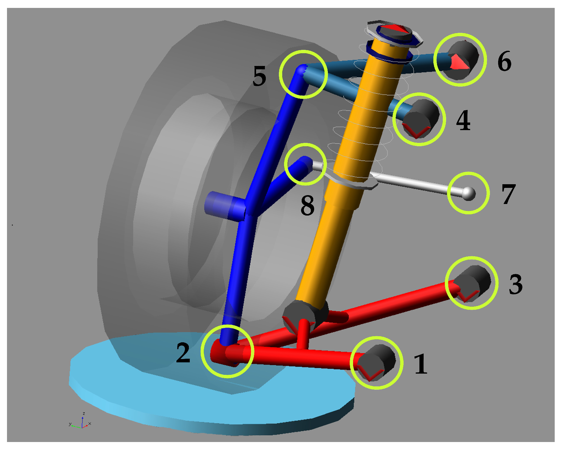
In this work, the Multi-Objective Reinforcement Learning–Dominance-Based (MORL–DB) method is applied to a case study related to the optimal elasto-kinematic design of a double wishbone suspension system, using a multi-body model available in the ADAMS Car suite (part of the acar_shared database, see Figure 6). The model is symmetric with respect to the vehicle’s vertical longitudinal plane, i.e., the plane normal to the y-axis of the reference system shown. All data presented in this work refer to the right-hand suspension; the left-hand suspension points share the same coordinates, except for a sign reversal in the y-coordinate. The system is optimised acting on 30 design variables: the three-dimensional coordinates of eight suspension hard points (HPs) and the values of six scaling factors (SFs), as summarised in

Table 1. The test case involves 30 design variables (DVs): spatial DVs are the three-dimensional coordinates of the hard points; elastic DVs are scaling factors acting on the bushings.

Design Variables (DVs)
Dimension of the design space 30
Spatial DVs 24	Elastic DVs 6

. The SFs modify the elastic behaviour of rubber bushings mounted at HP 1 and 3 by scaling their force–displacement curves along the force axis. Each bushing is associated with three independent SFs, scaling the elastic characteristics along three orthonormal directions, for a total of six design variables ascribed to bushings. A scaling factor greater than one increases stiffness, while a value below one reduces it.

All SFs have a nominal value of 1. Each hard point is allowed to move within a cubic design space with a side of 80 mm, centred on its nominal position (see

Table 2. Number (HP) and name (HP Name) of the suspension hard points involved in the optimisation. Nominal coordinates are expressed in mm. Numbers correspond to the identifiers of Figure 6.

HP	HP Name	x	y	z
1	lca_front	67	400	180
2	lca_outer	267	750	130
3	lca_rear	467	450	185
4	uca_front	367	450	555
5	uca_outer	307	675	555
6	uca_rear	517	490	560
7	tierod_inner	467	400	330
8	tierod_outer	417	750	330

). The scaling factors vary within the interval $[0.8,1.2]$, corresponding to a maximum deviation of 20% from the nominal force–displacement curve.

The behaviour of the suspension system is evaluated through the ADAMS Car suite. The analysis consists of a sequence of quasi-static load cases (LCs) in which a force or displacement input is applied at the wheel. The resulting output curves describe key suspension characteristics. Four LCs are considered: parallel wheel travel (PWT), opposite wheel travel (OWT), traction and braking (TB), and lateral force (FY) (see

Table 3. List of load cases (LCs) involved in the optimisation. LCs are applied to the multi-body suspension shown in Figure 6.

LC	Load Case Name	Load Case Input
PWT	Parallel wheel travel	Vertical wheel travel
OWT	Opposite wheel travel	Vertical wheel travel
TB	Traction and braking	Long. force at contact patch
FY	Lateral force	Lat. force at contact patch

). The first two are mainly kinematic, in which a vertical displacement is applied at the wheel contact patch: symmetrically in PWT, to reproduce chassis heave motion, and anti-symmetrically in OWT, to reproduce body roll. TB and FY focus on suspension compliance by applying a force at the tyre contact patch, longitudinally in TB (to replicate traction and braking actions) and laterally in FY (accounting for the cornering force). The output curves for each load case are summarised in

Table 4. Multi-body output curves for each of the four load cases listed in Table 3: •: included in the optimisation; ∘: not included in the optimisation.

Load Case Output	PWT	OWT	TB	FY
Toe angle	•	∘	•	•
Camber angle	•	∘	•	•
Caster angle	•	∘	∘	∘
Wheel travel track	•	∘	∘	∘
Wheel travel base	•	∘	•	∘
Anti-dive braking	•	∘	∘	∘
Wheel rate	•	∘	∘	∘
Roll centre vertical location	∘	•	∘	∘
Roll centre lateral location	∘	•	∘	∘

.

4. Results

This section presents the results of the multi-objective optimisation of the double wishbone suspension. The outcomes of the MORL–DB method are compared with those of two other approaches: the Moving Spheres (MS, [9]) method and a multi-objective genetic algorithm with sorting (KEMOGA, [44]). The Moving Spheres method is designed for optimal design tasks where the design variables are primarily spatial coordinates, performing a structured exploration of the design space. Instead of searching the entire domain at once, new configurations of the system are generated within spherical neighbourhoods of a reference one, which is iteratively updated. The $k\epsilon$ multi-objective genetic algorithm (KEMOGA) used in this study is a standard binary-encoded genetic algorithm that leverages k-optimality to guide the search. Fitness is based on the k-optimality level of each solution, promoting diverse and well-performing configurations along the Pareto front. It is acknowledged that, given the stochastic nature of all algorithms considered, slight variations may occur across different trials. Nevertheless, the results obtained by each method proved to be consistent between the different attempts made. In order to determine an effective comparison, for each method, the solutions relating to the attempt that produced the highest number of solutions with the best k-optimality level were considered.

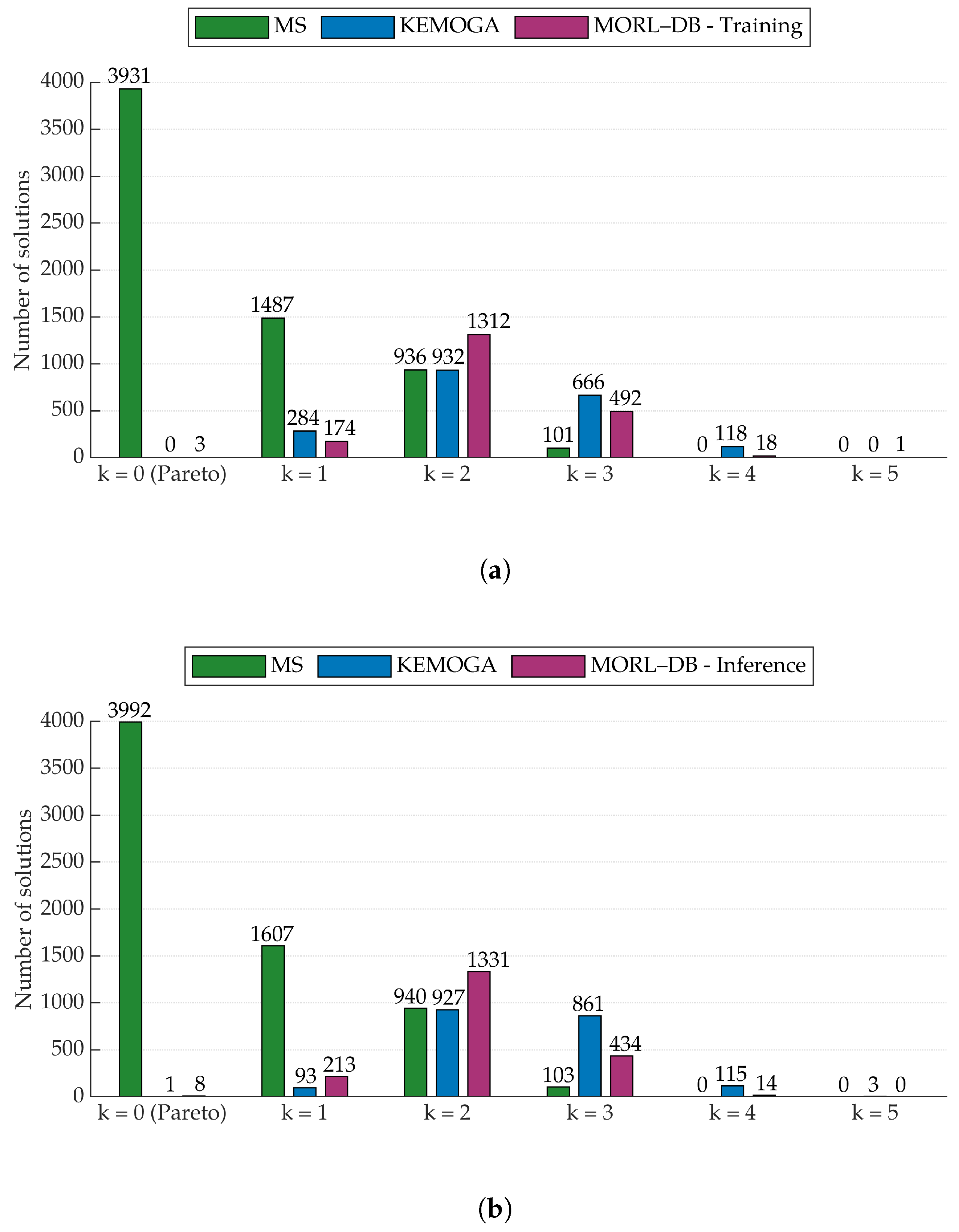
Figure 7 reports the number of optimal design solutions by method and optimality level (see Section 1.1 for the definition of k-optimality). The optimality level of each solution is computed relative to the combined solution sets of all three methods. This enables an objective comparison of method performance in approximating the Pareto front. Most MS solutions have an optimality level $k=0$, indicating good performance for only one objective function. The trend for the MS method optimal design solutions decreases monotonically up to $k=3$, after which no solutions are found. In contrast, KEMOGA and the MORL–DB method produce solutions with a higher optimality level. The MORL–DB method identifies a solution with $k=5$: the remaining Pareto-optimal solutions for any subset of $14-5$ objective functions closer to Utopia than any other solution. The results obtained querying the trained DDPG agent, reported in Figure 7b, are consistent with those produced during training, shown in Figure 7a. This confirms the agent’s capability to identify optimal configurations in an inference phase, i.e., a post-training stage in which the knowledge acquired during learning is exploited [38].

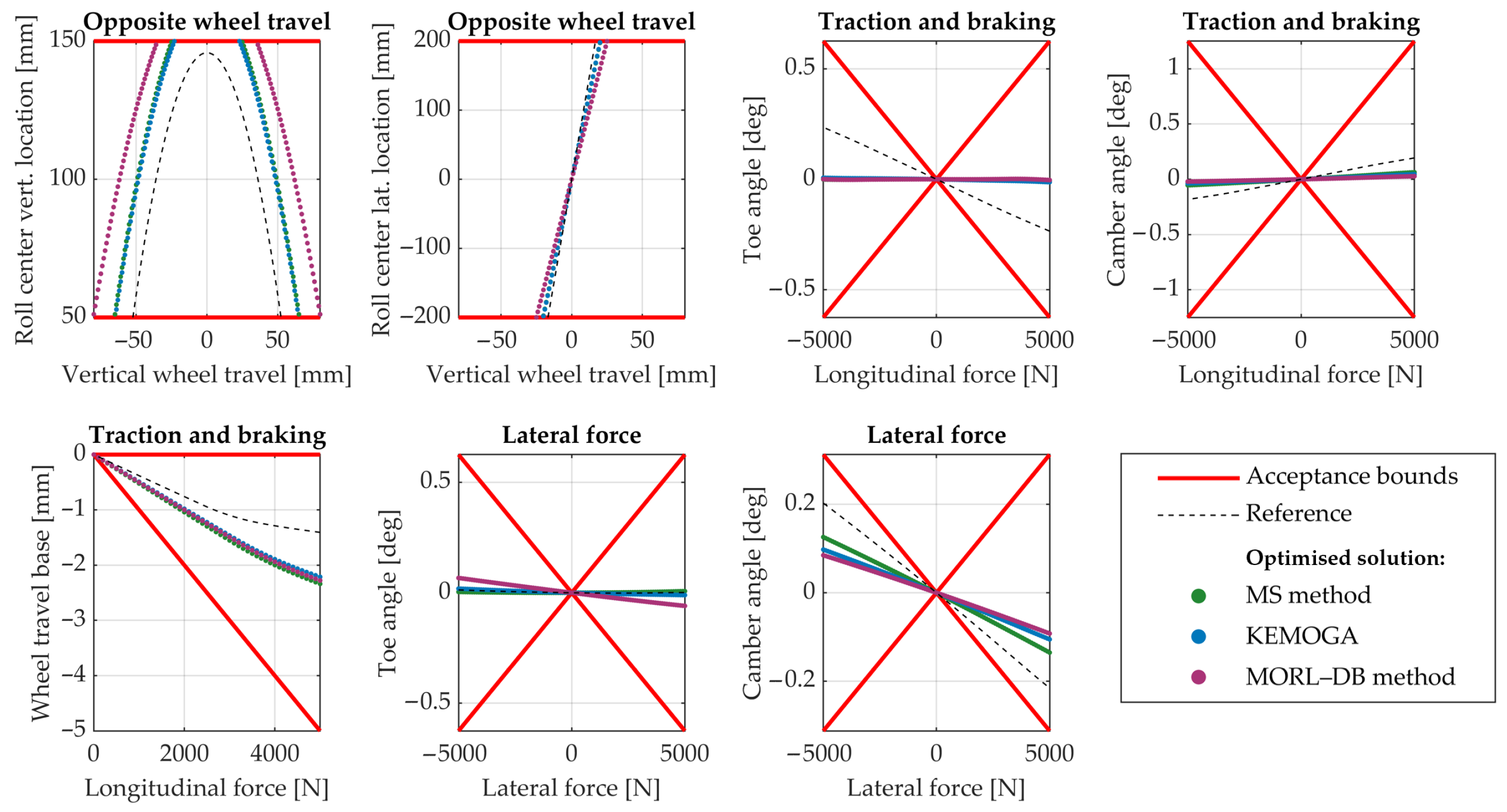
Figure 8 shows the multi-body output curves for the suspension system designed with the MORL–DB method ($k=5$), alongside representative curves from two optimised suspension systems obtained with the MS method ($k=3$) and KEMOGA ($k=4$). In each case, the single solution displayed is selected among those with the highest optimality level achieved by the respective method. All output quantities considered are highly specific to suspension systems [56]. Toe, camber, and caster are three key suspension angles; wheelbase and track are the longitudinal and lateral distances between wheels, respectively. Diving is the attitude of a vehicle to lower the front when braking; anti-dive is the ability to hinder this unwanted motion. Wheel rate is the suspension spring force transmitted to the contact patch per unit vertical wheel displacement. Roll centre denotes the point around which the body of the car rolls in a wheel-fixed frame.

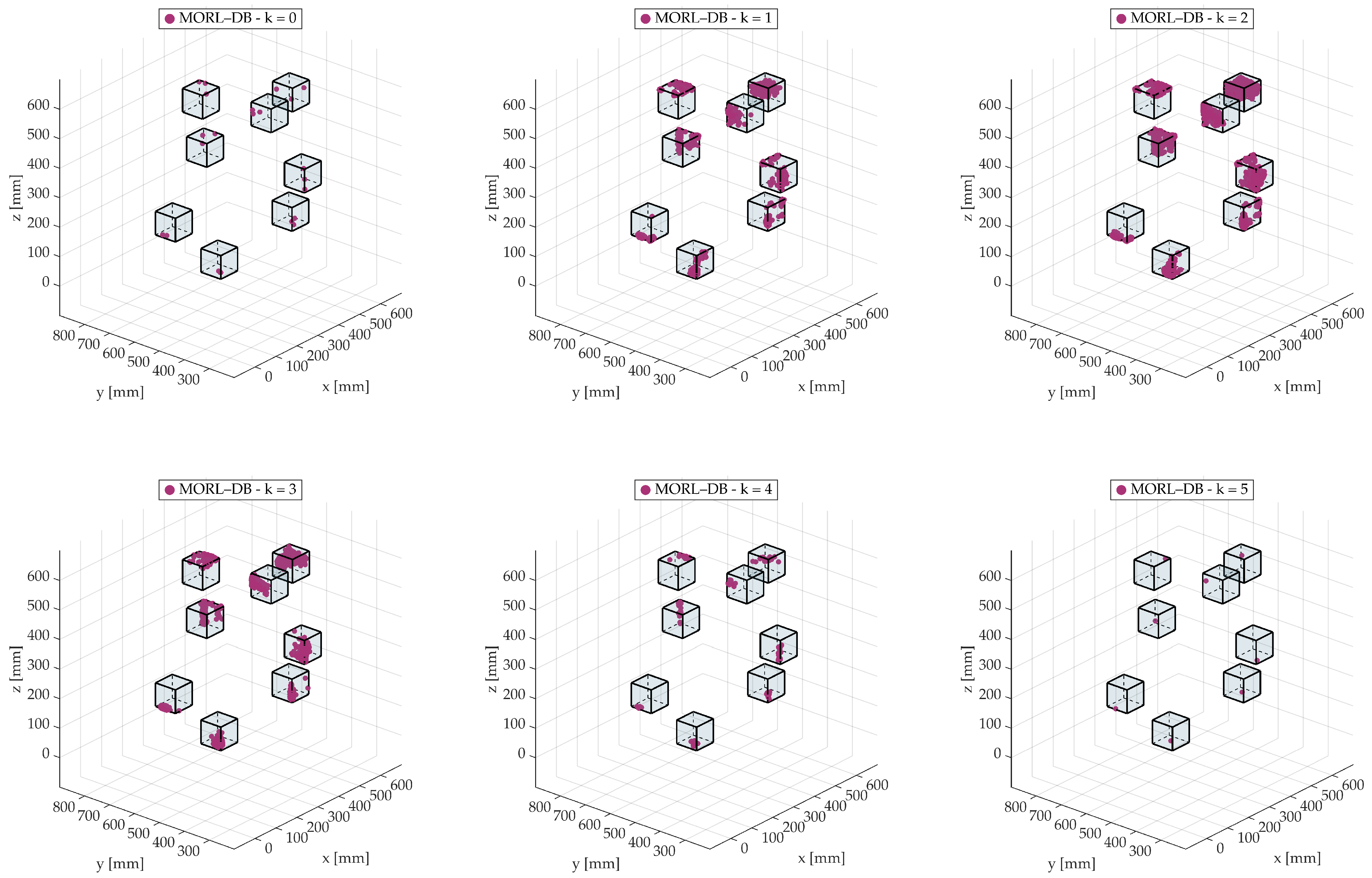
Figure 9 shows the location of the hard points for the optimal design solutions of all three methods inside the design space. Despite unconstrained exploration using KEMOGA and the MORL–DB method inside the design space, all three methods show high consistency, as they find the same optimal regions inside the design space.

5. Discussion

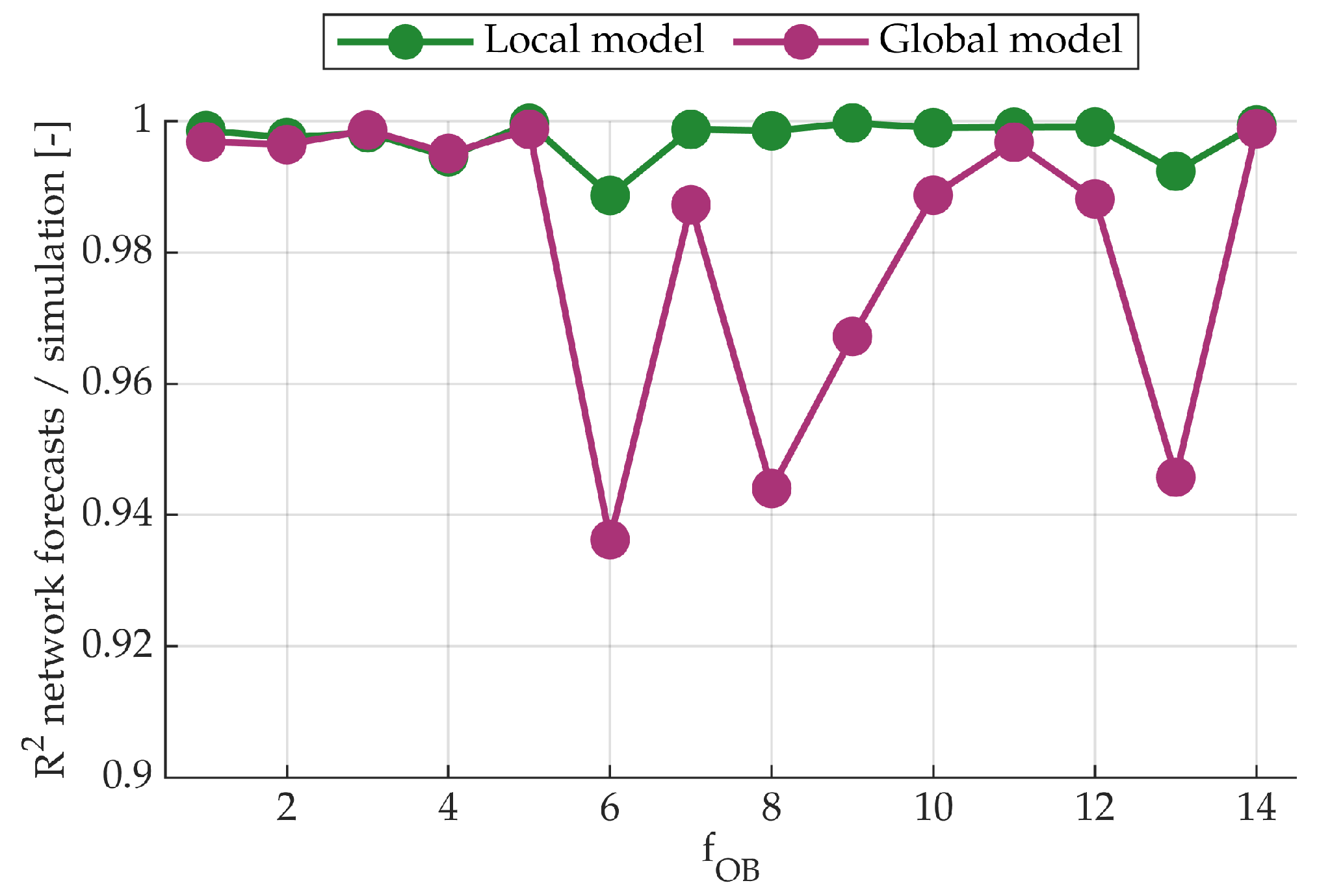
All three methods use surrogate models to approximate the physical model, as each objective function is predicted by a feed-forward neural network rather than computed through a multi-body simulation. The setup parameters for calibrating the feed-forward networks are reported in

Table A1. Parameter settings for the genetic algorithm and neural network used in surrogate model training. The MS method adopts local surrogate models, trained on spherical neighbourhoods (20 mm radius) of a reference suspension configuration. KEMOGA and the MORL–DB method use global surrogate models, trained on data from the full design domain (80 mm-side cube per hard point). Validation metrics are computed considering out-of-sample data. Results for local model are related to the first iteration of the MS method.

Genetic Algorithm Parameters	Local Model	Global Model
Population size	20	20
Maximum number of generations	6	6
Generations without improvement (early stopping)	2	2
Number of training samples	1500	10,000
Design variables for architecture search	Local model	Global model
Neurons in first hidden layer	$[10,22]$	$[10,35]$
Neurons in second hidden layer	$[10,22]$	$[10,35]$
Random seed value	$[0,20]$	$[0,20]$
Neural network configuration
Architecture	Two hidden layers (fully connected)
Input/output normalisation	Min–max scaling to $[-1,1]$
Hidden layer activation function	Logistic sigmoid (logsig)
Output layer activation function	Linear (purelin)
Performance function	Mean squared error (MSE)
Training algorithm	Bayesian regularisation (trainbr)
Data split (train/validation/test)	85%/15%/0%
Splitting method	Random
Training parameters
Maximum number of epochs	1000
Initial learning rate $\mu$	$1\times {10}^{-3}$
Learning rate decrease factor (${\mu }_{dec}$)	$1\times {10}^{-1}$
Learning rate increase factor (${\mu }_{inc}$)	10
Minimum performance gradient	$1\times {10}^{-7}$
Maximum validation failures	6
Validation metrics	Local model	Global model
Lowest $R^2$ on objective functions (forecasts/simulations)	0.989	0.936
Spearman correlation coefficient on k-optimality level (forecasts/simulations)	0.933	0.776

. In the same table, “Genetic algorithm parameters” refers to the algorithm used to optimise the surrogate model, as discussed in phase (A4) of Figure 5. The “local” and “global” attributes specify the extension of the surrogate model approximation: the MORL–DB method and KEMOGA use a global surrogate model; the MS method uses a local one. The local surrogate approximates the physical model only over a sub-portion of the design space, whereas the global surrogate covers the entire design space. Training the global surrogate model can be regarded as an overhead time cost, as this surrogate model substitutes the original multi-body environment for the whole optimisation procedure without requiring retraining. By contrast, the local surrogate model must be retrained at each iteration of the MS method [9], since the portion of the design space being approximated is updated over the iterations of the method. The validation metrics for both surrogate models are reported in Table A1 and in Figure A1.

Setup parameters for MS the method, KEMOGA, and MORL–DB method are reported in

Table A2. Parameter settings for MS method.

Search Space Parameters
Sphere radius	20 mm
Sphere centres	Reference suspension configuration, updated at each iteration
Scaling factors variation	$[0.8,1.2]$, same for all iterations
Search parameters
Iterations performed	5
Configurations tested per iteration	$1\times {10}^6$

,

Table A3. Parameter settings and configuration of the $k\epsilon$ multi-objective genetic algorithm (KEMOGA).

General Settings
Population size	400
Maximum number of generations	40,000
Chromosome encoding	Binary (concatenated genes)
Gene length (bits per variable)	8
Initialisation method	Random
Fitness function	k-optimality
Stopping criterion	Max generations
Selection and elitism
Parent selection method	Roulette wheel (with replacement)
Elitism	Best individuals retained
Duplicate removal	Enabled (per generation)
Crossover and mutation
Crossover method	Single-point
Crossover probability	100%
Number of pairings	Half of the population size
Mutation method	Bit-flip (per gene)
Mutation probability	1%

, and

Table A4. Parameter settings and architectural details for MORL–DB method.

Agent Initialisation and Structure
Number of hidden units per layer	128
Input normalisation	$[0,1]$
Action range	$[-1,1]$
Actor/critic device	GPU
Actor and critic networks
Architecture	Fully connected, 2 hidden layers with 128 units each
Output activation	tanh (actor)/Linear (critic)
Optimisation settings
Optimiser	Adam
Actor/critic learning rate	$5\times {10}^{-4}$
Number of epochs per update	2
Replay buffer and exploration noise
Replay buffer length	10,000
Mini-batch size	256
Warm start steps (commented)	15,000
Initial noise standard deviation	$1\times {10}^{-1}$
Noise standard deviation decay rate	$7.5\times {10}^{-4}$
Learning and update configuration
Discount factor $\gamma$	0.95
Target smoothing factor $\tau$	$1\times {10}^{-2}$
Learning frequency	100
Policy update frequency	2
Number of steps to look ahead	1
Maximum training episodes	400,000

, respectively. Each method was executed until its convergence criterion was satisfied: the MS method converged when the design space became an active constraint, while KEMOGA and the MORL–DB method were stopped after a prescribed number of epochs or episodes, beyond which no sensible improvement in the quality of the solution was observed. The number of configurations generated by the trained DDPG agent was set so that the total configurations processed by the MORL–DB method—considering both training and inference phases—equalled those required by KEMOGA.

Table 5. Summary of computational times and number of design solutions processed for the MS method, KEMOGA, and MORL–DB method. Calculations were performed on a personal computer equipped with an Intel^® Core^TM i7-10750H (2.60–5.00 GHz), 16 GB of RAM, and an NVIDIA Quadro P620 GPU (4 GB).

	MS	KEMOGA	MORL–DB
Computational time
Training set generation (surrogate model)	41 h	54 h 30 m	54 h 30 m
FNN training (surrogate model)	43 h	97 h	97 h
Method-specific computations	35 h	1 h 30 m	3 h 30 m
Optimal design solutions validation	14 h	11 h	11 h
Total	133 h	164 h	166 h
Design solutions processed
By FNN	$5\times {10}^6$	$1.6\times {10}^7$	$4\times {10}^5$
By physical model–training set	7500	10,000	10,000
By physical model–validation set	2500	2000	2000

reports the computational times of the three methods. The MORL–DB inference phase required approximately 1 h 30 m to be performed, reported here for completeness. “Training set generation” refers to the time required to run multi-body simulation in the ADAMS environment in order to generate data for surrogate model training. “FNN training” refers to the time required to train the feed-forward neural networks. This breakdown reflects the different surrogate setups: while the MS method requires repeated training of local surrogate models, the MORL–DB method and KEMOGA rely on a global surrogate model, trained once. In this way, the computational implications of local versus global modelling are explicitly accounted for, ensuring a consistent comparison among the different approaches. “Method-specific computations” denotes the time required by calculations that are specific to the optimisation method. “Optimal design solution validation” corresponds to the time required to validate optimal solutions identified by each method in the ADAMS multi-body environment. Note that all times except method-specific ones arise because of the surrogate model. In principle, all three methods could employ the physical model directly; in this case, most of the surrogate-specific times would be replaced with simulation times.

Table 5 also reports the number of design solutions processed by the feed-forward neural networks. The MORL–DB method processes the fewest solutions, whereas the MS method and KEMOGA process at least one order of magnitude more. The comparison confirms the higher efficiency of the MORL–DB method over the other state-of-the-art methods. The MORL–DB method can handle high-dimensional problems without any scalarisation of the objective functions and requires fewer objective function evaluations. Its performance in settings relying directly on physical models rather than surrogates remains an important direction for further investigation.

Finally, it is worth noting that, at the end of the training, the agent has an in-built knowledge of the state transition, enabling it to move from configurations in the neighbourhood of a reference design toward optimal configuration [38]. In this work, this capability was effectively exploited by querying the trained agent in an inference phase, thereby refining the Pareto-optimal set with additional solutions not identified during training. It is clear that this inference phase cannot be performed with meta-heuristic methods such as KEMOGA, which inherently lacks a learning process.

6. Conclusions

This work presents the general framework of the Multi-Objective Reinforcement Learning–Dominance-Based (MORL–DB) method. It exploits the use of the k-optimality metric to refine the quality of the Pareto-optimal set. The method was applied to the optimal design of a double wishbone suspension system, acting on thirty design variables and optimising fourteen objective functions.

The results of the MORL–DB method are compared to those obtained with the Moving Spheres method and to a multi-objective genetic algorithm with sorting (KEMOGA). Comparative analysis highlights the effectiveness of the MORL–DB method in exploring high-dimensional design spaces. In particular, the MORL–DB method achieved superior k-optimal solutions while requiring only $4\times {10}^5$ objective function evaluations, compared to $5\times {10}^6$ for the MS method and $1.6\times {10}^7$ for KEMOGA. This aspect makes the MORL–DB method particularly suitable for optimisation problems where objective functions evaluations are computationally expensive.

Beyond its computational efficiency, a key novelty of the MORL–DB method lies in the possibility to query the trained RL agent after the learning process, possibly improving the quality of the Pareto-optimal set. This unique capability opens promising directions for future research in the field of optimal design.

References

1. Mastinu, G.; Gobbi, M.; Miano, C. Optimal Design of Complex Mechanical Systems: With Applications to Vehicle Engineering; Springer Science & Business Media: Berlin/Heidelberg, Germany; New York, NY, USA, 2007. [Google Scholar]
2. Sacks, J.; Welch, W.J.; Mitchell, T.J.; Wynn, H.P. Design and Analysis of Computer Experiments. Stat. Sci. 1989, 4, 409–423. [Google Scholar] [CrossRef]
3. Forrester, A.I.J.; Sóbester, A.; Keane, A.J. Engineering Design via Surrogate Modelling; Wiley: Hoboken, NJ, USA, 2008. [Google Scholar] [CrossRef]
4. Giunta, A.; Watson, L. A comparison of approximation modeling techniques—Polynomial versus interpolating models. In Proceedings of the 7th AIAA/USAF/NASA/ISSMO Symposium on Multidisciplinary Analysis and Optimization. American Institute of Aeronautics and Astronautics, St. Louis, MO, USA, 2–4 September 1998. [Google Scholar] [CrossRef]
5. Yıldız, B.S.; Yıldız, A.R.; İsa Albak, E.; Abderazek, H.; Sait, S.M.; Bureerat, S. Butterfly optimization algorithm for optimum shape design of automobile suspension components. Mater. Test. 2020, 62, 365–370. [Google Scholar] [CrossRef]
6. Barthelemy, J.F.M.; Haftka, R.T. Approximation concepts for optimum structural design—A review. Struct. Optim. 1993, 5, 129–144. [Google Scholar] [CrossRef]
7. Gobbi, M.; Mastinu, G.; Doniselli, C.; Guglielmetto, L.; Pisino, E. Optimal & Robust Design of a Road Vehicle Suspension System. Veh. Syst. Dyn. 1999, 33, 3–22. [Google Scholar] [CrossRef]
8. Gobbi, M.; Mastinu, G.; Doniselli, C. Optimising a Car Chassis. Veh. Syst. Dyn. 1999, 32, 149–170. [Google Scholar] [CrossRef]
9. De Santanna, L.; Gobbi, M.; Malacrida, R.; Mastinu, G. Multi-objective optimisation of complex mechanisms using Moving Spheres: An application to suspension elasto-kinematics. Adv. Eng. Softw. 2025, 208, 103974. [Google Scholar] [CrossRef]
10. Barri, D.; Soresini, F.; Gobbi, M.; Gerlando, A.d.; Mastinu, G. Optimal Design of Traction Electric Motors by a New Adaptive Pareto Algorithm. IEEE Trans. Veh. Technol. 2025, 74, 8890–8906. [Google Scholar] [CrossRef]
11. Holland, J.H. Adaptation in Natural and Artificial Systems; The MIT Press: Cambridge, MA, USA, 1992. [Google Scholar] [CrossRef]
12. Benedetti, A.; Farina, M.; Gobbi, M. Evolutionary multiobjective industrial design: The case of a racing car tire-suspension system. IEEE Trans. Evol. Comput. 2006, 10, 230–244. [Google Scholar] [CrossRef]
13. Abualigah, L.; Elaziz, M.A.; Khasawneh, A.M.; Alshinwan, M.; Ibrahim, R.A.; Al-qaness, M.A.A.; Mirjalili, S.; Sumari, P.; Gandomi, A.H. Meta-heuristic optimization algorithms for solving real-world mechanical engineering design problems: A comprehensive survey, applications, comparative analysis, and results. Neural Comput. Appl. 2022, 34, 4081–4110. [Google Scholar] [CrossRef]
14. Glover, F. Future paths for integer programming and links to artificial intelligence. Comput. Oper. Res. 1986, 13, 533–549. [Google Scholar] [CrossRef]
15. Kennedy, J.; Eberhart, R. Particle swarm optimization. In Proceedings of the IEEE International Conference on Neural Networks—Conference Proceedings, Perth, Australia, 27 November–1 December 1995; Volume 4, pp. 1942–1948. [Google Scholar]
16. Dorigo, M.; Maniezzo, V.; Colorni, A. Ant system: Optimization by a colony of cooperating agents. IEEE Trans. Syst. Man, Cybern. Part (Cybern.) 1996, 26, 29–41. [Google Scholar] [CrossRef]
17. Hedar, A.R.; Abdel-Hakim, A.E.; Deabes, W.; Alotaibi, Y.; Bouazza, K.E. Deep Memory Search: A Metaheuristic Approach for Optimizing Heuristic Search. arXiv 2024, arXiv:2410.17042. [Google Scholar] [CrossRef]
18. Tomar, V.; Bansal, M.; Singh, P. Metaheuristic Algorithms for Optimization: A Brief Review. Eng. Proc. 2024, 59, 238. [Google Scholar] [CrossRef]
19. Benaissa, B.; Kobayashi, M.; Ali, M.A.; Khatir, T.; Elmeliani, M.E.A.E. Metaheuristic optimization algorithms: An overview. Hcmcou J. Sci. Adv. Comput. Struct. 2024, 14, 33–61. [Google Scholar] [CrossRef]
20. De Santanna, L.; Guidotti, G.; Mastinu, G.; Gobbi, M. Multi-objective optimal design based on Reinforcement Learning. J. Mech. Des. 2025, 147, 101703. [Google Scholar] [CrossRef]
21. Wang, Z.; Zeng, T.; Chu, X.; Xue, D. Multi-objective deep reinforcement learning for optimal design of wind turbine blade. Renew. Energy 2023, 203, 854–869. [Google Scholar] [CrossRef]
22. Zitzler, E.; Deb, K.; Thiele, L. Comparison of Multiobjective Evolutionary Algorithms: Empirical Results. Evol. Comput. 2000, 8, 173–195. [Google Scholar] [CrossRef]
23. Srinivas, N.; Deb, K. Muiltiobjective Optimization Using Nondominated Sorting in Genetic Algorithms. Evol. Comput. 1994, 2, 221–248. [Google Scholar] [CrossRef]
24. Yonekura, K.; Yamada, R.; Ogawa, S.; Suzuki, K. Hypervolume-Based Multi-Objective Optimization Method Applying Deep Reinforcement Learning to the Optimization of Turbine Blade Shape. AI 2024, 5, 1731–1742. [Google Scholar] [CrossRef]
25. Guerreiro, A.P.; Fonseca, C.M.; Paquete, L. The Hypervolume Indicator: Computational Problems and Algorithms. ACM Comput. Surv. 2022, 54, 1–42. [Google Scholar] [CrossRef]
26. Yang, F.; Huang, H.; Shi, W.; Ma, Y.; Feng, Y.; Cheng, G.; Liu, Z. PMDRL: Pareto-front-based multi-objective deep reinforcement learning. J. Ambient. Intell. Humaniz. Comput. 2023, 14, 12663–12672. [Google Scholar] [CrossRef]
27. Mnih, V.; Kavukcuoglu, K.; Silver, D.; Rusu, A.A.; Veness, J.; Bellemare, M.G.; Graves, A.; Riedmiller, M.; Fidjeland, A.K.; Ostrovski, G.; et al. Human-level control through deep reinforcement learning. Nature 2015, 518, 529–533. [Google Scholar] [CrossRef]
28. Barto, A.G.; Sutton, R.S.; Anderson, C.W. Neuronlike adaptive elements that can solve difficult learning control problems. IEEE Trans. Syst. Man Cybern. 1983, SMC-13, 834–846. [Google Scholar] [CrossRef]
29. Seurin, P.; Shirvan, K. Multi-objective reinforcement learning-based approach for pressurized water reactor optimization. Ann. Nucl. Energy 2024, 205, 110582. [Google Scholar] [CrossRef]
30. Deb, K.; Thiele, L.; Laumanns, M.; Zitzler, E. Scalable multi-objective optimization test problems. In Proceedings of the 2002 Congress on Evolutionary Computation, Honolulu, HI, USA, 12–17 May 2002; IEEE: Piscataway, NJ, USA, 2002; pp. 825–830. [Google Scholar] [CrossRef]
31. Jain, H.; Deb, K. An Evolutionary Many-Objective Optimization Algorithm Using Reference-Point Based Nondominated Sorting Approach, Part II: Handling Constraints and Extending to an Adaptive Approach. IEEE Trans. Evol. Comput. 2014, 18, 602–622. [Google Scholar] [CrossRef]
32. Deb, K.; Pratap, A.; Meyarivan, T. Constrained Test Problems for Multi-objective Evolutionary Optimization. In Proceedings of the Evolutionary Multi-Criterion Optimization, Zurich, Switzerland, 7–9 March 2001; Zitzler, E., Thiele, L., Deb, K., Coello Coello, C.A., Corne, D., Eds.; Springer: Berlin/Heidelberg, Germany, 2001; pp. 284–298. [Google Scholar] [CrossRef]
33. Deb, K.; Pratap, A.; Agarwal, S.; Meyarivan, T. A fast and elitist multiobjective genetic algorithm: NSGA-II. IEEE Trans. Evol. Comput. 2002, 6, 182–197. [Google Scholar] [CrossRef]
34. Deb, K.; Jain, H. An Evolutionary Many-Objective Optimization Algorithm Using Reference-Point-Based Nondominated Sorting Approach, Part I: Solving Problems With Box Constraints. IEEE Trans. Evol. Comput. 2014, 18, 577–601. [Google Scholar] [CrossRef]
35. Suppapitnarm, A.; Seffen, K.A.; Parks, G.T.; Clarkson, P.J. Simulated Annealing algorithm for multiobjective optimization. Eng. Optim. 2000, 33, 59–85. [Google Scholar] [CrossRef]
36. Ebrie, A.S.; Kim, Y.J. Reinforcement Learning-Based Multi-Objective Optimization for Generation Scheduling in Power Systems. Systems 2024, 12, 106. [Google Scholar] [CrossRef]
37. Kupwiwat, C.-t.; Hayashi, K.; Ohsaki, M. Multi-objective optimization of truss structure using multi-agent reinforcement learning and graph representation. Eng. Appl. Artif. Intell. 2024, 129, 107594. [Google Scholar] [CrossRef]
38. NS, K.S.; Li, P. Pareto Optimization of Analog Circuits Using Reinforcement Learning. ACM Trans. Des. Autom. Electron. Syst. 2024, 29, 1–14. [Google Scholar] [CrossRef]
39. Yang, R.; Sun, X.; Narasimhan, K. A generalized algorithm for multi-objective reinforcement learning and policy adaptation. In Proceedings of the 33rd International Conference on Neural Information Processing Systems, Red Hook, NY, USA, 8–14 December 2019; pp. 1311–1322. [Google Scholar]
40. Sato, T.; Watanabe, K. A Data-Driven Automatic Design of Induction Motors Based on Tree Search and Reinforcement Learning Considering Multiple Objectives. IEEE Trans. Magn. 2024, 60, 1–4. [Google Scholar] [CrossRef]
41. Deb, K.; Saxena, D. On Finding Pareto-Optimal Solutions Through Dimensionality Reduction for Cretain Large-Dimensional Multi-Objective Optimization Problems; Technical Report KanGAL Report No. 2005011; Department of Mechanical Engineering, IIT: Kanpur, India, 2005. [Google Scholar]
42. Kukkonen, S.; Lampinen, J. Ranking-Dominance and Many-Objective Optimization. In Proceedings of the 2007 IEEE Congress on Evolutionary Computation, Singapore, 25–28 September 2007; IEEE: Piscataway, NJ, USA, 2007; pp. 3983–3990. [Google Scholar] [CrossRef]
43. Levi, F.; Gobbi, M.; Farina, M.; Mastinu, G. Multi-Objective Design and Selection of One Single Optimal Solution. In Proceedings of the Design Engineering, ASMEDC, Anaheim, CA, USA, 13–19 November 2004; pp. 841–848. [Google Scholar]
44. Gobbi, M. A k, k-ε optimality selection based multi objective genetic algorithm with applications to vehicle engineering. Optim. Eng. 2013, 14, 345–360. [Google Scholar] [CrossRef]
45. De Santanna, L.; Gobbi, M.; Malacrida, R.; Mastinu, G. Optimal Multi-Objective Elasto-Kinematic Design of a Suspension System by Means of Artificial Intelligence. In Proceedings of the 26th International Conference on Advanced Vehicle Technologies (AVT), ASME 2025 International Design Engineering Technical Conferences & Computers and Information in Engineering Conference (IDETC/CIE), Anaheim, CA, USA, 17–20 August 2025. Paper No. 169160, Session AVT-02/07. [Google Scholar]
46. Hollenstein, J.; Auddy, S.; Saveriano, M.; Renaudo, E.; Piater, J. Action Noise in Off-Policy Deep Reinforcement Learning: Impact on Exploration and Performance. arXiv 2023, arXiv:2206.03787. [Google Scholar] [CrossRef]
47. Zhu, S.; He, Y. A Design Synthesis Method for Robust Controllers of Active Vehicle Suspensions. Designs 2022, 6, 14. [Google Scholar] [CrossRef]
48. Cheli, F.; Diana, G. Advanced Dynamics of Mechanical Systems; Springer International Publishing: Berlin/Heidelberg, Germany, 2015. [Google Scholar] [CrossRef]
49. Shabana, A.A. Computational Dynamics; Wiley: Hoboken, NJ, USA, 2010. [Google Scholar] [CrossRef]
50. Țoțu, V.; Alexandru, C. Multi-Criteria Optimization of an Innovative Suspension System for Race Cars. Appl. Sci. 2021, 11, 4167. [Google Scholar] [CrossRef]
51. Avi, A.G.; Carboni, A.P.; Costa, P.H.S. Multi-objective optimization of the kinematic behaviour in double wishbone suspension systems using genetic algorithm. In Proceedings of the 2020 SAE Brasil Congress & Exhibition, Sao Paulo, Brasil, 1 December 2020. SAE Technical Paper 2020-36-0154. [Google Scholar] [CrossRef]
52. Bagheri, M.R.; Mosayebi, M.; Mahdian, A.; Keshavarzi, A. Multi-objective optimization of double wishbone suspension of a kinestatic vehicle model for handling and stability improvement. Struct. Eng. Mech. 2018, 68, 633–638. [Google Scholar] [CrossRef]
53. Olschewski, J.; Fang, X. Elastokinematic design and optimization of the multi-link torsion axle—A novel rear axle concept for BEVs. Mech. Based Des. Struct. Mach. 2025, 53, 301–332. [Google Scholar] [CrossRef]
54. Magri, P.; Gadola, M.; Chindamo, D.; Sandrini, G. A Comprehensive Method for Computing Non-Linear Elastokinematic Properties of Passenger Car Suspension Systems: Double Wishbone Case Study. J. Comput. Nonlinear Dyn. 2024, 19, 101006. [Google Scholar] [CrossRef]
55. Arshad, M.W.; Lodi, S.; Liu, D.Q. Multi-Objective Optimization of Independent Automotive Suspension by AI and Quantum Approaches: A Systematic Review. Machines 2025, 13, 204. [Google Scholar] [CrossRef]
56. Guiggiani, M. The Science of Vehicle Dynamics; Springer: Berlin/Heidelberg, Germany, 2023. [Google Scholar] [CrossRef]
Figure 1. Trend of the ratio between the size of the optimal design solution set and the whole design solution set with a different number of objective functions. (a): Pareto-optimal set; (b): best k-optimality level set. Each data point is computed as the mean over 1000 independently generated problems, each represented by a matrix of 10,000 randomly sampled solutions. Circles indicate the average fraction of optimal solutions, while vertical segments represent the corresponding standard deviation.
Designs 09 00108 g001
Figure 2. Reinforcement Learning framework.
Designs 09 00108 g002
Figure 3. Flowchart of the DDPG algorithm. In design optimisation, the system state depends on design variables rather than on time, as is common in typical Reinforcement Learning applications.
Designs 09 00108 g003
Figure 4. Objective function evaluation procedure based on multi-body simulation output curves. (a): Generic simulation output, acceptance bounds, and target. The horizontal axis x is the independent variable of the simulation. (b): Trend of ν , as a function of the distance between the multi-body output curve and the target. Circles in (a), representing generic multi-body simulation outputs f ( x i ) , are mapped into ν values in (b). The objective function value associated to the given simulation output is the arithmetic mean of all ν ( x i ) .
Designs 09 00108 g004
Figure 5. Workflow of Multi-Objective Reinforcement Learning–Dominance-Based (MORL–DB) method. The proposed implementation employs a surrogate model to approximate the behaviour of the system to be optimised.
Designs 09 00108 g005
Figure 6. Multi-body model of the double wishbone suspension used in the test case. Circles highlight hard points included in the optimisation. Scaling factors of the bushings on hard points 1 and 3 are also included in the optimisation.
Designs 09 00108 g006
Figure 7. Optimal design solutions from the three methods considered, grouped by k-optimality; 0-optimality corresponds to Pareto optimality. (a): MORL–DB solutions are selected among the ones obtained during agent training. (b): MORL–DB solutions are determined querying the trained agent.
Designs 09 00108 g007
Figure 8. Multi-body output curves (see Table 4) for the suspension system designed with the MORL–DB method, and for the suspensions designed through the MS method and KEMOGA (one configuration selected among the ones with the best k-optimality level). The behaviour of the reference suspension is also reported for comparison. The acceptance bounds are shown in red.
Designs 09 00108 g008aDesigns 09 00108 g008b
Figure 9. Locations of the hard points of all optimal solutions obtained through the MORL–DB method inside the design space, grouped by their k-optimality level.
Designs 09 00108 g009