Comparative Analysis of Various Hyperelastic Models and Element Types for Finite Element Analysis

Abstract

This study aims to evaluate the precision of nine distinct hyperelastic models using experimental data sourced from the existing literature. These models rely on parameters obtained through curve-fitting functions. The complexity in finite element models of elastomers arises due to their nonlinear, incompressible behaviour. To achieve accurate representations, it is imperative to employ sophisticated hyperelastic models and appropriate element types and formulations. Prior published work has primarily focused on the comparison between the fitting models and the experimental data. Instead, in this study, the results obtained from finite element analysis are compared against the original data to assess the impact of element formulation, strain range, and mesh type on the ability to accurately predict the response of elastomers over a wide range of strain values. This comparison confirms that the element formulation and strain range can significantly influence result accuracy, yielding different responses in various strain ranges also because of the limitation with the curve fitting tools.

1. Introduction

Elastomers can be classified based on various criteria, including composition and vulcanization [1]. In contrast to isotropic metals, isotropic rubber demonstrates pronounced nonlinearity in its elastic behaviour when subjected to stress and strain [2]. Rubber features an extensive elastic range, often surpassing metals by up to 500%, and it also displays high internal damping when subjected to dynamic loads. These characteristics make it particularly well suited for applications such as rubber mounts.

Owing to the extensive elastic range of rubber, the conventional small strain theory is insufficient for describing its behaviour [3]. Instead, the material’s response is characterized by its strain energy density function, often referred to as the Helmholtz free energy [1], which also considers temperature effects. To achieve a complete understanding of the significant deformations in rubber, continuum mechanics is employed to describe the motion of each material point [1,2]. Various constitutive equations have been developed to mathematically capture material behaviour, considering both stress–strain relationships and temperature effects. Cauchy stress constitutive equations (Equation (1)) [1] establish a connection between Cauchy stress (σ) and strain energy density (W(F)), factoring in deformation gradient (F) and volumetric deformation (J).

$$\sigma \left(F\right)=\frac{1}{J}\frac{\partial W(F)}{\partial F}{F}^T$$

(1)

While no material can be considered fully incompressible, elastomers are often treated as nearly incompressible materials with a Poisson’s ratio assumed to be approximately 0.5. In the case of incompressible elastomers, when the volumetric deformation (J) equals one [4], the Cauchy stress constitutive equation can be simplified from Equations (1) and (2) [1]. Here, p represents the pressure applied to the elastomer, b is the left Cauchy stress tensor, I₁ and I₂ denote the first and second Cauchy stress invariants, and I represent the identity matrix.

$$\sigma =2\left(\frac{\partial W}{\partial I_1}+I_1\frac{\partial W}{\partial I_2}\right)b-2\frac{\partial W}{\partial I_2}{b}^2+pI$$

(2)

Various strain energy functions (SEFs) (W(F)) are employed in constitutive equations, each corresponding to distinct stress–strain responses [2].

Broadly, hyperelastic models fall into three categories: phenomenological, micro-mechanical, and hybrid, a combination of the prior two [2,5]. Phenomenological models derive from ideal elastomer properties within continuum mechanics [2,5], while micro-mechanical models stem from the microstructural response at the polymeric chain level [2,5]. Hybrid models integrate both approaches [5] and demand greater computational power compared to phenomenological models. Yet, recent studies suggest they can relate macroscopic mechanical behaviour to physical or chemical structural changes [5].

Phenomenological models encompass neo-Hookean, two-term reduced polynomial, Mooney–Rivlin, three-term Ogden, two-term polynomial, Yeoh, and Marlow [5], while Arruda–Boyce is micro-mechanical, and van der Waals is a hybrid model [5].

These models share a common feature as they facilitate nonlinear finite element analysis (FEA) of various elastomer components like response of oil palm shell-reinforced rubber (ROPS) composites with different oil palm shell (OPS) contents and shapes [6], automotive weatherstripping [7], and antivibration systems [8].

Accurate numerical simulations of rubber-like materials (RLMs) necessitate reliable hyperelastic models. Accuracy of a hyperelastic model is defined by how closely the predicted stress matches stresses derived from mechanical tests [1]. Thus, many studies have compared different hyperelastic models’ accuracy under large strain deformation. Typically, accuracy comparisons rely on stress–strain curves derived from strain energy functions [9,10], wherein stress–strain curves from three mechanical tests are compared with model predictions. Recent studies [10,11,12,13,14] have compared the accuracy of a large number of hyperelastic models, deriving their own strain energy functions. Studies have also explored how fitting algorithm formulations affect the generation of material parameters and prediction accuracy [12,13,14]. Studies have examined accuracy under biaxial deformation [15], comparing model-predicted stress with mechanical test results. An extensive study on the Odgen model [16] compared the accuracy of the original Odgen model with other variations.

A recent study conducted a comprehensive comparison of 85 distinct hyperelastic models, encompassing models ranging from the early 1990s to more recent ones [10]. The primary focus of this investigation was centred on hyperelastic responses under static or quasi-static loads, neglecting stress stiffening, the Payne effect, and similar phenomena [10]. Additionally, the study selected 10 models to undergo numerical simulations for uniaxial tensile testing with strains below 1.5, employing Abaqus CAE for these simulations. The material was treated as incompressible, and the chosen element was C8D8RH, a linear hexagonal hybrid element with reduced integration without providing a detailed description of the zero-energy modes.

Historically, the prior literature has commonly favoured linear hexagonal elements for numerical simulations involving rubber-like materials [6,8,10]. In cases where components exhibit intricate curvature, automated meshing tools may also come into play; however, these tools are typically limited to tetrahedral elements [17].

This study presents an investigation into the accuracy of different hyperelastic models and element formulations under monotonically quasi-static loading conditions. The stress–strain response is obtained from a simulation analysing the force displacement data to capture the overall response of the simulated specimens. Results from simulations have been compared against the experimental data used for the curve-fitting of the hyperelastic material model. The following hyperelastic models are explored in this study: two-term reduced polynomial, Arruda–Boyce, Marlow, Mooney–Rivlin, neo-Hookean, three-term Ogden, two-term polynomial, van der Waals, and Yeoh. Detailed mathematical formulations are provided in the following section.

2. Hyperelastic Material Models

To comprehensively characterize the intricate behaviour of elastomers, various methodologies are available. These approaches result in different formulations of strain energy functions or models. Hyperelastic models exhibit variations in terms of their complexity and the number of material parameters involved. Typically, more intricate models involve a greater number of material parameters and more complex equations. Some models prioritize user-friendliness, but to achieve this, the strain energy function may undergo simplification, which might involve omitting the second deviatoric stress invariant and utilizing fewer material parameters. These divergences can yield fundamentally distinct stress–strain predictions. As such, this study places significant importance on evaluating the accuracy of each hyperelastic model, as these models directly impact the precision of numerical simulation results.

In a three-dimensional space, where the principal stresses align with the main axes [18], a vector can represent the stress state.

Figure 1 shows a particular stress state of a point “$P$”. The hydrostatic axis (z) is the axis in which the three principal stresses are equal σ₁ = σ₂ = σ₃. The plane containing $P$ and perpendicular to the hydrostatic axis is called the deviatoric plane.

$P$ can also be represented geometrically in terms of the three invariants of the stress tensor. Assuming that the three principal stresses have the following order, σ₁ ≥ σ₂ ≥ σ₃, the hydrostatic stress or the first stress invariant I₁ is the distance from the origin to the deviatoric plane containing the point P ($\left|O{O}^{\prime }\right|$) with the three stress invariants $I_1$, $I_2$, and $I_3$ as follows:

$$\left|O{O}^{\prime }\right|=\sqrt{3}{\sigma }_m=\frac{I_1}{\sqrt{3}}$$

(3)

$$I_1={\sigma }_1+{\sigma }_2+{\sigma }_3={{\lambda }_1}^2+{{\lambda }_2}^2+{{\lambda }_3}^2=3{\sigma }_m$$

(4)

$$I_2={\sigma }_{11}{\sigma }_{22}+{\sigma }_{22}{\sigma }_{33}+{\sigma }_{33}{\sigma }_{11}-{\sigma }_{12}^2-{\sigma }_{13}^2-{\sigma }_{23}^2={{\lambda }_1}^2{{\lambda }_2}^2+{{\lambda }_2}^2{{\lambda }_3}^2+{{\lambda }_1}^2{{\lambda }_3}^2$$

(5)

$$I_3={\sigma }_{11}{\sigma }_{22}{\sigma }_{33}-{\sigma }_{11}{\sigma }_{23}^2-{\sigma }_{22}{\sigma }_{13}^2-{\sigma }_{33}{\sigma }_{12}^2+2{\sigma }_{12}{\sigma }_{13}{\sigma }_{23}={{\lambda }_1}^2{{\lambda }_2}^2{{\lambda }_3}^2$$

(6)

The stress invariants can be expressed using stretch ratios (λ₁, λ₂, λ₃). This format for stretch ratios has been widely adopted in previous studies and research, simplifying the discussion about hyperelastic models [1,9].

Furthermore, tensors can be decomposed into two components: a deviatoric part and a volumetric part. Most of the hyperelastic models are based on the decomposition of Cauchy stress invariants. The process of decomposition is outlined in Equation (7) [1], where ‘A’ can represent the first, second, or third Cauchy stress invariant. The deviatoric and volumetric parts are represented by Equations (8) and (9) [1].

$$A=dev\left[A\right]+vol\left[A\right]$$

(7)

$$dev[A]=A-\frac{1}{3}tr\left[A\right]I$$

(8)

$$vol[A]=\frac{1}{3}tr\left[A\right]I$$

(9)

The accuracy of stress–strain responses is assessed in both material element predictions and numerical simulations. Hyperelastic models can predict large strain deformation accurately under static or quasi-static load [1], without the need for more complex viscoelastic formulations such as rheological models. For this reason, this work only focuses on large strain deformation with viscoelasticity and stress softening related to the Mullin effect not considered [1]. Strain energy functions for each hyperelastic model are reported in brief in the following subsections.

2.1. Neo-Hookean

Considering the stress tensor and the expression of the invariants of the stress tensor, the neo-Hookean model is the simplest hyperelastic model amongst those considered in this study, since it only depends on the first deviatoric invariant $\overline{I_1}$. The material parameters for neo-Hookean are $C_{10}$ and $D_1$, where $C_{10}$ depends on shear modulus $\mu$, and $D_1$ depends on bulk modulus κ. J_el is the elastic volume ratio [1].

$$W=C_{10}\left(\overline{I_1}-3\right)+\frac{1}{D_1}(J_{el}-1{)}^2$$

(10)

2.2. Mooney–Rivlin

The Mooney–Rivlin model is based on the neo-Hookean model with an additional term featuring the second deviatoric invariant $\overline{I_2}$. The material parameters for Mooney–Rivlin are $C_{10}$, $C_{01}$, and $D_1$, where $C_{10}$ and $C_{01}$ depend on shear modulus $\mu$, whilst $D_1$ depends on bulk modulus κ [1].

$$W=C_{10}\left(\overline{I_1}-3\right)+C_{01}(\overline{I_2}-3)+\frac{1}{D_1}(J_{el}-1{)}^2$$

(11)

2.3. Two-Term Reduced Polynomial

The two-term reduced polynomial form is also based on neo-Hookean, with an added term using the first deviatoric invariant $\overline{I_1}$. The material parameters for two-term reduced polynomial are $C_{10}$, $C_{20}$, $D_1$, and $D_2$ where $C_{10}$ and $C_{20}$ depend on shear modulus $\mu$, whilst $D_1$ and $D_2$ depend on bulk modulus κ [1].

$$W=C_{10}\left(\overline{I_1}-3\right)+{C_{20}(\overline{I_1}+3)}^2+\sum _{i=1}^2\frac{1}{D_i}(J_{el}-1{)}^{2i}$$

(12)

2.4. Two-Term Polynomial

The two-term polynomial form includes both the first and second deviatoric invariants. As the two-term polynomial form is more complex than neo-Hookean, it needs more material parameters. The material parameters are $C_{10}$, $C_{01}$, $C_{11}$, $C_{20}$, $C_{02}$, $D_1$, and $D_2$, where $C_{10}$, $C_{01}$, $C_{11}$, $C_{20}$, and $C_{02}$ depend on shear modulus $\mu$, and $D_1$ and $D_2$ depend on the bulk modulus κ [1].

$$W=\sum _{i+j=1}^2{C_{ij}(\overline{I_1}-3)}^i{(\overline{I_2}-3)}^j+\sum _{i=1}^2\frac{1}{D_i}(J_{el}-1{)}^{2i}$$

(13)

2.5. Yeoh

The Yeoh form is very similar to the two-term reduced polynomial form, as it can also be considered as the three-term reduced polynomial form. The material parameters for the Yeoh form are: $C_{10}$, $C_{20}$, $C_{30}$, $D_1$, $D_2$, and $D_3$, where $C_{10}$, $C_{20}$, and $C_{30}$ depend on the shear modulus $\mu$, and $D_1$, $D_2$, and $D_3$ depend on the bulk modulus κ [1].

$$W=C_{10}\left(\overline{I_1}-3\right)+{C_{20}(\overline{I_1}+3)}^2+{C_{30}(\overline{I_1}+3)}^3+\frac{1}{D_1}(J_{el}-1{)}^2+\frac{1}{D_2}(J_{el}-1{)}^4+\frac{1}{D_3}(J_{el}-1{)}^6$$

(14)

2.6. Arruda–Boyce

Arruda–Boyce form is also known as the eight-chain form, as this model is based on how elastomer’s microstructure deforms. Arruda–Boyce only depends on the first deviatoric invariant. Material parameters for Arruda–Boyce are: $\mu$, ${\lambda }_m$, and $D$; notice that $C_1$ to $C_5$ are not material parameters but just constants. $\mu$ is the shear modulus, and $D$ is a parameter related to bulk modulus κ. Parameter ${\lambda }_m$ is the maximum stretch of the molecule chain [1].

$$W=\mu \sum _{i=5}^5\frac{C_i}{{{\lambda }_m}^{2i-2}}\left({\overline{I_1}}^i-3^i\right)+\frac{1}{D}(\frac{{J_{el}}^2-1}{2}-\ln J_{el})$$

(15)

2.7. Three-Term Ogden

The three-term Ogden form is dependent on the first, second, and third principle stretches instead of deviatoric invariants. The model parameters are: ${\alpha }_1$, ${\alpha }_2$, ${\alpha }_3$, ${\mu }_1$, ${\mu }_2$, ${\mu }_3$, $D_1$, $D_2$, and $D_{3 }$, where ${\mu }_1$ to ${\mu }_{13}$ and ${\alpha }_1$ to ${\alpha }_3$ are parameters related to shear modulus $\mu$, and $D_1$ to $D_3$ are related to bulk modulus κ [1].

$$W=\sum _{i=1}^3\frac{2{\mu }_i}{{{\alpha }_i}^2}\left({\overline{{\lambda }_1}}^{{\alpha }_i}+{\overline{{\lambda }_2}}^{{\alpha }_i}+{\overline{{\lambda }_3}}^{{\alpha }_i}-3\right)+\sum _{i=1}^3\frac{1}{D_i}(J_{el}-1{)}^{2i}$$

(16)

2.8. Van Der Waals

The van der Waals form depends on both the first and second deviatoric invariants. The material parameters are: $\mu$, ${\lambda }_m$, $a$, $\beta$, and $D$, where $\mu$ is the shear modulus, ${\lambda }_m$ is the maximum stretch of molecule chain, $a$ is the global interaction parameter, $\beta$ is the invariant mixture parameter, and $D$ is a parameter related to bulk modulus κ. $\tilde{I}$ is a function containing the first and second deviatoric invariants with $\beta$. $\eta$ is a term that includes $\tilde{I}$ and ${\lambda }_m$ [1].

$$W=\mu \left\{-\left({{\lambda }_m}^2-3\right)\left[\ln \left(1-\eta \right)+\eta \right]-\frac{2}{3}a{(\frac{\tilde{I}-3}{2})}^{1.5}\right\}+\frac{1}{D}(\frac{{J_{el}}^2-1}{2}-\ln J_{el})$$

(17)

2.9. Marlow

The Marlow material model in predominantly used in Abaqus with an inbuilt algorithm that automatically characterises the strain energy function from test data; thus, no material parameters are needed [19].

$$W=W_{dev}\left(\overline{I_1}\right)+W_{vol}(J_{el})$$

(18)

3. Curve Fitting for Hyperelastic Models

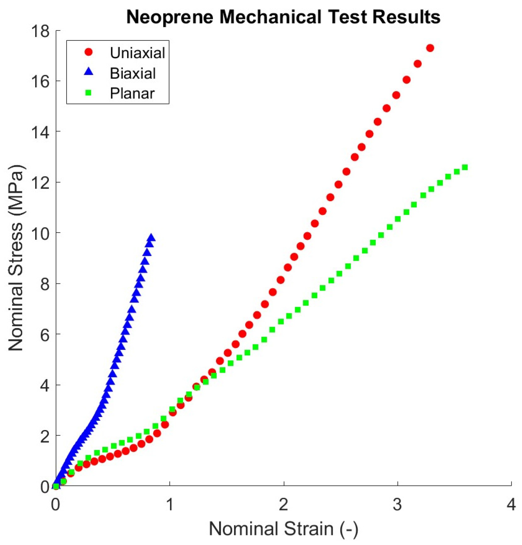
3.1. Elastomer Mechanical Test Data

The stress–strain behaviour of elastomers is typically characterised through various mechanical tests, including uniaxial tension and compression, biaxial tension, and shear testing. The experimental results used to derive the material parameters required to describe the nine material models are those produced by Beomkeun Kim [20]. Notably, the set of experimental data used in this study did not include volumetric test data because neoprene is considered nearly incompressible [20].

Three types of tests were carried out and reported, namely uniaxial tensile tests, equal biaxial tensile tests, and planar shear tests. In the uniaxial test, a dog-bone-shaped specimen was employed, and the nominal stress was computed by dividing the applied force by the original cross-sectional area of the specimen. In the case of the equiaxial tensile test, a square hook-shaped specimen was utilized, and similarly, the biaxial nominal stress was determined by dividing the applied force by the original cross-sectional area of the square hook specimen. As for the planar shear test, the testing setup resembled that of the uniaxial test, with the only difference being that the specimen’s length had to be ten times its height. The nominal stress for this test was calculated by dividing the applied force by the central section’s area.

Since there are no data for volumetric strain, a strict incompressible constraint is not enforced in the simulations. Instead, a Poisson’s ratio of approximately 0.475 to ensure efficient software operation has been assumed as suggested by the Abaqus manual. Furthermore, for most load cases, the bulk modulus had limited effect and was thus considered incompressible [1]. The nominal stress–strain curves for uniaxial, equal biaxial, and planar shear tests are illustrated in Figure 2 [20].

3.2. Test Data Fitting

Every mechanical test corresponds to a unique deformation state, a concept outlined by Beomkeun Kim [20]. These deformation states can be depicted as matrices, illustrating how material elements deform in response to varying tensile strains. In cases of mechanically uniform deformation tests, these deformation states are clearly defined. The process of curve fitting for hyperelastic material models employs optimization techniques such as least-squares minimization to identify the optimal model parameters, including stress invariants, that govern the relationship between stress and strain.

It is widely recognized that a single experiment cannot fully characterize a rubber-like material, even when assuming elasticity. As depicted in Figure 3, Figure 4 and Figure 5, even if the fitting process successfully converges for a particular mechanical test, there is no guarantee that it will accurately replicate other loading conditions using the same parameter set. The assumption of incompressibility imposes limitations on the permissible kinematic field for rubber-like materials. In the principal axes, this constraint results in all deformation conditions being determined by just two independent variables, namely, two independent stretch ratios. Consequently, relationships between equibiaxial extension and compression, as well as pure and simple shear, have already been established. Therefore, a series of biaxial tests is shown to be sufficient for a comprehensive characterization of hyperelastic constitutive models.

In this study, the Abaqus software’s built-in curve fitting algorithm, which is based on relative error minimization, was employed. The relative error is defined by Equation (19), where $T_i^{th}$ represents the nominal stress generated by the hyperelastic model, and $T_i^{Test}$ corresponds to the nominal stress derived from the test data.

$$E=\sum _{i=1}^n(1-T_i^{th}/T_i^{Test}{)}^2$$

(19)

Other than accuracy, Drucker stability needs to be considered as well. The Drucker stability criteria defines stability as a positive gradient of the nominal strain–nominal stress function [1].

3.3. Curve Fitting Results for Each Hyperelastic Model

Stress–strain predictions of each model are shown against test data in Figure 3, Figure 4, Figure 5, Figure 6 and Figure 7. The fitting quality of each hyperelastic model were determined using R² and the values are reported in each corresponding figure. Only two hyperelastic material models, namely two polynomial term and Yeoh, experienced instability.

Values of material parameters were obtained at the end of curve fitting procedures, except for the Marlow model which does not contain material parameters. Each hyperelastic model’s material parameters with values are demonstrated in

Table 1. Material parameters for each hyperelastic model.

Model Name	Material Parameters
Neo-Hookean	$C_{10}$ = 0.911, $D_1$ = 0
Mooney–Rivlin	$C_{10}$ = 0.351, $C_{01}$ = 0.644, $D_1$ = 0
Two-Term Reduced Polynomial	$C_{10}$ = 0.747, $C_{20}$ = 0.0284, $D_1$ = 0, $D_2$ = 0
Two-Term Polynomial	$C_{10}$ = 0.672, $C_{01}$ = 0.267, $C_{11}$ = −0.132, $C_{20}$ = 0.0835, $C_{02}$ = 0.0608, $D_1$ = 0, $D_2$ = 0
Yeoh	$C_{10}$ = 0.678, $C_{20}$ = 0.0592, $C_{30}$ = −0.00147, $D_1$ = 0, $D_2$ = 0, $D_3$ = 0
Arruda–Boyce	$\mu$ = 2.44, ${\lambda }_m$ = 4.50, $D$ = 0
Three-Term Ogden	${\alpha }_1$ = 0.957, ${\alpha }_2$ = 1.165, ${\alpha }_3$ = 0.744, ${\mu }_1$ = −432, ${\mu }_2$ = 211, ${\mu }_3$ = 223, $D_1$ = 0, $D_2$ = 0, $D_3$ = 0
Van der Waals	$\mu$ = 1.19, ${\lambda }_m$ = 384, $a$ = −0.594, $\beta$ = 0.318, $D$ = 0
Marlow	No Material Parameter

.

No compression nor volumetric test data were available in the literature used for this study [20]. However, these data are needed to ensure accuracy in the fitting and avoid unstable response when loaded under compression. For this reason, the compressive stress–strain curves were evaluated with negative strain values and Figure 6 and Figure 7 show the uniaxial and biaxial compression stress–strain curve of each model.

The Y axis of Figure 6 and Figure 7 use a logarithmic scale calculated with Equation (20) in order to improve the readability of the graphs.

$$Logarithmic Stress=-{\log }_{10}(-Stress)$$

(20)

4. Finite Element Analysis

Numerical Simulations Setup

To assess if stress–strain response from FEA is consistent with material element stress–strain response, for each hyperelastic model, three homogeneous deformation simulations were carried out. This is in order to assess the consistency between material model predicted stresses and numerical simulation stresses, especially how the simulation behaves under hyperelastic models’ instability range. In addition, FEA simulations are used to assess the accuracy of hyperelastic models and of element types under large static deformation.

Dog bone specimen for uniaxial tensile testing was modelled together with the cruciform shape for biaxial tensile stress and the uniform cross-section for in-plane shear. The numerical simulations were all implemented in Abaqus CAE and in each simulation, the different hyperelastic models with the corresponding geometry and boundary conditions were used. In physical uniaxial tensile test, the top and bottom rectangular sections are clamped by fixtures. To reproduce that in the numerical simulation, as shown in Figure 8, the top rectangular section was constrained in all directions, and bottom constrained as well, except in the Y-direction which allows movement. Reference Point 1 (RP-1) (see Figure 8) was coupled with the bottom surface of the bottom section, where displacement was applied, which will then move the whole bottom section down. Figure 9 demonstrates the numerical setup of the equal biaxial tensile simulation. The rectangular 30 mm × 10 mm sections at each end are constrained except in the traveling direction to reproduce clamping; thus, the central square section will be equally deformed in X-Y directions. Reference points were coupled with the cross-section of each rectangular section. Displacement in X and Y directions were added to these reference points to apply tensile load; the magnitude of displacement was identical in all directions. For planar shear simulation, similar to the uniaxial tensile simulation, the top and bottom of the 10 mm × 300 mm rectangular section shown in Figure 10 are constrained to reproduce fixture clamping. The 30 mm × 300 mm section, where deformation takes place, has a length ten times greater than its width as recommended by the literature. This aspect ratio allows thinning of the centre section with tensile load; thus, planar shear exists 45 degrees to the stretching direction [20].

The tetrahedral element offers an advantage for the automatic meshing of complex geometries. However, because the accuracy of the linear tetrahedral element is inferior to that of the quadratic tetrahedral element [17], using auto meshing with tetrahedral elements would typically favour the quadratic version for improved precision. Most of the existing literature has commonly employed linear hexahedral elements for numerical simulations involving small deformation scenarios, yielding accurate results.

This study also explores the performance of linear hexahedral elements in the context of large deformations and analyses the discrepancies when compared to auto meshing using quadratic tetrahedral elements. Element types selected were linear hexagonal hybrid element C3D8H and quadratic tetrahedral hybrid element C3D10H. In order to allow convergence with incompressible material during the numerical simulation, hybrid element formulation was used. Figure 11a, Figure 12a and Figure 13a show the hexahedral mesh whilst Figure 11b, Figure 12b and Figure 13b show the tetrahedral mesh used for uniaxial, biaxial, and in planar shear simulations.

5. Numerical Simulation Results

Reaction forces of each reference point (represented in each figure by the point labelled as RP) shown in Figure 8, Figure 9 and Figure 10 were recorded for each increment, and by using the reaction force divided by the original cross-section area, nominal stress can be obtained. The contour plot of deformation and strain results with different element types and material model predictions are compared. The nominal stress–strain curves from numerical simulation of each model with different element type are shown in Figure 14 and Figure 15. Each graph is referring to one of the material models considered and the simulation results from FEA are compared against the stress–strain curves from the literature.

6. Discussion

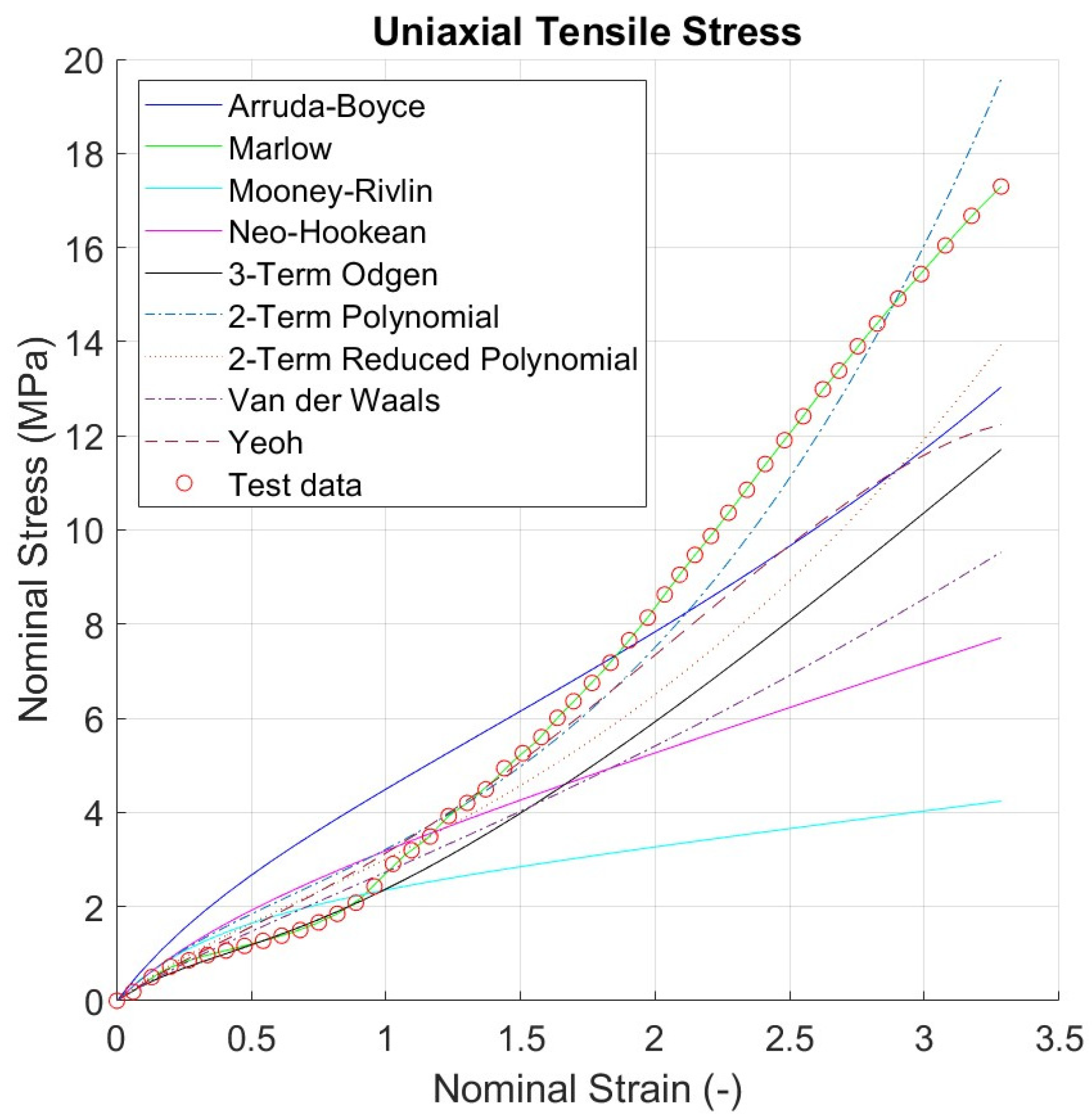
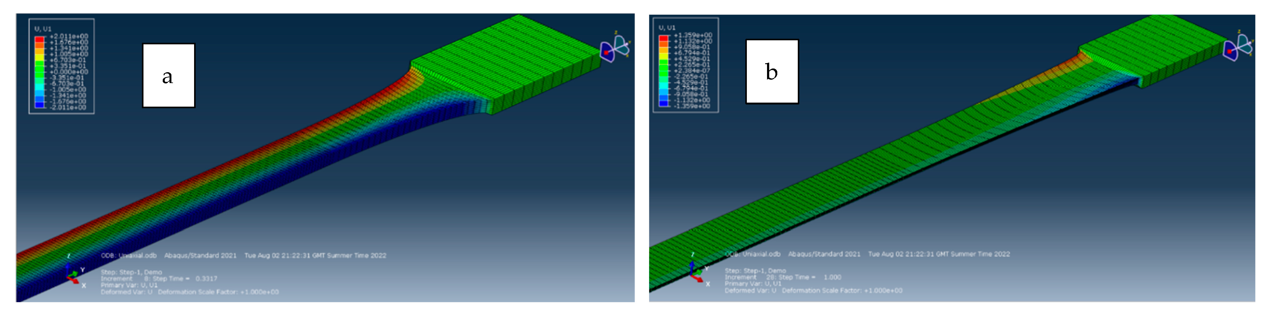
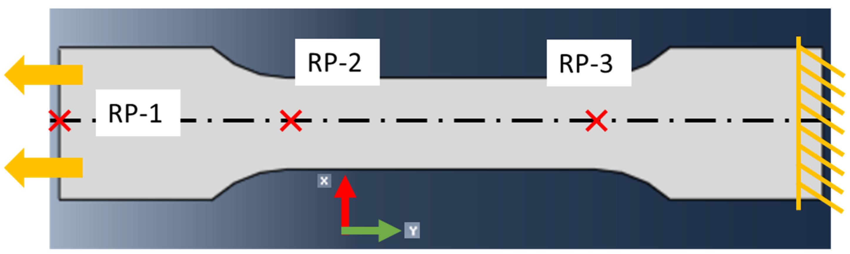
6.1. Uniaxial Tension Simulations

The results are grouped in Figure 14 and Figure 15 to show uniaxial tensile stress, where the Marlow model has a R² equal to 0.999 in uniaxial tension for both tetrahedral and hexagonal elements, suggesting that these models can replicate the material behaviour under pure tensile load independently of the element formulation. The two-terms polynomial material model has a lower R² (FEA compared with experiment) because it experiences instability when the strain value exceeds two and the stress strain curve diverged from its model prediction results (see Figure 14 and Figure 15). The contour plot illustrating longitudinal displacement in Figure 16a, corresponding to the dog bone specimen model using the two-terms polynomial material model, remains stable across the strain range under consideration and exhibits necking in the central section. As the strain range reaches the unstable range (see Figure 16b), the central section experiences an unrealistic deformation (it becomes larger) which indicates instability. The Yeoh model also showed instability, but the numerical results of the uniaxial tension load condition did not show any visible distortion at high strain. This could be explained with the strain considered in this study being within the stable range for this material model.

Comparison of the simulation results for the different models to the uniaxial tensile test data is shown in Figure 14 and Figure 15. By using the Marlow model to perform uniaxial simulation, the results match the test data in the entire strain range, and it can be considered as the most accurate model out of the nine considered in this study. It was observed that reduced polynomial and van der Waals models are stable in the strain range between 0 to 0.3, the Ogden model is stable and accurate in the strain range between 0 and 0.75, two-term polynomial and Yeoh models are accurate and stable in the strain range between 0 and 1.5, and the Marlow model is stable and accurate in the strain range between 1.5 and 3.2.

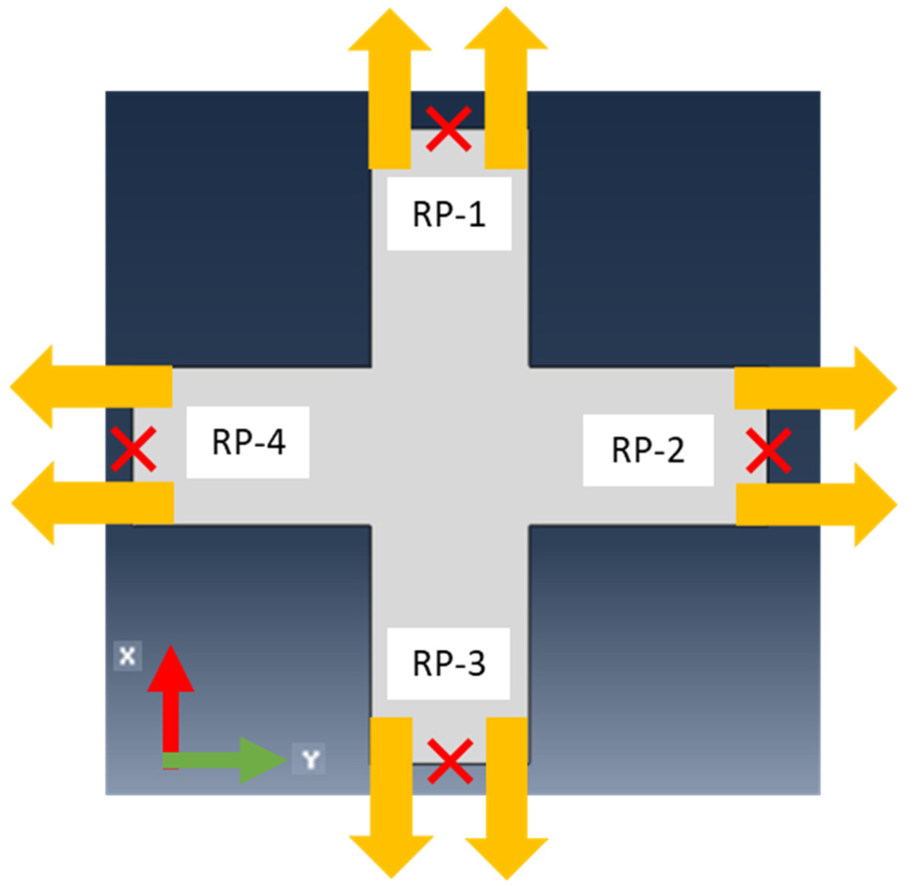
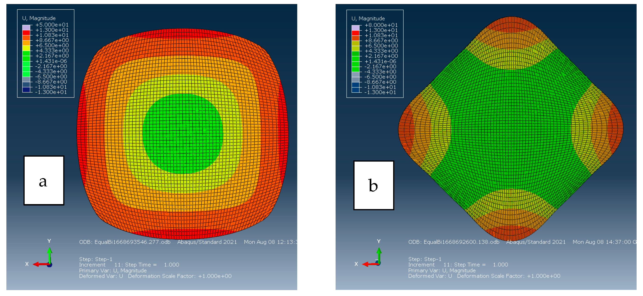
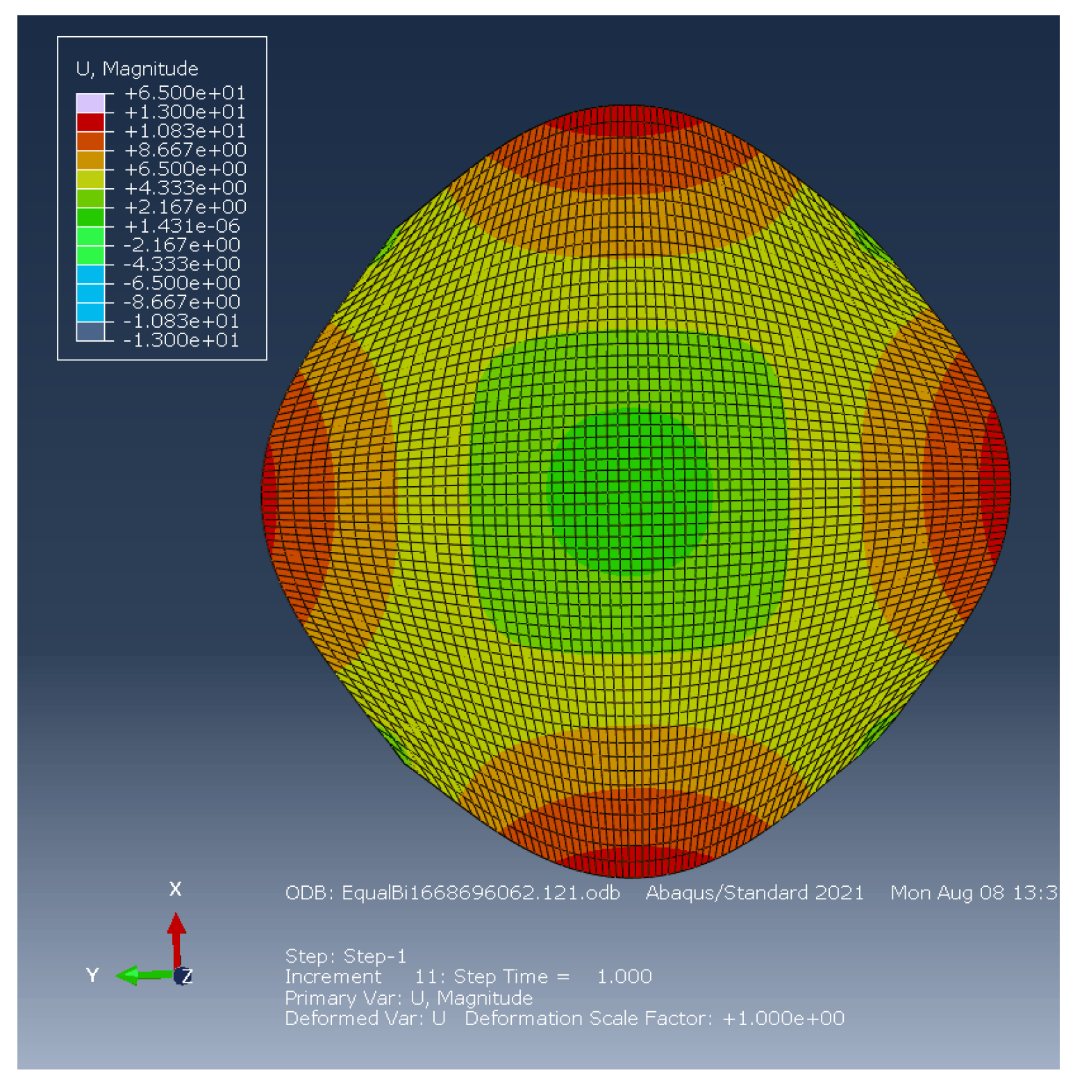
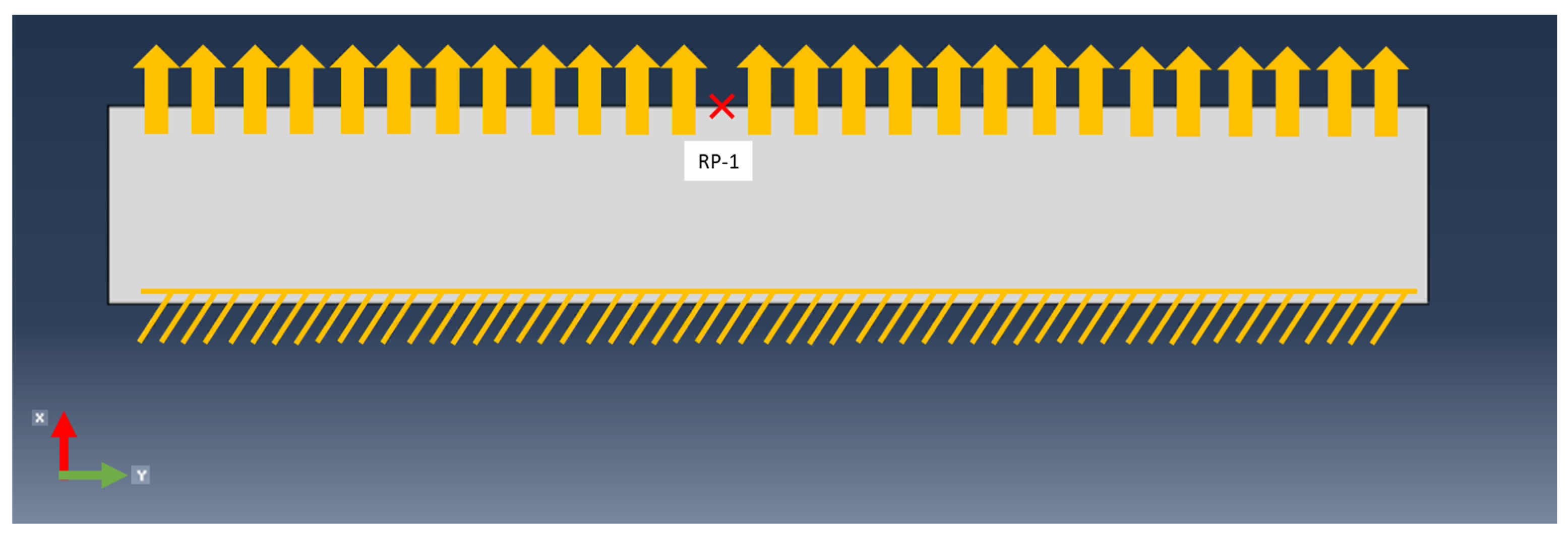
6.2. Biaxial Tensile Simulations

The simulation results for the biaxial tensile test did not follow model predictions for high strain value for most of the material models considered. This was mainly due to the shape of cruciform specimen used for the simulations of this work. The biaxial mechanical test generally uses square hook form [20] and, as demonstrated by Avanzini [21], the biaxial stress for different types of specimens would result in different model parameter values. The von Mises stress contour shown in Figure 17 highlights a stress concentration effect similar to the one observed by Avanzini [21]. The central section of the cruciform specimen cannot uniformly deform, resulting in stress levels different to those attained in square hook form. It was also observed that biaxial simulations were not converging for larger strains when tetrahedral elements and either of the models among Marlow, Mooney–Rivlin, or Yeoh were used. Moreover, the Yeoh model did not converge when hexagonal elements were used, suggesting that the model instability might contribute to the convergence issue as well.

The biaxial simulation outcomes for the two polynomial term, Mooney–Rivlin, and van der Waals models exhibited deviations from the trends predicted through curve fitting for both hexagonal and tetrahedral elements. Additionally, it was noted that the results generated by the two polynomial term model did not align with expectations due to instability. Although the Mooney–Rivlin and van der Waals models maintained stability across the entire biaxial strain range, the biaxial nominal stress derived from the simulation results, as depicted in Figure 14 and Figure 15, did not correspond to the biaxial stress observed in the experimental test data.

The deformations of the central section when applying different hyperelastic models are shown in Figure 17 and Figure 18. The displacement contour shown in Figure 18a, using the Arruda–Boyce model, shows a more uniform deformation unlike that of Mooney–Rivlin and van der Waals models (Figure 19). The non-uniform deformation of the central section was the reason why the biaxial stress calculated from simulation was diverging from model predictions, explaining why these two models were not accurate in biaxial simulation. In addition, arms of the cruciform specimen are affecting the load transfer to the central section due to the excessive deformation experienced by the arms instead of the central section [21]. Hyperelastic models which depend on the second deviatoric invariant have more unwanted deformation compared to models which only depend on the first deviatoric invariant. This suggests that for biaxial simulations like those performed in this study, the shape of the specimen should be manipulated to evaluate the biaxial accuracy of the hyperelastic models.

The comparison of the different material models predictions against the experimental results shown in Figure 14 and Figure 15 demonstrates that Marlow, Mooney–Rivlin, neo-Hookean, polynomial, reduced polynomial, van der Waals, and Yeoh models can follow the experimental results in the strain range 0 to 0.1, whilst Mooney–Rivlin, neo-Hookean, and two polynomial term models can match experimental results also in the strain range between 0.1 to 0.3.

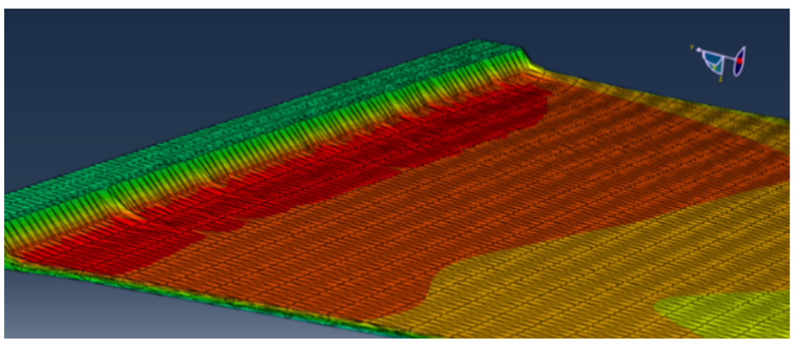
6.3. Planar Shear Simulations

Tetrahedral elements in planar shear simulation provided a close match to hexagonal elements. However, most simulations using tetrahedral elements except van der Waals and Mooney–Rivlin models did not converge in the same strain range as hexagonal elements. Comparing the deformation of the tetrahedral and hexagonal meshes shown in Figure 20 and Figure 21, an asymmetric response is observed for the tetrahedral mesh due to the asymmetric reduction in thickness. The asymmetric reduction in thickness makes the simulation converge at higher shear strain challenging. This also suggested that tetrahedral elements used to model planar shear deformation would produce unrealistic results. The hexahedral elements produced, instead, symmetric deformation and did not show any issue with convergence during simulation.

The comparison of the different material models predictions against the experimental results shown in Figure 14 and Figure 15 demonstrates that Marlow, Ogden, reduced polynomial, van der Waals, and Yeoh models can follow the experimental results in the strain range 0 to 0.5 whilst the Marlow model can match experimental results also in the strain range between 0.5 and 1, the reduced polynomial model can match also in the strain range between 1.1 and 1.6, and the two polynomial term model matches experimental results in the range 1.9 and 3.2.

7. Conclusions

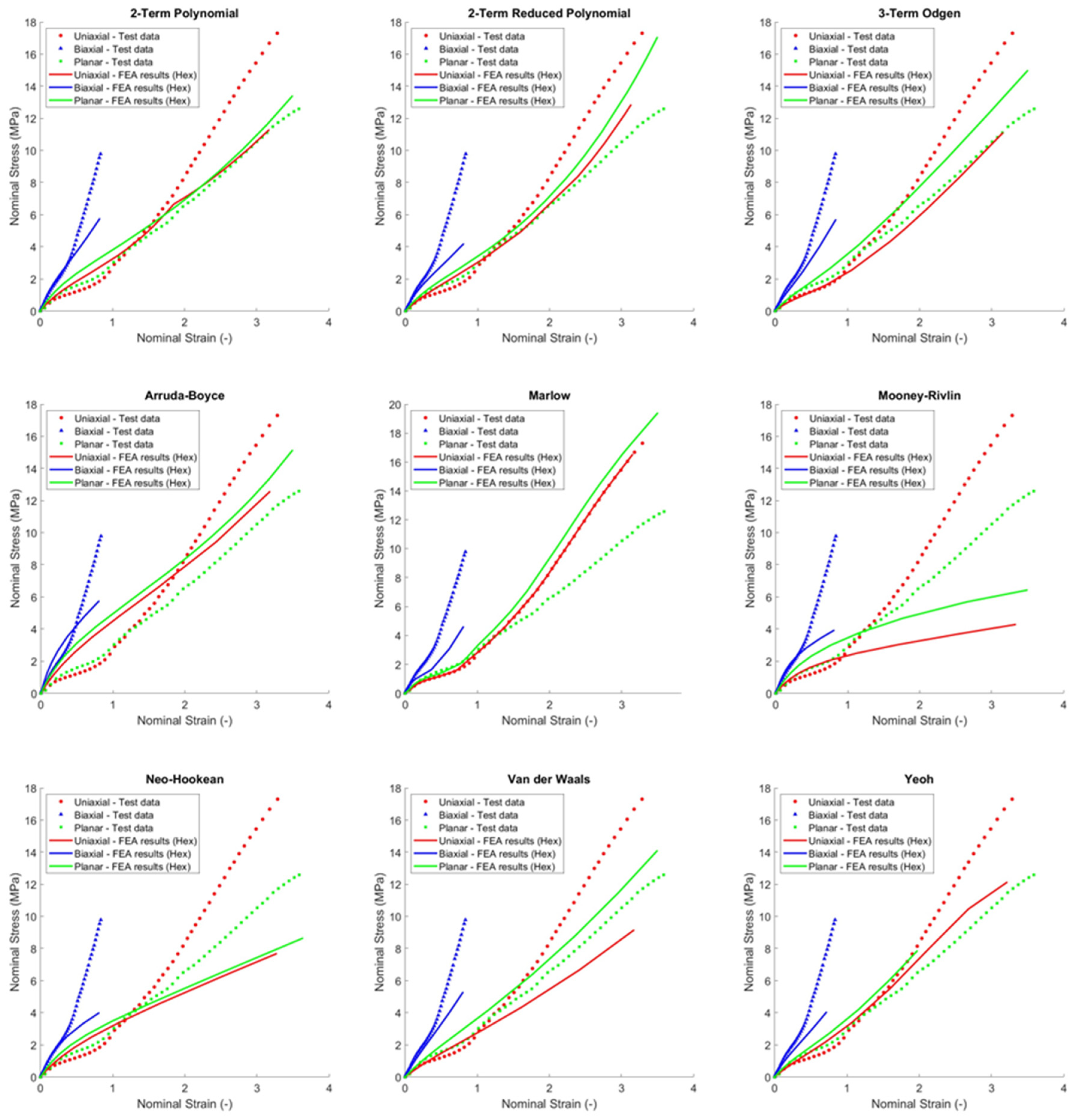
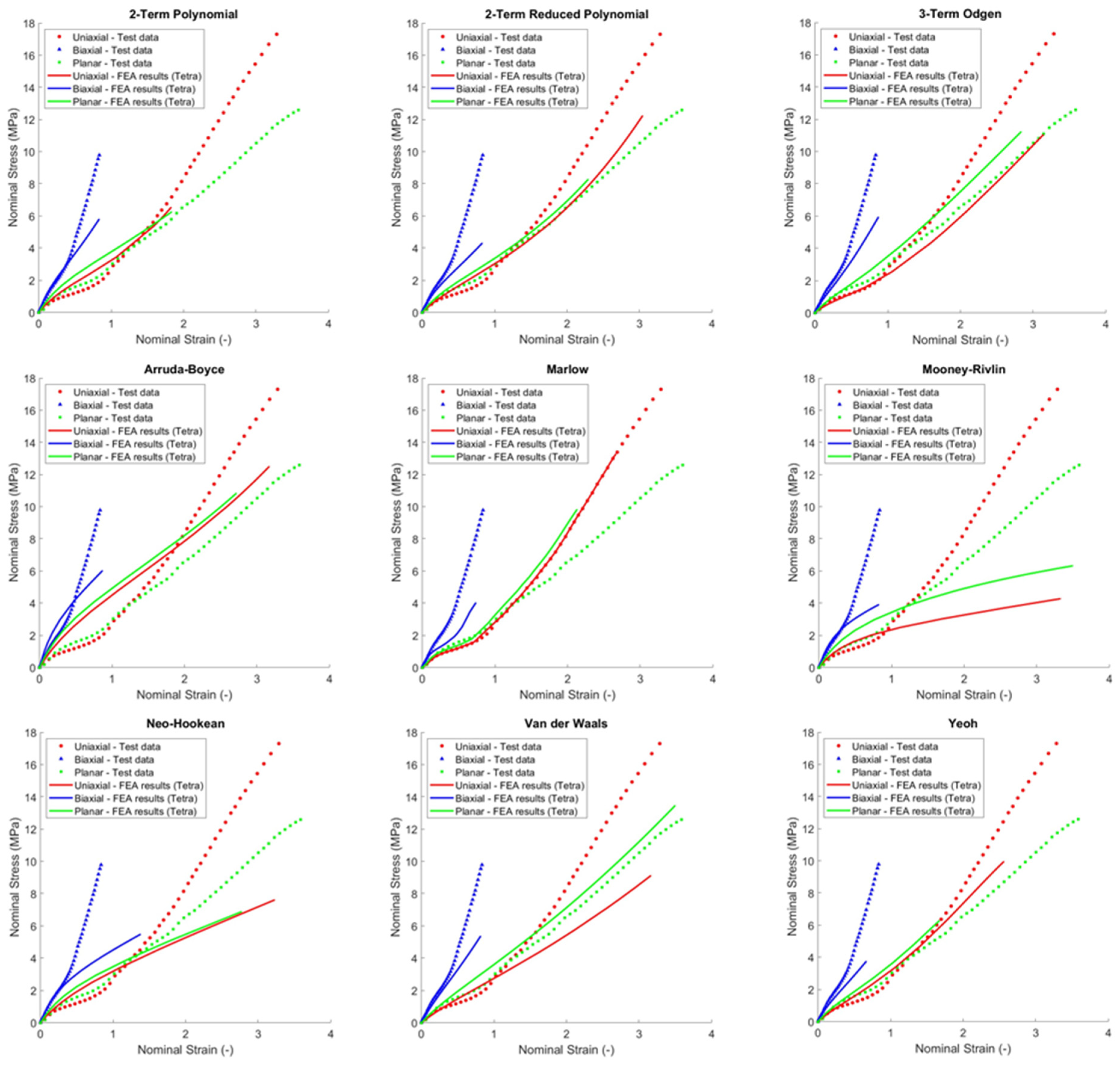
• The material parameters from each hyperelastic model were employed to create stress–strain prediction curves for the material element. Through uniaxial, biaxial, and planar shear simulations, several observations were made:
• By comparing two-term polynomial model’s uniaxial simulation results shown in Figure 14, Figure 15 and Figure 16, the Drucker’s stability of hyperelastic models emerged as a critical factor, significantly influencing the accuracy and reliability of the results.
• By comparing test data with numerical simulations results in Figure 14 and Figure 15, it became evident that each hyperelastic model can accurately describe the material behaviour in a different strain range. In particular:
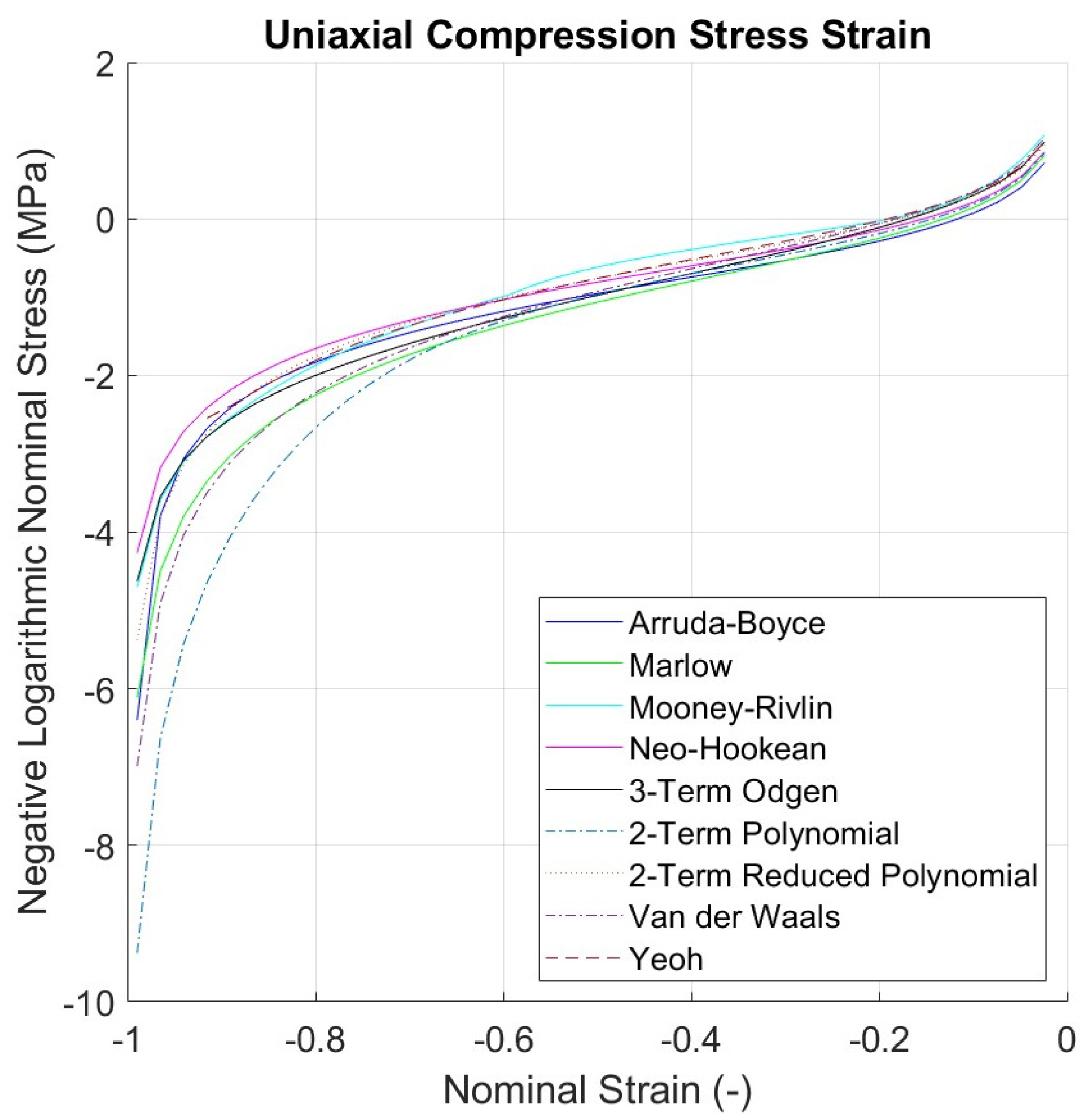
• For uniaxial tensile, reduced polynomial and van der Waals models are stable in the smaller strain range (0 to 0.3) whilst two-term polynomial and Yeoh models are stable in a larger range between 0 and 1.5.
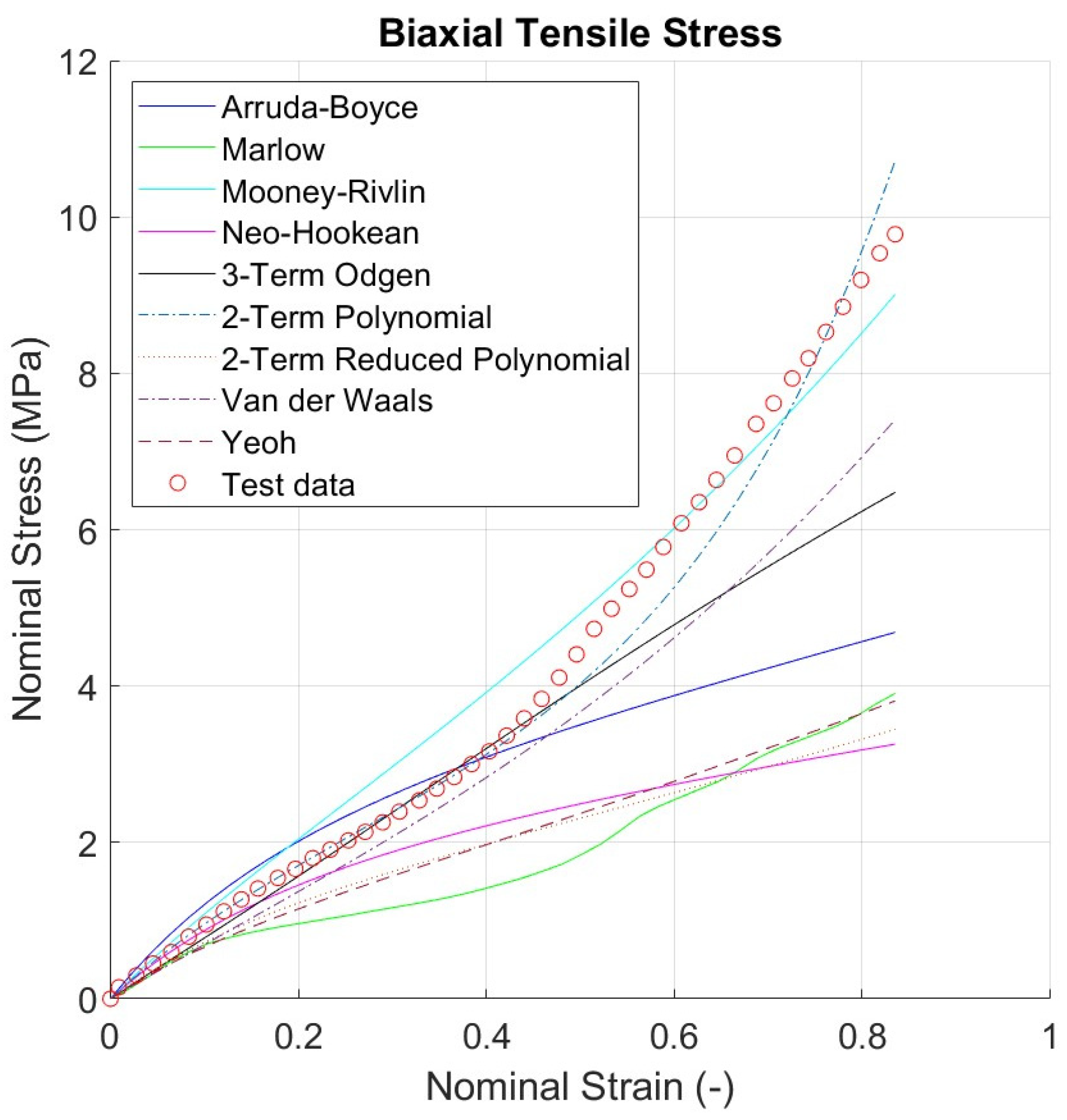
• For biaxial tensile, all the nine models investigated here can accurately predict the material behaviour up to 0.1, with Mooney–Rivlin, neo-Hookean, and two polynomial term models that can also provide an accurate response in the strain range between 0.1 and 0.3.
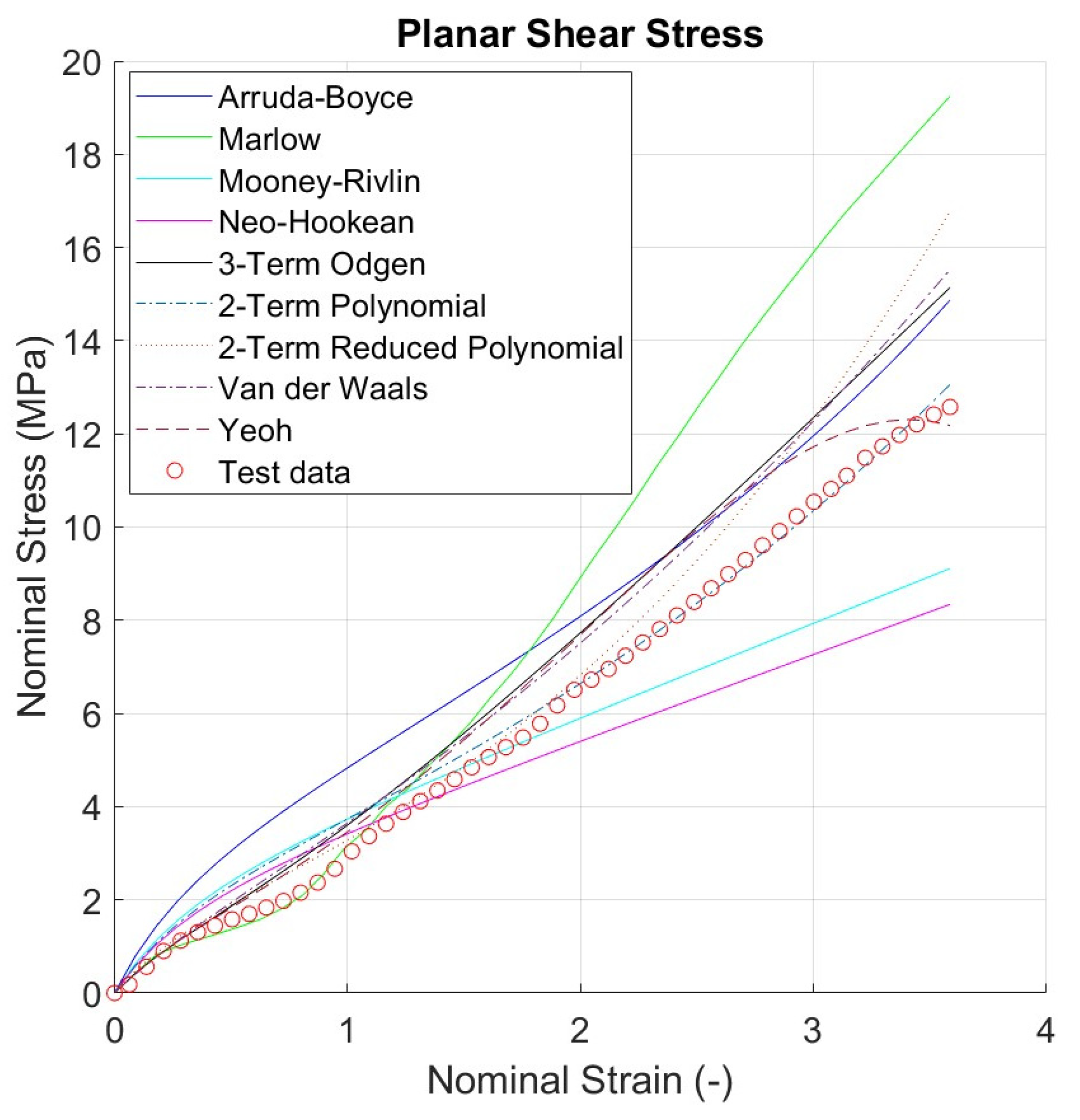
• For planar shear, all the nine models investigated here can accurately predict the material behaviour up to 0.5, with the Marlow model that can predict the response in a strain range up to 1, the reduced polynomial model that can match also in the strain range between 1.1 and 1.6, and the two polynomial term model that matches experimental results in the range of 1.9 and 3.2.
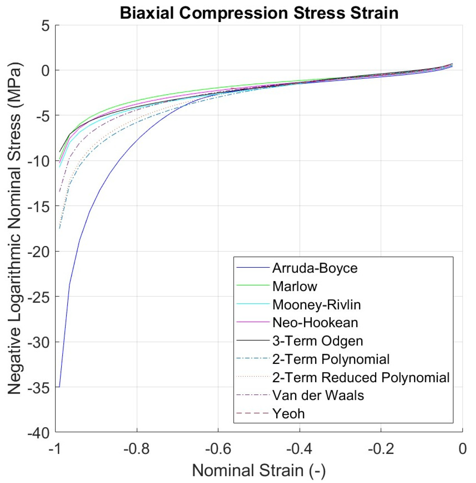
• From the biaxial simulation results shown in Figure 18 and Figure 19, it can be concluded that the geometry and configuration of the specimen used in the biaxial test dictates the maximum biaxial stress levels achievable in simulations before instability occurs. For this reason, divergence between biaxial tensile test and simulation results for biaxial strain greater than 0.3 is observed as shown in Figure 14 and Figure 15.
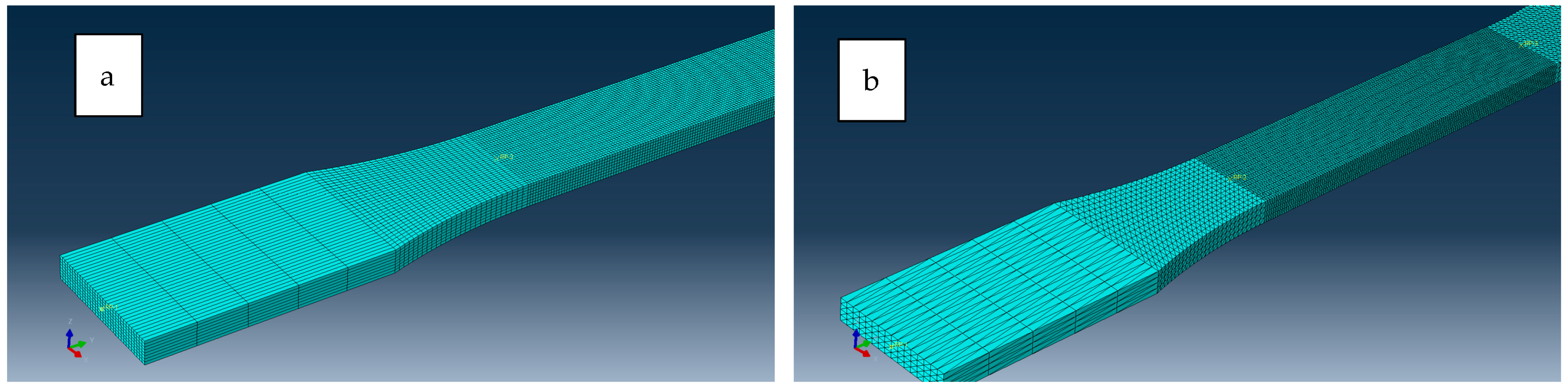
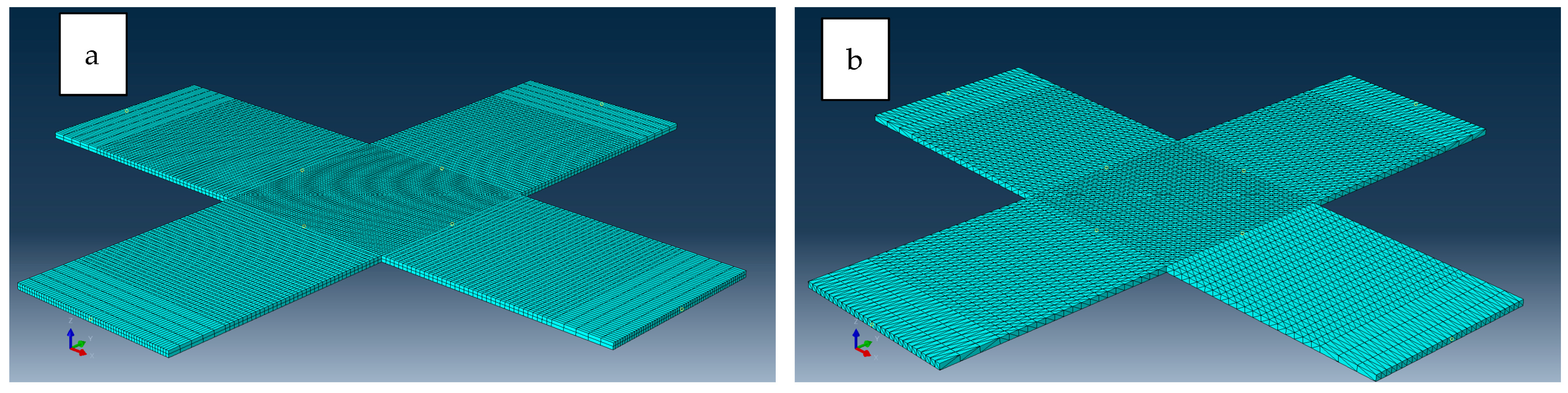
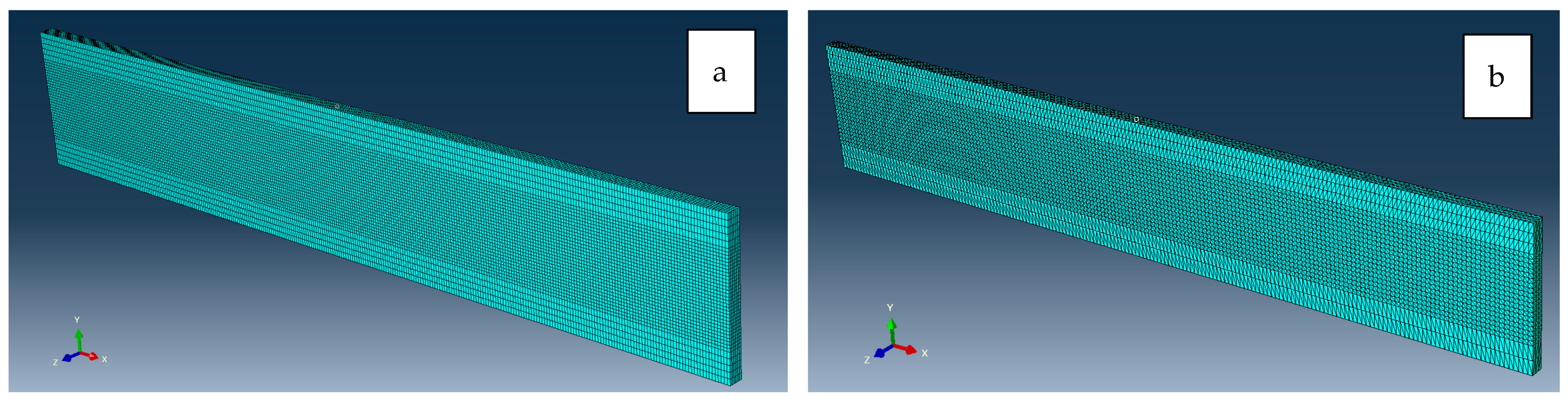
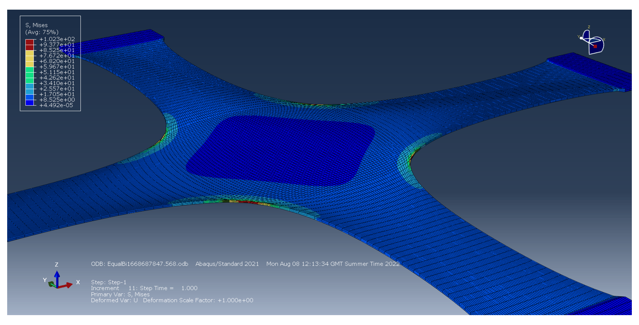
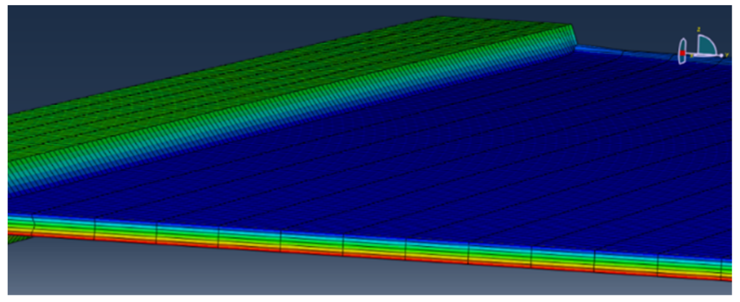
• Hexagonal elements allowed for a greater shear strain range (approximately 30% greater) compared to tetrahedral elements, as observed comparing Figure 14 and Figure 15. In addition, tetrahedral elements might pose simulation convergence challenges due to excessive distortion in higher shear strain scenarios as shown in Figure 20.

References

1. Bergstrom, J.S. Mechanics of Solid Polymers; William Andrew Publishing: Norwich, NY, USA, 2015. [Google Scholar]
2. Guo, Z.; Sluys, L.J. Constitutive Modelling of Hyperelastic Rubber-like Materials. HERON 2008, 53, 109–132. [Google Scholar]
3. Mooney, M. A Theory of Large Elastic Deformation. J. Appl. Phys. 1940, 11, 582. [Google Scholar] [CrossRef]
4. Wood, R.D. Nonlinear Continuum Mechanics for Finite Element Analysis, 2nd ed.; Cambridge University Press: Cambridge, UK, 2008. [Google Scholar]
5. Steinmann, P.; Hossain, M.; Possart, G. Hyperelastic Models for Rubber-Like Materials: Consistent Tangent Operators and Suitability for Trelor’s Data. Arch. Appl. Mech. 2012, 82, 1183–1217. [Google Scholar] [CrossRef]
6. Anandan, S.; Lim, C.Y.; Tan, B.T.; Anggraini, V.; Raghunandan, M.E. Numerical and Experimental Investigation of Oil Palm Shell Reinforced Rubber Composites. Polymers 2020, 12, 314. [Google Scholar] [CrossRef] [PubMed]
7. Wang, J.J.; Lee, J.; Woo, C.S.; Kim, B.K.; Lee, S.B. An Experimental Study and Finite Element Analysis of Weatherstrip. Int. J. Precis. Eng. Manuf. 2011, 12, 97–104. [Google Scholar] [CrossRef]
8. Luo, R.K. Complete Loading-Unloading-Deflection Prediction for Antivibration System Design Using Hyperelastic-Dissipation Approach. J. Mater. Des. Appl. 2022, 234, 859–872. [Google Scholar] [CrossRef]
9. Marckmann, G.; Verron, E. Comparison of Hyperelastic Models for Rubber-like Materials. Rubber Chem. Technol. 2006, 79, 835–858. [Google Scholar] [CrossRef]
10. He, H.; Zhang, Q.; Zhang, Y.; Chen, J.; Zhang, L.; Li, F. A Comparative Study of 85 Hyperelastic Constitutive Models for Both Unfilled Rubber and Highly Filled Rubber Nanocomposite Material. Nano Mater. Sci. 2022, 4, 65–82. [Google Scholar] [CrossRef]
11. Dal, H.; Açıkgöz, K.; Badienia, Y. On the Performance of Isotropic Hyperelastic Constitutive Models for Rubber-like Materials: A State of the Art Review. Appl. Mech. Rev. 2021, 73, 020802. [Google Scholar] [CrossRef]
12. Ricker, A.; Wriggers, P. Systematic Fitting and Comparison of Hyperelastic Continuum Models. Arch. Comput. Methods Eng. 2023, 30, 2257–2288. [Google Scholar] [CrossRef]
13. Mahnken, R. Strain Mode-Dependent Weighting Functions in Hyperelasticity Accounting for Verification, Validation, and Stability of Material Parameters. Arch. Appl. Mech. 2022, 92, 713–754. [Google Scholar] [CrossRef]
14. Anssari-Benam, A.; Horgan, C.O. A Three-Parameter Structurally Motivated Robust Constitutive Model for Isotropic Incompressible Unfilled and Filled Rubber-like Materials. Eur. J. Mech. A Solid 2022, 95, 104605. [Google Scholar] [CrossRef]
15. Jiang, M.; Dai, J.; Dong, G.; Wang, Z. A Comparative Study of Invariant-Based Hyperelastic Models for Silicone Elastomers Under Biaxial Deformation With The Virtual Fields Method. J. Mech. Behav. Biomed. Mater. 2022, 136, 105522. [Google Scholar] [CrossRef]
16. Ehret, A.E.; Stracuzzi, A. Variations on Ogden’s Model: Close and Distantrelatives. Philos. Trans. R. Soc. A Math. Phys. Eng. Sci. 2022, 380, 20210322. [Google Scholar] [CrossRef]
17. Zienkiewicz, O.C.; Taylor, R.L.; Zhu, J.Z. The Finite Element Method: Its Basis and Fundamentals, 7th ed.; Elsevier: Amsterdam, The Netherlands, 2013. [Google Scholar]
18. Bai, Y. Effect of Loading History in Necking and Fracture; Massachusetts Institute of Technology: Cambridge, MA, USA, 2008. [Google Scholar]
19. Pal, S.; Naskar, K. Machine Learning Model Predict Stress-Strain Plot for Marlow Hyperelastic Material Design. Mater. Today Commun. 2021, 27, 102213. [Google Scholar] [CrossRef]
20. Kim, B.; Lee, S.B.; Lee, J.; Cho, S.; Park, H.; Yeom, S.; Park, S.H. A Comparison among Neo-Hookean Model, Mooney-Rivlin Model, and Ogden Model for Chloroprene Rubber. Int. J. Precis. Eng. Manuf. 2012, 13, 759–764. [Google Scholar] [CrossRef]
21. Avanzini, A.; Battini, D. Integrated Experimental and Numerical Comparison of Different Approaches for Planar Biaxial Testing of a Hyperelastic Material. Adv. Mater. Sci. Eng. 2016, 2016, 6014129. [Google Scholar] [CrossRef]
Figure 1. Three types of coordinate system in the space of principal stresses [18].
Designs 07 00135 g001
Figure 2. Nominal stress–strain curves [20].
Designs 07 00135 g002
Figure 3. All hyperelastic models’ uniaxial stress prediction.
Designs 07 00135 g003
Figure 4. All hyperelastic models’ biaxial stress prediction.
Designs 07 00135 g004
Figure 5. All hyperelastic models’ planar shear stress prediction.
Designs 07 00135 g005
Figure 6. Uniaxial compression stress for all models.
Designs 07 00135 g006
Figure 7. Biaxial compression stress for all models.
Designs 07 00135 g007
Figure 8. Constraints for uniaxial tensile simulation (orange arrow indicates displacement added).
Designs 07 00135 g008
Figure 9. Constraints of the biaxial simulation (orange arrows indicate displacement added).
Designs 07 00135 g009
Figure 10. Constraints for planar shear simulation (orange arrow indicates displacement added).
Designs 07 00135 g010
Figure 11. Dog bone specimen meshed by hexagonal element (a) and tetrahedral element (b).
Designs 07 00135 g011
Figure 12. Cruciform specimen meshed by hexagonal element (a) and tetrahedral (b).
Designs 07 00135 g012
Figure 13. In plane shear specimen meshed with hexagonal element (a) and tetrahedral (b).
Designs 07 00135 g013
Figure 14. Results of numerical simulations using hexagonal element compared with test data.
Designs 07 00135 g014
Figure 15. Results of numerical simulations using tetrahedral element compared with test data.
Designs 07 00135 g015
Figure 16. Polynomial model’s dog bone necking at lower strain (a), expanding at higher strain (b).
Designs 07 00135 g016
Figure 17. von Mises stress of deformed cruciform (Arruda–Boyce model).
Designs 07 00135 g017
Figure 18. Central section deformation of Arruda–Boyce (a) and Mooney–Rivlin (b).
Designs 07 00135 g018
Figure 19. Central section deformation of van der Waals.
Designs 07 00135 g019
Figure 20. Section view of specimen with tetrahedral element using Arruda–Boyce model under shear load.
Designs 07 00135 g020
Figure 21. Section view of specimen with hexagonal element using Arruda–Boyce model under shear load.
Designs 07 00135 g021