End-to-End Deep Reinforcement Learning Control for HVAC Systems in Office Buildings

Abstract

The heating, ventilation, and air conditioning (HVAC) system is a major energy consumer in office buildings, and its operation is critical for indoor thermal comfort. While previous studies have indicated that reinforcement learning control can improve HVAC energy efficiency, they did not provide enough information about end-to-end control (i.e., from raw observations to ready-to-implement control signals) for centralized HVAC systems in multizone buildings due to the limitations of reinforcement learning methods or the test buildings being single zones with independent HVAC systems. This study developed a model-free end-to-end dynamic HVAC control method based on a recently proposed deep reinforcement learning framework to control the centralized HVAC system of a multizone office building. By using the deep neural network, the proposed control method could directly take measurable parameters, including weather and indoor environment conditions, as inputs and control indoor temperature setpoints at a supervisory level. In some test cases, the proposed control method could successfully learn a dynamic control policy to reduce HVAC energy consumption by 12.8% compared with the baseline case using conventional control methods, without compromising thermal comfort. However, an over-fitting problem was noted, indicating that future work should first focus on the generalization of deep reinforcement learning.

1. Introduction

The proper control of heating, ventilation, and air conditioning (HVAC) systems is a crucial element for reducing the amount of energy used by buildings and improving occupants’ thermal comfort [1,2]. The control of HVAC systems can usually be divided into the supervisory level and local level [3]. Supervisory-level control sets the setpoints or operation commands, whilst local-level control controls the HVAC actuators in response to supervisory-level control signals. This study focuses on supervisory-level control because of its generality. Different HVAC systems may have dramatically different local control structures due to differences in the system design, but they may share a similar supervisory control interface [3,4,5].

The most commonly found HVAC supervisory control strategy is static rule-based control, in which there is a set of if-then-else rules to determine supervisory-level setpoints or operation commands [6]. However, such simple control strategies may not achieve high HVAC energy efficiency and improved indoor thermal comfort because of the slow thermal response of buildings, dynamic weather conditions, and dynamic building internal loads [7]. Additionally, most static rule-based control strategies consider only indoor air temperature as the metric for thermal comfort, but thermal comfort is actually affected by a number of factors, including air temperature, radiant temperature, humidity, etc. [8].

1.1. Model Predictive Control

Model predictive control (MPC) has become popular over the past few years due to its potential for significant HVAC energy savings. MPC uses a building model to predict the future building performance, in which case the optimal control decisions for the current time step can be made. There have been a number of studies using MPC to control HVAC systems, such as controlling the supply air temperature setpoint for air handling units (AHUs) [9], controlling the on/off status of the HVAC system [10], controlling the ventilation airflow rates [11], and controlling zone air temperature setpoints [12], and most of them show significant energy savings.

While promising, MPC is still hard to implement in the real world because of the difficulties of HVAC modeling. The classic MPC requires low-dimensional and differentiable models; for example, the linear quadratic regulator needs a linear dynamics and quadratic cost function [13]. This is difficult for HVAC systems, especially for the supervisory control of centralized HVAC systems, not only because it has nonlinear dynamics but also because it involves a number of control logics that make it non-continuous. For example, the control logic for a single-speed direct-expansion (DX) coil may be “turn on the DX-coil if there is indoor air temperature setpoint not-met in more than five rooms”. Such logic is hard to represent with a continuous mathematical model because of the if-then-else condition. Therefore, in most previous MPC studies, either the building had an independent air conditioner for each room rather than a centralized system (such as [14,15,16]), or the MPC was used to directly control the local actuators rather than to set supervisory-level commands (such as [17,18,19]). Neither way generalizes well for typical multizone office buildings, which usually have centralized HVAC systems and non-uniform HVAC design.

To address the modeling difficulties of MPC for HVAC systems, white-box building model (physical-based model) based predictive control was proposed in [9,14,20]. This method may significantly reduce the modeling difficulties of MPC, because the white-box building model generalizes well for different buildings, and there are a number of software tools available for modeling. However, white-box building models, such as EnergyPlus models, are usually high-dimensional and non-differentiable. Heuristic search must be implemented for MPC. Given the fact that the white-box building model can be slow in computation, the scalability and feasibility of this type of MPC in the real world are questionable.

1.2. Model-Free Reinforcement Learning HVAC Control

Since model-based optimal control, such as MPC, is hard to use for HVAC systems, model-free reinforcement learning control becomes a possible alternative. To the authors’ knowledge, reinforcement learning control for HVAC systems has not yet been well studied. Either the reinforcement learning methods used are too simple to reveal their full potential, or the test buildings are too unrealistic. For example, Liu and Henze [21] applied very simple discrete tabular-setting Q-learning to a small multizone test building facility to control its global thermostat setpoint and thermal energy storage discharge rate for cost savings. Regardless of the limited real-life experiment showing 8.3% cost savings compared with rule-based control, the authors admitted that the “curse of dimensionality” of such a simple reinforcement learning method limited its scalability. In the following research by the same authors [22], a more advanced artificial neural network (ANN) was used to replace simple tabular-setting Q-learning; however, the results indicate that the use of ANN did not show clear advantages, probably due to the limited computation resources at that time.

The deep neural network (DNN) has become enormously popular lately in the machine learning community due to its strong representation capacity, automatic feature extraction, and automatic regularization [23,24,25]. Deep reinforcement learning methods take advantage of DNN to facilitate end-to-end control, which aims to use raw sensory data without complex feature engineering to generate optimal control signals that can be directly used to control a system. For example, Mnih et al. [26] proposed a deep Q-network that could directly take raw pixels from Atari game frames as inputs and play the game at a human level. More details about deep reinforcement learning can be found in Section 2.

Deep reinforcement learning methods have been widely studied not only by machine learning and robotics communities but also by the HVAC control community.

Table 1. An overview of studies focusing on deep reinforcement learning methods for HVAC systems.

Reference	Reinforcement Learning Method	Test Building	HVAC System
[27]	Linear state-value function approximation	Two buildings, each having a single zone	Independent air conditioners
[28]	Continuous-action Q-learning	Multiple apartments, each having a single zone	Independent air conditioners
[29]	Continuous-action Q-learning	A hall with multiple single rooms	Independent air conditioners
[30]	Model-assisted fitted Q-learning	A lab room	An independent HVAC unit
[31]	Model-assisted fitted Q-learning	A single chamber	A heat pump system
[32]	Deep Q-learning	A multizone office building	A variable air volume system
[33]	Multi-branching reinforcement learning	A multizone office building	A variable air volume system
[4]	Policy gradient	A multizone office building	Radiant heating systems

summarizes the HVAC control studies performed in recent years using deep reinforcement learning. Researchers have demonstrated via simulations and practical experiments that deep reinforcement learning can improve the energy efficiency for various types of HVAC systems. However, there are sparse data describing the implementation of end-to-end control for multizone buildings. On the one hand, the test buildings in several studies, including [27,28,29,30,31], were single zones with independent air conditioners. On the other hand, conventional deep reinforcement learning methods cannot effectively solve multizone control problems. Yuan et al. [32] showed that the direct application of deep Q-learning to a multizone control problem would make the training period too long. Ding et al. [33] proposed a multi-branching reinforcement learning method to solve this problem, but the method required a fairly complicated deep neural network architecture and therefore could not be scaled up for large multizone buildings. Based on deep reinforcement learning, Zhang et al. [4] proposed a control framework for a multizone office building with radiant heating systems. In this study, however, “reward engineering” (i.e., a complicated reward function of reinforcement learning) needed to be designed to help ensure that the reinforcement learning agent could learn efficiently, in which case end-to-end control could not be achieved.

1.3. Objectives

As discussed above, conventional rule-based supervisory HVAC control often results in unnecessary energy consumption and thermal discomfort. Better supervisory control methods should be found, but model-based optimal control, such as MPC, may not be practical for multizone office buildings. While previous studies have indicated that reinforcement learning control can be promising in terms of energy savings and thermal comfort, data from these studies did not provide enough information about the implementation of end-to-end control (i.e., from raw observations to the ready-to-implement control signals) for centralized HVAC systems in multizone buildings, mainly due to the limitations of reinforcement learning methods or the test buildings being single zones with independent HVAC systems. In this study, a supervisory-level HVAC control method was developed using the deep reinforcement learning framework in order to achieve end-to-end control for a typical multizone office building with a centralized HVAC system. The performance of the proposed control method, including both learning performance and building performance, were critically evaluated. The limitations of the proposed method are discussed, and the direction of future work is proposed.

2. Background of Reinforcement Learning

2.1. Markov Decision Process

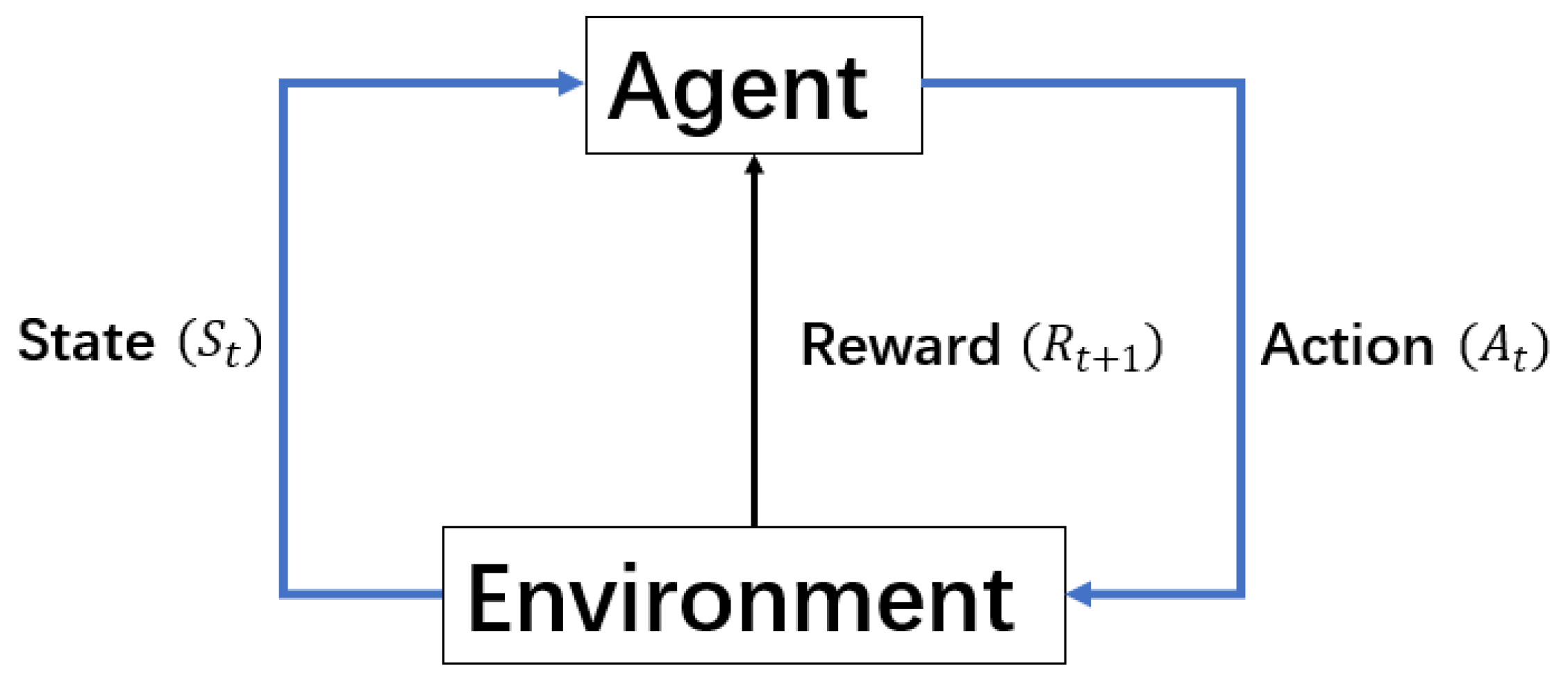
According to [34], a standard reinforcement learning problem is that a learning agent interacts with the environment in a number of discrete steps to learn how to maximize the reward returned from the environment (Figure 1). Agent–environment interactions in one step can be expressed as a tuple ($S_t$, $A_t$, $S_{t+1}$, $R_{t+1}$), where $S_t$ represents the state of the environment at time $t$, $A_t$ is the action chosen by the agent to interact with the environment at time $t$, $S_{t+1}$ is the resulting environmental state after the agent takes action, and $R_{t+1}$ is the reward received by the agent from the environment. Ultimately, the goal of reinforcement learning control is to learn an optimal policy $\pi :S_t\to A_t$ that maximizes the accumulated future reward ${\sum }_t^{T_{\infty }}{R}_t$.

The above-mentioned standard reinforcement learning problem is a Markov decision process (MDP) if it obeys the Markov property; that is, the environment’s state of the next time step ($S_{t+1}$) only depends on the environment’s state at this time step ($S_t$) and the action at this time step ($A_t$) and is not related to the state action history before this time step $t$. Most reinforcement learning algorithms implicitly assume that the environment is an MDP. However, empirically, many non-MDP problems can still be well solved by those reinforcement learning algorithms.

In reinforcement learning, there are three important concepts, including the state-value function, action-value function, and advantage function (as shown in Equations (1)–(3), where $\gamma$ is the reward discount factor) [35]. Intuitively, the state-value function represents how much reward can be expected if the agent is at state $s$ following policy $\pi$; the action-value function represents how much reward can be expected if the agent is at state $s$ taking action $a$ and then following policy $\pi$; and the advantage function, showing the difference between the action-value function and state-value function, basically indicates how good an action is with respect to the state.

$$v_{\pi }\left(s\right)={\mathbb{E}}_{\pi }\left[{\displaystyle \sum }_{k=0}^{\infty }{\gamma }^k{R}_{t+k+1}|S_t=s\right]$$

(1)

$$q_{\pi }\left(s,a\right)={\mathbb{E}}_{\pi }\left[{\displaystyle \sum }_{k=0}^{\infty }{\gamma }^k{R}_{t+k+1}|S_t=s,A_t=a\right]$$

(2)

$$a_{\pi }\left(s,a\right)=q_{\pi }\left(s,a\right)-v_{\pi }\left(s\right)$$

(3)

where ${\mathbb{E}}_{a~\pi \left(s\right)}\left[a_{\pi }\left(s,a\right)\right]=0$. For the optimal policy ${\pi }^{*}$, there is

$$v_{{\pi }^{*}}\left(s\right)=\underset{a}{\max }{q}_{{\pi }^{*}}\left(s,a\right)=\underset{a}{\max }\mathbb{E}\left[R_{t+1}+\gamma v_{{\pi }^{*}}\left(S_{t+1}\right)|S_t=s,A_t=a\right]$$

(4)

2.2. Policy Gradient

Reinforcement learning problems are usually solved by learning an action-value function $q_{\pi }\left(s,a\right)$, and the resulting policy is ${\pi }^{\prime }\left(s\right)=\arg \underset{a}{\max }{q}_{\pi }\left(s,a\right)$ if the greedy policy is used. In addition, there is another approach to reinforcement learning (known as the policy gradient) that learns the optimal policy directly without learning the action-value function. Compared with the greedy policy, the advantages of the policy gradient include better convergence properties, greater effectiveness in high-dimensional or continuous action spaces, and a better ability to learn stochastic policies [36]. The policy gradient was therefore used in this study.

The goal of the policy gradient is to learn the parameter $\theta$ in ${\pi }_{\theta }\left(s,a\right)=Pr(a|s,\theta )$ that maximizes average reward per time step $J\left(\theta \right)$, as shown in Equation (5):

$$J\left(\theta \right)={\displaystyle \sum }_s{d}_{{\pi }_{\theta }}\left(s\right){\displaystyle \sum }_a{R}_s^a{\pi }_{\theta }\left(s,a\right)$$

(5)

where $d_{{\pi }_{\theta }}\left(s\right)$ is the stationary distribution for state $s$ of the Markov chain starting from $s_0$ and following policy ${\pi }_{\theta }$, and $R_s^a$ is the reward of the agent at state $s$ taking action $a$. Gradient descent was used to maximize Equation (5). The gradient of $J\left(\theta \right)$ with respect to $\theta$ is shown in Equation (6):

$$\begin{array}{ll}{\nabla }_{\theta }J\left(\theta \right)& ={\displaystyle \sum _s}{d}_{{\pi }_{\theta }}\left(s\right){\displaystyle \sum _a}{R}_s^a{\pi }_{\theta }\left(s,a\right)\frac{{\nabla }_{\theta }{\pi }_{\theta }\left(s,a\right)}{{\pi }_{\theta }\left(s,a\right)}\\ & ={\displaystyle \sum _s}{d}_{{\pi }_{\theta }}\left(s\right){\displaystyle \sum _a}{R}_s^a{\pi }_{\theta }\left(s,a\right){\nabla }_{\theta }\log {\pi }_{\theta }\left(s,a\right)\end{array}$$

(6)

According to the policy gradient theorem, Equation (6) can be rewritten as:

$${\nabla }_{\theta }J\left(\theta \right)={\mathbb{E}}_{{\pi }_{\theta }}\left[{\nabla }_{\theta }\log {\pi }_{\theta }\left(s,a\right)q_{{\pi }_{\theta }}\left(s,a\right)\right]$$

(7)

However, $q_{{\pi }_{\theta }}\left(s,a\right)$ usually has a large variance, which may harm the convergence of the policy gradient method. To solve this problem, a baseline function $B\left(s\right)$ can be subtracted from $q_{{\pi }_{\theta }}\left(s,a\right)$ in Equation (7). Because $B\left(s\right)$ is not a function of $a$, ${\mathbb{E}}_{{\pi }_{\theta }}\left[{\nabla }_{\theta }\log {\pi }_{\theta }\left(s,a\right)B\left(s\right)\right]$ equals zero. Therefore, subtracting a baseline function from $q_{{\pi }_{\theta }}\left(s,a\right)$ does not change the expected value of Equation (7) but reduces its variance. A good choice of $B\left(s\right)$ is $v_{{\pi }_{\theta }}\left(s\right)$. Then, the new policy gradient function is:

$$\begin{array}{ll}{\nabla }_{\theta }J\left(\theta \right)& ={\mathbb{E}}_{{\pi }_{\theta }}\left[{\nabla }_{\theta }\log {\pi }_{\theta }\left(s,a\right)(q_{{\pi }_{\theta }}\left(s,a\right)-v_{{\pi }_{\theta }}\left(s\right))\right]\\ & =E_{{\pi }_{\theta }}\left[{\nabla }_{\theta }\log {\pi }_{\theta }\left(s,a\right)a_{{\pi }_{\theta }}\left(s,a\right)\right]\end{array}$$

(8)

The policy gradient in the form of Equation (8) is called advantage actor critic (A2C), which is the main reinforcement learning method used in this study.

2.3. Deep Reinforcement Learning

The size of the state space of the reinforcement learning problem can easily be very large for real-life problems. Simple tabular settings, i.e., using a lookup table to store the state values and action values for every state and every action, cannot work for a large discrete state space or a continuous state space. Instead, the value functions and policy can be estimated using the function approximation, i.e., $v_{\pi }\left(s,\theta \right)$, $q_{\pi }\left(s,a,\theta \right)$, and $\pi \left(s,a,\theta \right)$, where state values, action values, and policy are a function with respect to $\theta$. If a deep neural network is used as the function approximation, then it is called deep reinforcement learning.

The advantages of a deep neural network are its representation capacity, automatic feature extraction, and good generalization properties. Therefore, complicated feature engineering and results post-processing are no longer needed, making end-to-end control possible.

3. Methodology

Model-free deep reinforcement learning was used in this study, where the reinforcement learning agent interacted with the simulated building model offline to learn a good control policy and then controlled the real building online [21]. Since the building model was used as a simulator offline, slow computation and a non-differentiable model were no longer problems. EnergyPlus (Version 8.6 developed by the National Renewable Energy Laboratory, Golden, CO, USA) was used as the building simulation engine [37].

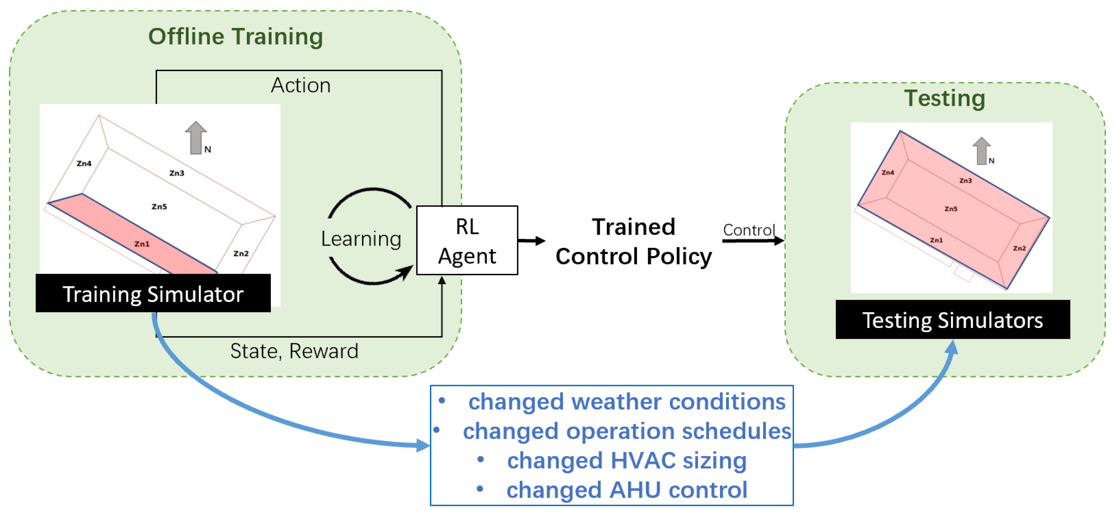
As shown in Figure 2, a multizone building simulator was used for offline model-free reinforcement learning (training), but only one zone was used as the training simulator. After learning, a control policy was obtained, and this control policy was used to control all zones in the testing simulator. Note that the testing simulator had perturbations to ensure the fairness of testing. The details of the simulators and perturbations can be found in Section 4.1.

3.1. State, Action, and Reward Design

For reinforcement learning, state, action, and reward design are critical for learning convergence (as described in Section 2.1). To take advantage of the deep reinforcement learning method, only raw observable or controllable parameters for our state, action, and reward design were used, with no extra data manipulation.

3.1.1. State

The state included the current time step’s weather conditions, the environmental conditions of the controlled zone, and the HVAC power demand, which are summarized in

Table 2. A description of the states selected for reinforcement learning.

State	Remarks
Weather conditions
Site outdoor air dry-bulb temperature	Unit: °C
Site outdoor air relative humidity	Unit: %
Site wind speed	Unit: degree from north
Site diffuse solar radiation rate	Unit: W/m2
Site direct solar radiation rate	Unit: W/m2
Zone environmental conditions
Zone thermostat heating setpoint temperature	Unit: °C
Zone thermostat cooling setpoint temperature	Unit: °C
Zone air temperature	Unit: °C
Zone air relative humidity	Unit: %
Occupancy-related zone average predicted percentage of dissatisfied using Fanger model	Unit: %, hereafter called OPPD. If the zone occupancy status is 0, OPPD is 0; otherwise, OPPD is the Fanger model predicted percentage of dissatisfied
Zone occupancy status	1 or 0
HVAC power demand
Total HVAC power demand	Unit: W, hereafter called EHVAC. EHVAC is the total electric power demand for the whole HVAC system.

.

Each item in the state should be normalized to between 0 and 1 for the optimization purpose of the deep neural network. Min–max normalization was used (as shown in Equation (9)), with the parameter’s physical limits or the parameter’s expected bounds as the min–max values. For example, the min–max values for relative humidity (%) were 0 and 100, and the min–max values for zone air temperature (°C) were 15 and 30. The temperature range was selected based on data in the literature [9,38], which shows that the typical range of setpoint temperatures for office buildings in Pennsylvania, USA, is 15 °C to 30 °C.

$$x_{norm}=\frac{x-x_{min}}{x_{max}-x_{min}}$$

(9)

3.1.2. Action

The control action of the agent was discrete and was designed as the adjustment to the last time step’s air temperature heating and cooling setpoints in the controlled zone. There are four basic action types, including:

• [0.0, 0.0] means no change to the last time step’s zone air temperature heating and cooling setpoints.
• [+deltaValue, +deltaValue] means add deltaValue to both the zone air temperature heating and cooling setpoints of the last time step. This basically means that the zone needs more heating. Note that deltaValue should be greater than zero.
• [−deltaValue, −deltaValue] means subtract deltaValue from both the zone air temperature heating and cooling setpoints of the last time step. This basically means that the zone needs more cooling. Note that deltaValue should be greater than zero.
• [−deltaValue, +deltaValue] means subtract deltaValue from the zone air temperature heating setpoint of the last time step and add deltaValue to the zone air temperature cooling setpoint of the last time step. This basically means that the zone needs no air conditioning. Note that deltaValue should be greater than zero.

The value of deltaValue is a tunable parameter, and the action space can consist of the basic action types with different deltaValue simultaneously. In Section 4, different action spaces were tested based on the four basic action types. Note that the maximum setpoint value and the minimum setpoint value were enforced to be 30 °C and 15 °C, respectively.

3.1.3. Reward

The objective of the control method is to minimize the HVAC energy consumption and thermal discomfort. Therefore, a convex combination of the OPPD and EHVAC was used as the reward (both OPPD and EHVAC here are min–max-normalized scalars):

$$-\left(\lambda \ast a+\left(1-\lambda \right)\ast EHVAC\right), where a=\{\begin{array}{cc}OPPD& OPPD\le Lm{t}_{ppd}\\ 1.0& OPPD>Lm{t}_{ppd}\end{array}$$

(10)

$\lambda$ is a tunable parameter representing the relative importance of HVAC energy efficiency and indoor thermal comfort, and $\lambda \in \left[0,1\right]$. $Lm{t}_{ppd}$ is also a tunable parameter to penalize a large OPPD. Specifically, $Lm{t}_{ppd}$ is a hyperparameter to control the penalty level for thermal discomfort. For example, if $Lm{t}_{ppd}$ is 0.15, this means that the penalty for thermal discomfort will be amplified to the maximum if OPPD is larger than 0.15. Different values of $\lambda$ and $Lm{t}_{ppd}$ were tested, as described in Section 4.4.1, to evaluate the effects of $\lambda$ and $Lm{t}_{ppd}$ on control performance.

3.2. Asynchronous Advantage Actor Critic (A3C)

Policy gradient, as discussed in Section 2.2, was the main reinforcement learning training method used in this study. Specifically, a state-of-the-art deep reinforcement learning variation of A2C, asynchronous advantage actor critic (A3C) [39], was used. In the A3C method, rather than having only one agent to interact with the environment, a number of agents interact with copies of the same environment independently but update the same global action-value or policy function network asynchronously. Still asynchronously, the agents update their own action-value or policy function network to be the same as the global one in a certain frequency. The purpose of this method is to ensure that the tuples ($S_t$, $A_t$, $S_{t+1}$, $R_{t+1}$) used to train the global network are roughly independent. Compared with the non-asynchronous methods, A3C significantly reduces the memory usage and training time cost. Details of the algorithm can be seen in Algorithm S3 of [40].

To solve the reinforcement learning problem using the advantage actor critic method, we should have two deep neural networks: one is ${\pi }_{\theta }\left(s,a\right)$ to approximate the policy, and the other is $v_{{\theta }_v}\left(s\right)$ to approximate the state-value function. Therefore, according to Equations (4) and (8), $\theta$ can be learned by gradient descent, which is:

$$\begin{gathered} \theta \leftarrow \theta +\alpha {\mathbb{E}}_{{\pi }_{\theta }}\left[{\nabla }_{\theta }\log {\pi }_{\theta }\left(s,a\right)(q_{{\pi }_{\theta }}\left(s,a\right)-v_{{\theta }_v}\left(s\right))\right] \\ =\theta +\alpha {\mathbb{E}}_{{\pi }_{\theta }}\left[{\nabla }_{\theta }\log {\pi }_{\theta }\left(s,a\right)\left(R^{\prime }+\gamma v_{{\theta }_v}\left(s^{\prime }\right)-v_{{\theta }_v}\left(s\right)\right)\right] \end{gathered}$$

(11)

${\theta }_v$ can also be learned using stochastic gradient descent with the mean squared loss function, which is:

$$\begin{gathered} {\theta }_v\leftarrow {\theta }_v-\alpha {\mathbb{E}}_{{\pi }_{\theta }}\left[\partial {\left(v_{true}-v{\theta }_v\left(s\right)\right)}^2/\partial {\theta }_v\right] \\ ={\theta }_v-\alpha {\mathbb{E}}_{{\pi }_{\theta }}\left[\partial {\left(R^{\prime }+\gamma v_{{\theta }_v}\left(s^{\prime }\right)-v{\theta }_v\left(s\right)\right)}^2/\partial {\theta }_v\right] \end{gathered}$$

(12)

In Equations (11) and (12), $\alpha$ is the step size for gradient descent, $R^{\prime }$ is the actual reward at state $s$ taking action $a$, and $s^{\prime }$ is the next state from state $s$ taking action $a$.

4. Experiments and Results

4.1. Training and Testing Building Models

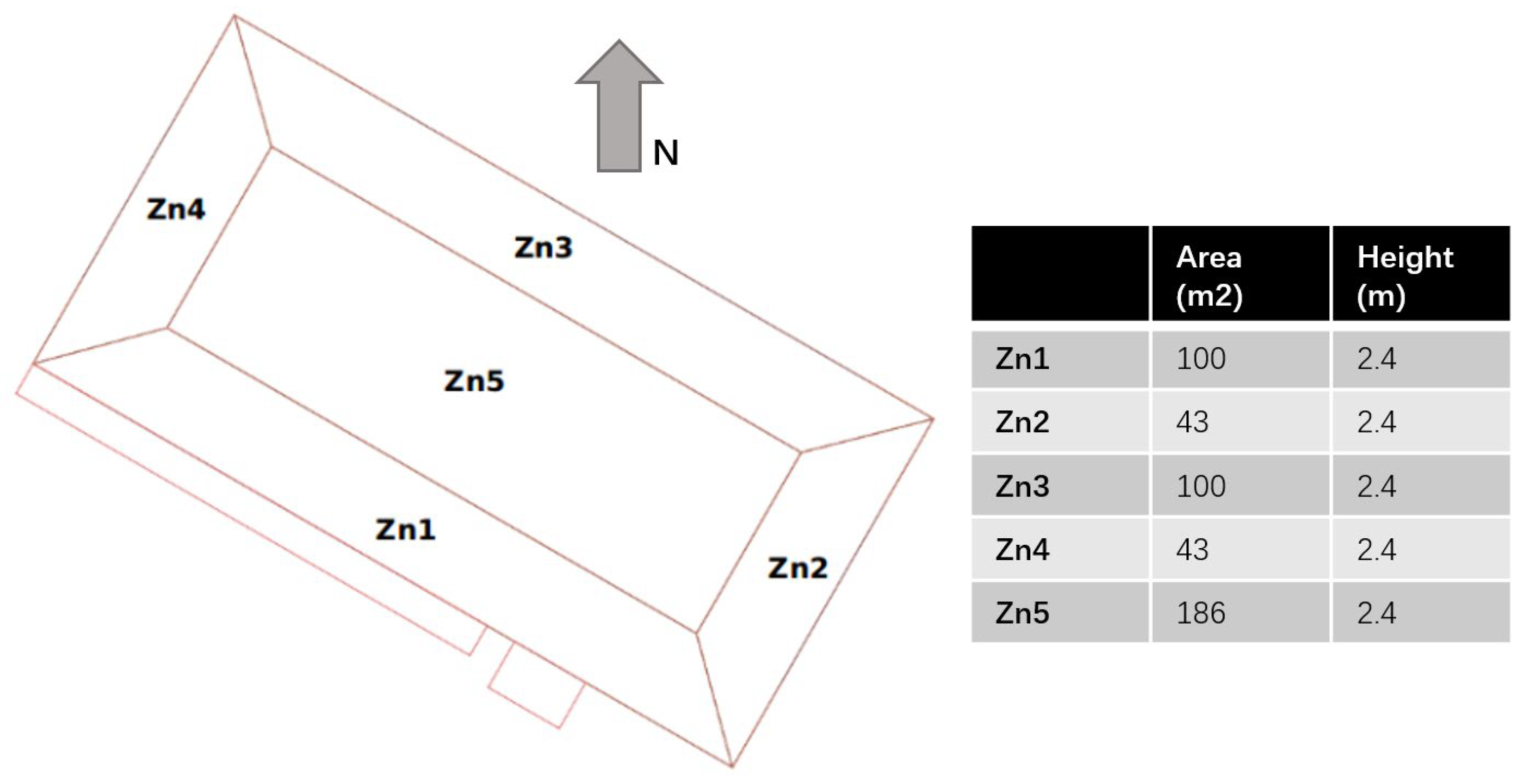
Experiments were carried out based on EnergyPlus (version 8.6, developed by the National Renewable Energy Laboratory, Golden, CO, USA) simulations. The target building in this study was selected based on the EnergyPlus v8.6 “5ZoneAutoDxVAV” example file, and Pennsylvania, USA, was selected as the location of the building due to better access to data about the environmental conditions of this site. The building was a single-level five-zone office building, the plan and dimensions of which can be seen in Figure 3. The types of building fabrics, along with their thermal properties, can be seen in

Table 3. The type of building fabrics, along with their thermal properties.

	Type	U-Value (W/m2K)	Solar Heat Gain Coefficient
External walls	Mosaic tiles (0.005 m) + heavy concrete (0.203 m) + mass wall insulation (0.049 m) + gypsum plaster (0.013 m)	1.1
Roof	Concrete tiles (0.025 m) + asphalt (0.020 m) + cement (0.050 m) + concrete (0.150 m) + insulation (0.100 m) + gypsum plaster (0.010 m)	0.42
Ground floor	Floor tiles (0.005 m) + gypsum plaster (0.0127 m) + concrete (0.150 m)	4.25
Windows	Clear glass (0.003 m) + air (0.013 m) + clear glass (0.003 m)	1.25	0.76

. The building had four exterior zones and one interior zone. All zones were regularly occupied by office workers. Each zone had a 0.61 m high return plenum. Windows were installed on all four facades, and the south-facing facade was shaded by overhangs. The lighting load, office equipment load, and occupant density were 16.15 W/m², 10.76 W/m², and 1/9.29 m², respectively.

The HVAC system of the building model was a centralized variable air volume (VAV) system with terminal reheat. The cooling source in the AHU was a two-speed DX coil, and the heating source in the AHU was an electric heating coil. The terminal reheat was also an electric heating coil.

To ensure fair evaluation of the control method, two building models with several differences were developed, called the training model and the testing model. The deep reinforcement learning agent was trained using the training model. The two models shared the same geometry, envelope thermal properties, and HVAC systems. Differences between these two models are summarized in

Table 4. Differences between the training model and the testing model.

Model	Weather File	Occupant and Equipment Schedule	HVAC Sizing	AHU Control
Training	Allegheny County, PA (TMY3)	Deterministic	Oversized by 20% from EnergyPlus auto-sizing	Dynamically change the AHU supply air temperature setpoint from 12 °C to 18 °C based on the warmest zone
Testing	State College, PA (TMY3)	Stochastic	Oversized by 44% from EnergyPlus auto-sizing	Set the AHU supply air temperature setpoint to 12 °C or 18 °C based on the outdoor air temperature

. To test the building model, the weather file was changed to a place that was about 200 km away, the occupant and equipment schedules were changed to be stochastic using the occupancy simulator [41], the HVAC equipment was more over-sized, and the AHU supply air temperature setpoint control strategy was changed to be simpler.

The EnergyPlus simulator was wrapped by the OpenAI Gym [42] for the convenience of the reinforcement learning implementation. The ExternalInterface function of EnergyPlus was used for data communication between the building model and the reinforcement learning agent during the run time.

For both training and testing, the run period of the EnergyPlus models was from Jan 1st to Mar 31st, which was the period for the whole winter season for Pennsylvania, USA. The simulation time step was 5 min. Therefore, for the discrete control of reinforcement learning control, the control time step was also 5 min.

4.2. A3C Model Setup

4.2.1. Policy and State-Value Function Network Architecture

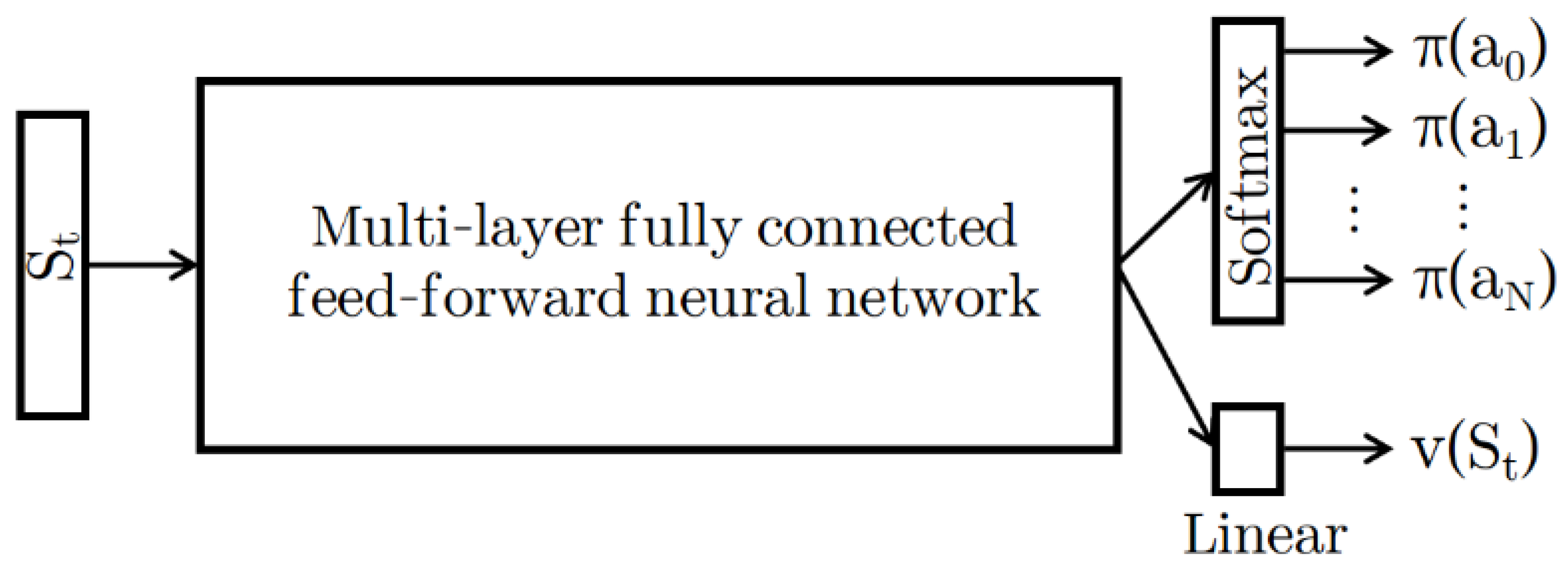
As discussed in Section 3.2, the A3C method needs two function approximation neural networks, one for the policy and the other for the state-value function. Figure 4 shows the architecture of the networks. Rather than two separate networks, a shared multilayer feed-forward neural network was used. The output from the shared network was fed into a Softmax layer and a linear layer in parallel, where the Softmax layer outputs the policy and the linear layer outputs the state value. Note that the output of the Softmax layer was a vector with the length the same as the total number of discrete actions, and each entry in the vector corresponded to the probability of taking the action.

4.2.2. Hyperparameters

The shared network of Figure 4 has four hidden layers, each of which has 512 hidden units with rectifier nonlinearity. RMSProp [43] was used for optimization, and a single optimizer was shared across all agents in A3C. The learning rate was fixed to 0.0001, and the RMSProp decay factor was 0.99. To avoid too large a gradient in gradient descent, which would harm the convergence, all gradients were clipped so that their L2 norm was less than or equal to 5.0. The total number of interactions between the A3C agents and the environment was 20 million. The entropy of policy $\pi$ was added to the policy gradient to regularize the optimization so that the agent would not overly commit to a deterministic policy in the training [44]. The weight for this regularization term was 0.01, as suggested by [40].

A building usually has slow dynamics, and the state observation of the current time step is not sufficient for the agent to make a good action choice. Recent $n$ state observations can be stacked to be the effective state observation of the agent [26]. For example, rather than just observing the current zone indoor air temperature, the agent observes the zone indoor air temperatures of current and past $n-1$ time steps to make a decision. As suggested by [26], $n$ was set to 24 in this study.

4.3. Baseline Control Strategies

The conventional fixed-schedule control strategy for indoor air heating and cooling temperature setpoints was used as the baseline. The values of the heating and cooling setpoints are usually determined by the facility manager based on experience. In this study, two sets of heating/cooling setpoints were selected, one representing the “colder” control case and the other representing the “warmer” control case.

• B-21.1: the indoor air heating and cooling setpoints were 21.1 °C and 23.9 °C from 7:00 to 21:00 (training model) or from 7:00 to 18:00 (testing model) on weekdays and 15.0 °C and 30.0 °C at all other times;
• B-23.9: the indoor air heating and cooling setpoints were 23.9 °C and 25.0 °C from 7:00 to 21:00 (training model) or from 7:00 to 18:00 (testing model) on weekdays and 15.0 °C and 30.0 °C at all other times.

It should be noted that the building model had default indoor air heating/cooling temperature setpoints, which were 21.1 °C/23.9 °C from 7:00 to 18:00 on weekdays and 7:00 to 13:00 on weekends and 12.8 °C/40.0 °C at all other times. The baseline control schedules B-21.1 and B-23.9 were only implemented when comparing them with deep reinforcement learning control. For other times, such as during the training period, the default control schedule was used. This is because the baseline schedules were manipulated to match the known building occupancy schedule, which might not be known in reality. Such manipulation was to ensure fair comparison because the proposed reinforcement learning control method had an occupancy-related control feature.

4.4. Training

The reinforcement learning agent was trained using the training building model. An 8-core 3.5 GHz computer was used to carry out the training process. The period of the training process was 5 h. In the training, it controlled the indoor air temperature heating and cooling setpoints of Zn1 (see Figure 3) only and tried to minimize the thermal discomfort of Zn1 and the HVAC energy consumption of the whole building. Therefore, as discussed in Section 3.1.1, the agent’s state observations were the weather conditions, environmental conditions of Zn1, and the whole building HVAC power demand. The reason for only controlling one zone during the training instead of controlling all five zones is to reduce the action space dimensions. The speed of convergence of deep reinforcement learning with a discrete action space relies on the action space dimension. In this study, the action space dimension increased exponentially with the increased number of controlled zones. Considering that all five zones were served by the same HVAC system and had similar thermal properties and functions, we chose to train the agent on one zone only and then applied the trained agent to all five zones to control the whole building.

4.4.1. Parameter Tuning

$\lambda$ and $Lm{t}_{ppd}$ in the reward function (see Section 3.1.3) and different combinations of deltaValue in the action space (see Section 3.1.2) were tuned. Two different values of $\lambda$ (0.4 and 0.6) were studied; three different values of $Lm{t}_{ppd}$ (0.15, 0.30, and 1.0) were studied; and two different deltaValues (1.0 and 0.5) were studied. This resulted in three action spaces:

• act1 = Zip{(0.0, 1.0, −1.0, −1.0), (0.0, 1.0, −1.0, 1.0)};
• act2 = Zip{(0.0, 1.0, −1.0, −1.0, 0.5, −0.5, −0.5), (0.0, 1.0, −1.0, 1.0, 0.5, −0.5, 0.5)};
• act3 = Zip{(0.0, 1.0, −0.5, −0.5), (0.0, 0.5, −0.5, 0.5)}.

Therefore, in total, 18 cases with different hyperparameters were trained. Each value in parentheses represents an action choice for the heating setpoint and the cooling setpoint, respectively, and the zipped tuples of both parentheses are the final action space. For example, in act1, actions include (1) no change in either the heating or cooling setpoint; (2) increase both heating and cooling setpoints by 1 °C; (3) decrease both heating and cooling setpoints by 1 °C; and (4) decrease the heating setpoint by 1 °C and increase the cooling setpoint by 1 °C. The performance of each training case was evaluated by the mean and the standard deviation of the Zn1 OPPD of occupied time steps (hereafter called OPPD Mean and OPPD Std) and the total HVAC energy consumption of the run period from 1 January to 31 March (hereafter called E_HVAC). The hyperparameters of training cases are listed in

Table 5. The training results.

	Hyperparameters			Zn1 OPPD		Building
Case	λ	Lmtppd	Acts	Mean (%)	Std (%)	EHVAC (kWh)
1	0.60	0.15	act1	6.70	2.97	5566
2	0.60	0.30	act1	8.45	6.25	5256
3	0.60	1.00	act1	9.74	6.11	5388
4	0.60	0.15	act2	6.94	2.89	5499
5	0.60	0.30	act2	7.38	4.23	5797
6	0.60	1.00	act2	7.08	4.77	5626
7	0.60	0.15	act3	9.30	6.27	5671
8	0.60	0.30	act3	7.34	4.05	7144
9	0.60	1.00	act3	8.84	4.80	5560
10	0.40	0.15	act1	7.60	3.07	5385
11	0.40	0.30	act1	10.11	6.05	5333
12	0.40	1.00	act1	10.27	7.84	5201
13	0.40	0.15	act2	7.25	3.76	5976
14	0.40	0.30	act2	8.02	4.38	5493
15	0.40	1.00	act2	8.07	4.26	5640
16	0.40	0.15	act3	6.64	3.09	5831
17	0.40	0.30	act3	9.34	5.96	5352
18	0.40	1.00	act3	9.84	6.81	5523
B-21.1	N/A	N/A	N/A	10.75	7.80	5003
B23.9	N/A	N/A	N/A	7.92	4.06	5436

Note: for all cases in this table, only Zn1 was controlled by the reinforcement learning agent or baseline control strategy; all four of the other zones were controlled using the model default control strategy.

.

4.4.2. Optimization Convergence

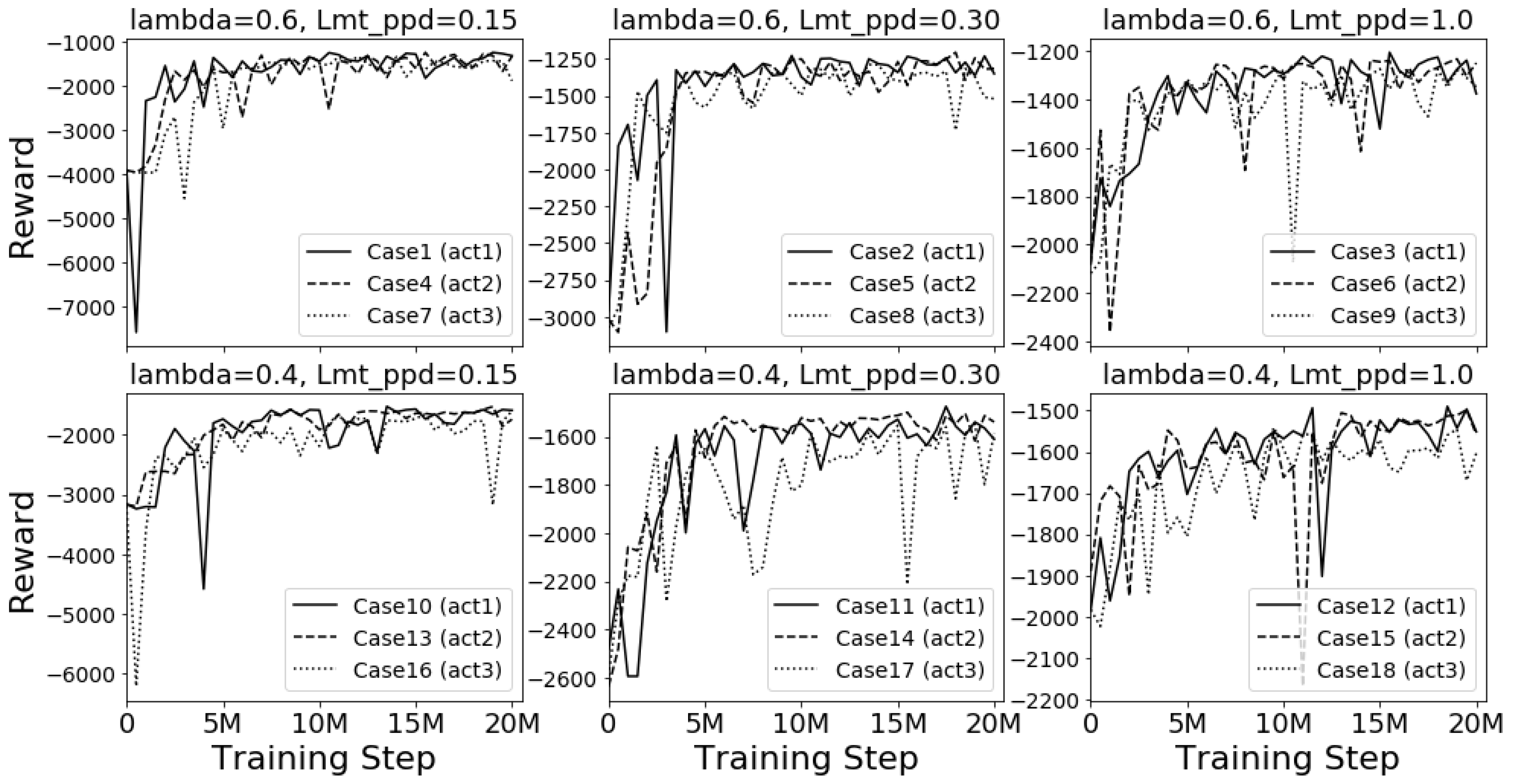
Reinforcement learning can be viewed as an optimization problem that looks for a control policy that maximizes the cumulative reward. Figure 5 shows the history of the cumulative reward for one simulation period (1 January to 31 March) for all cases in the training. Each subplot in the figure shows the reward history of cases with the same $\lambda$ and $Lm{t}_{ppd}$. Note that different subplots in the figure have different scales of the y-axis because different training cases do not share the same reward function. For the convergence study, the relative value of the reward is more important than the absolute value of the reward. It can be found that all training cases had a fairly fast convergence speed, which usually converged between 5 million and 10 million training steps. In addition, a smaller value of $Lm{t}_{ppd}$ had better convergence performance. This may be because a smaller $Lm{t}_{ppd}$, which leads to a more stringent requirement on thermal comfort, gives the agent a clearer signal about how good or how bad a state and an action are. Even though, in principle, a larger action space may take more time to converge, it is not clear in this study. It is interesting to find that the cases with $\lambda =0.6$ (larger penalty on discomfort) had better convergence performance than the cases with $\lambda =0.4$ (smaller penalty on discomfort). The reason for this difference is still not clear.

4.4.3. Performance Comparison

Table 5 shows the HVAC energy consumption and thermal comfort performance of all training cases and baseline cases. It shows that almost all training cases had less than 10% mean OPPD, and the standard deviation is fairly small. It is also found that smaller $Lm{t}_{ppd}$ is favorable because it can increase the thermal comfort performance in most cases and does not necessarily increase the HVAC energy consumption. For different $\lambda$ values, it is not expected that a smaller $\lambda$ sometimes results in increased HVAC energy consumption. It may be because, in this study, optimizing the building’s total HVAC energy consumption is difficult since the agent can only control one out of the five zones. Different action spaces were also studied, but there were no clear findings about the relationship between the action space and HVAC energy and thermal comfort performance.

Compared with the B-21.1 case, all reinforcement learning cases had better thermal comfort performance but higher HVAC energy consumption. This is as expected because the B-21.1 case had a low indoor air heating temperature setpoint. For the B-23.9 case, the comparison is more complex because some reinforcement learning cases had better thermal comfort performance and worse HVAC energy efficiency or vice versa. Among the 18 training cases, case 10 was selected as the best one compared with the B-23.9 case. Case 10 had slightly better thermal comfort performance in both the mean and standard deviation of OPPD, and it also had slightly lower HVAC energy consumption. Therefore, training case 10 was selected for the subsequent study.

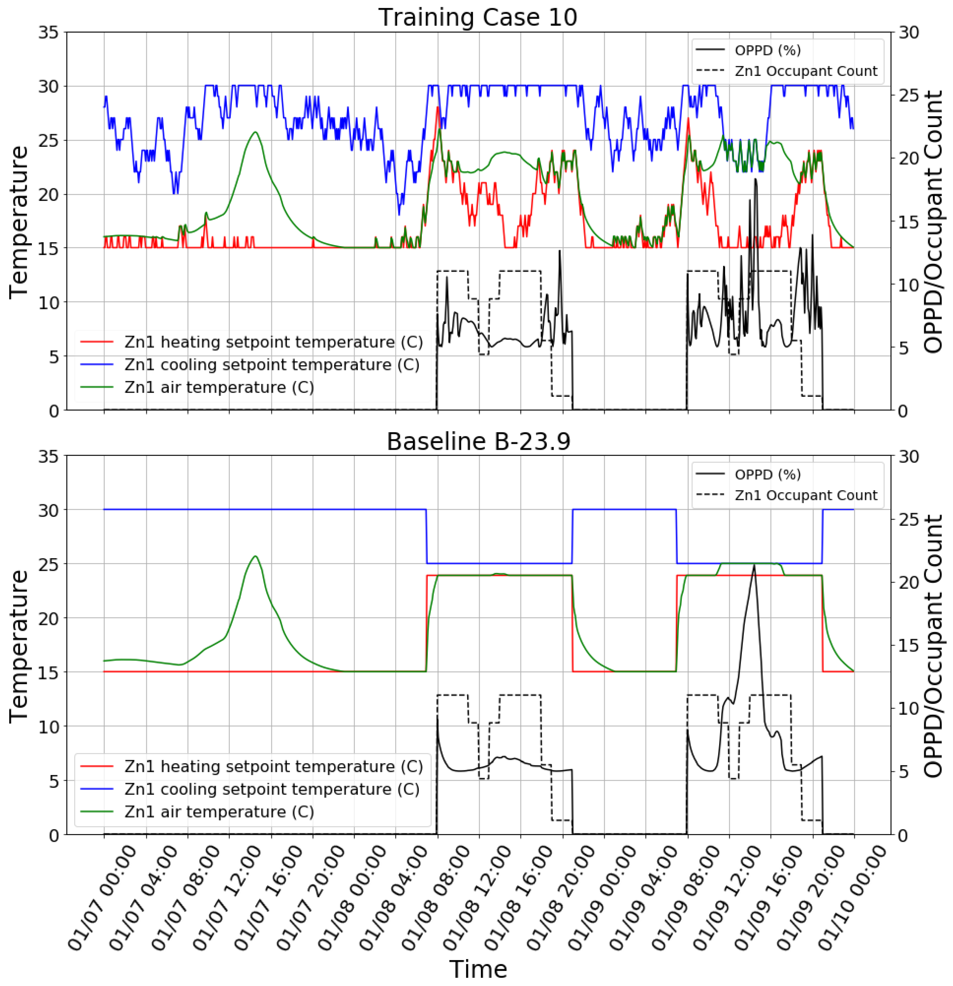
To visually inspect the learned control policy of the agent, Figure 6 shows the control behavior snapshot of the case 10 agent on three days in winter. It can be found that the agent had learned to change the setpoints according to the occupancy. Additionally, the agent had learned to preheat the space before occupants arrived in the morning. In addition, the agent could decrease the heating setpoint when the zone internal heating gain (e.g., solar heating gain) was sufficient to keep the space warm at noon and in the afternoon of the day. However, the agent did not start to decrease the heating setpoint until the zone became unoccupied. The agent had to take nearly an hour to decrease the heating setpoint to the minimum value, which wasted HVAC energy. The OPPD of training case 10 in Figure 6 was kept lower than 10% most of the time. However, it is interesting to find that the OPPD reached above 15% in the afternoon of 01/09. The primary reason is the too high mean radiant temperature of the zone caused by strong afternoon solar radiation. The agent did decrease the cooling setpoint in response to this situation, but cooling was still not enough to offset the effect of the high mean radiant temperature. This shows that the agent is not well trained to deal with this type of situation. Compared with the B-23.9 case, the reinforcement learning agent tended to overheat the space in the morning and then let the indoor air temperature float, rather than keep the heating setpoint constant. The reason is probably that the agent wants to heat the space quickly in the morning in order to create a warm environment before occupancy. There are lots of small fluctuations in heating and cooling setpoints in the reinforcement learning case because the reinforcement learning agent gives a stochastic policy rather than a deterministic one. The stochastic policy is used because it helps the agent to explore unknown states. It is easy to change the stochastic policy to the deterministic one if needed.

4.5. Testing

The trained reinforcement learning agent of training case 10 was tested in three scenarios, including single-zone testing in the testing building model, multizone testing in the training building model, and multizone testing in the testing building model. The trained agent’s performance in the testing was also evaluated by OPPD Mean, OPPD Std, and E_HVAC.

4.5.1. Single-Zone Testing in the Testing Building Model

The trained agent in training case 10 was tested using the testing building model to control Zn1 of the building model, which was the same zone that the agent was trained on. All other zones still had setpoints with the fixed schedule.

Table 6. The results of single-zone testing in the testing building model.

Case	Zn1 Mean OPPD (%)	Zn1 Std OPPD (%)	Building EHVAC (kWh)
Trained agent 10	10.57	7.65	5803
B-21.1	13.25	9.52	5550
B-23.9	8.58	7.03	5942

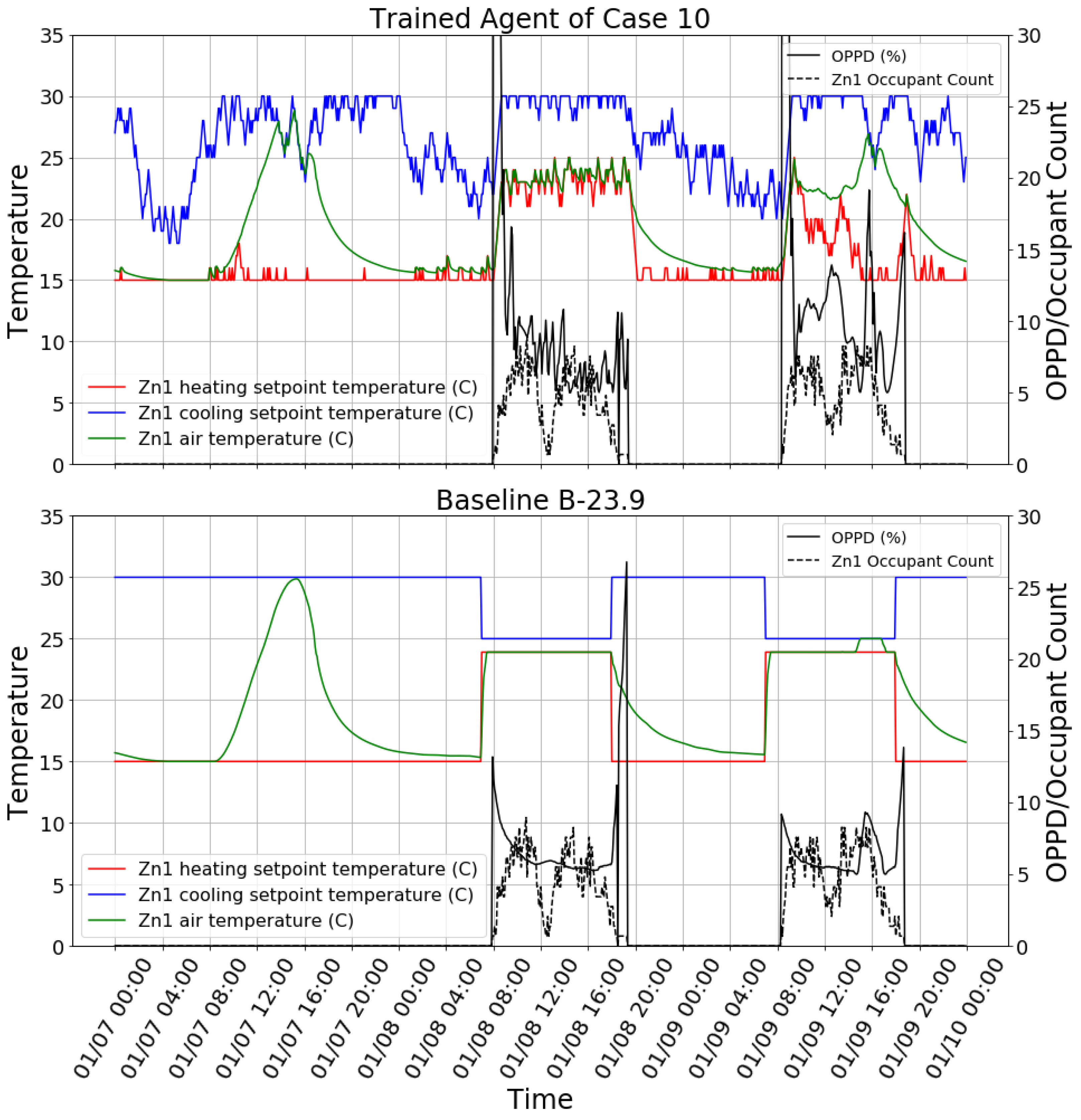
Note: For all above cases, the control strategy of all zones except for Zn1 was the default control strategy of the building model.

shows the performance comparison between the reinforcement learning agent and baseline cases. It can be found that the reinforcement learning agent had a performance between the two baseline cases: its thermal comfort performance was worse than that of B-23.9, and its HVAC energy consumption was higher than that of B-21.1. The control behavior snapshot of the reinforcement learning agent and B-23.9 is shown in Figure 7. It can be found that the agent in this testing scenario still had a reasonable control policy but did not perform as well as in the training case. Firstly, the heating setpoint was sometimes too low during the occupied time even though the zone air temperature was not warm enough, e.g., at around noon on 01/09. Secondly, the cooling setpoint was sometimes too low during the unoccupied time, which triggered the cooling of the zone, e.g., on 01/07 from 8:00 to 16:00. An interesting finding is that there was a spark on OPPD in the B-23.9 case between 01/08 18:00 and 01/08 19:00 because the schedule set the heating setpoint to 15 °C while the zone was still occupied. This did not occur in the reinforcement learning case because it takes the occupancy as an input.

4.5.2. Multizone Testing in the Training Building Model

The trained reinforcement learning agent (case 10) was tested in the training building model to control all zones rather than just one. As shown in

Table 7. The results of multizone testing in the training building model.

	Zn1 OPPD		Zn2 OPPD		Zn3 OPPD		Zn4 OPPD		Zn5 OPPD		Building
Case	Mean (%)	Std (%)	Mean (%)	Std (%)	Mean (%)	Std (%)	Mean (%)	Std (%)	Mean (%)	Std (%)	EHVAC (kWh)	Note
10-0	8.13	5.96	8.90	6.56	7.75	5.62	7.70	5.91	9.45	6.05	6983	As-is trained agent case 10
10-1	8.31	7.35	9.32	7.62	8.02	7.10	7.95	7.24	9.83	6.85	5328	Trained agent case 10 + night setback rule
10-2	10.46	11.11	9.86	9.08	9.67	10.47	9.97	11.09	10.37	8.12	4938	Trained agent case 10 + mask on state input EHVAC
B-21.1	10.79	7.86	10.33	7.44	9.89	7.73	10.25	7.88	7.29	4.16	4809	N/A
B-23.9	8.09	4.34	8.74	5.52	6.37	1.90	6.78	2.37	7.51	2.56	6109	N/A

, case 10-0 achieved good thermal comfort for all zones but consumed much more energy than the baseline cases. The high HVAC energy consumption was primarily caused by the fact that the agent sometimes increased the heating setpoint during unoccupied times. This strange behavior of the trained agent is partially because the agent over-fitted to the HVAC energy consumption pattern in the training. Two additional tests were conducted to further analyze the agent’s performance. One test used the trained agent along with a night setback rule: heating and cooling setpoints were set to 15 °C and 30 °C between 21:00 and 06:00 (case 10-1 in Table 6). The other test applied a mask to the state observation EHVAC: EHVAC was always zero in the testing (case 10-2 in Table 7). The results show that case 10-1 consumed 12.8% less HVAC energy than B-23.9 and achieved good thermal comfort performance, although not as good as B-23.9. Case 10-2 overcame the “unnecessary heating” problem of case 10-0, but it did not achieve as good a thermal comfort performance as case 10-1 because one state observation was masked. However, as expected, case 10-2 consumed even less HVAC energy consumption than case 10-1 at the price of worse thermal comfort.

4.5.3. Multizone Testing in the Testing Building Model

The trained reinforcement learning agent (case 10) was tested in the testing building model to control all zones. This is the most stringent test because both the building model and the control mode are different from the training. As shown in

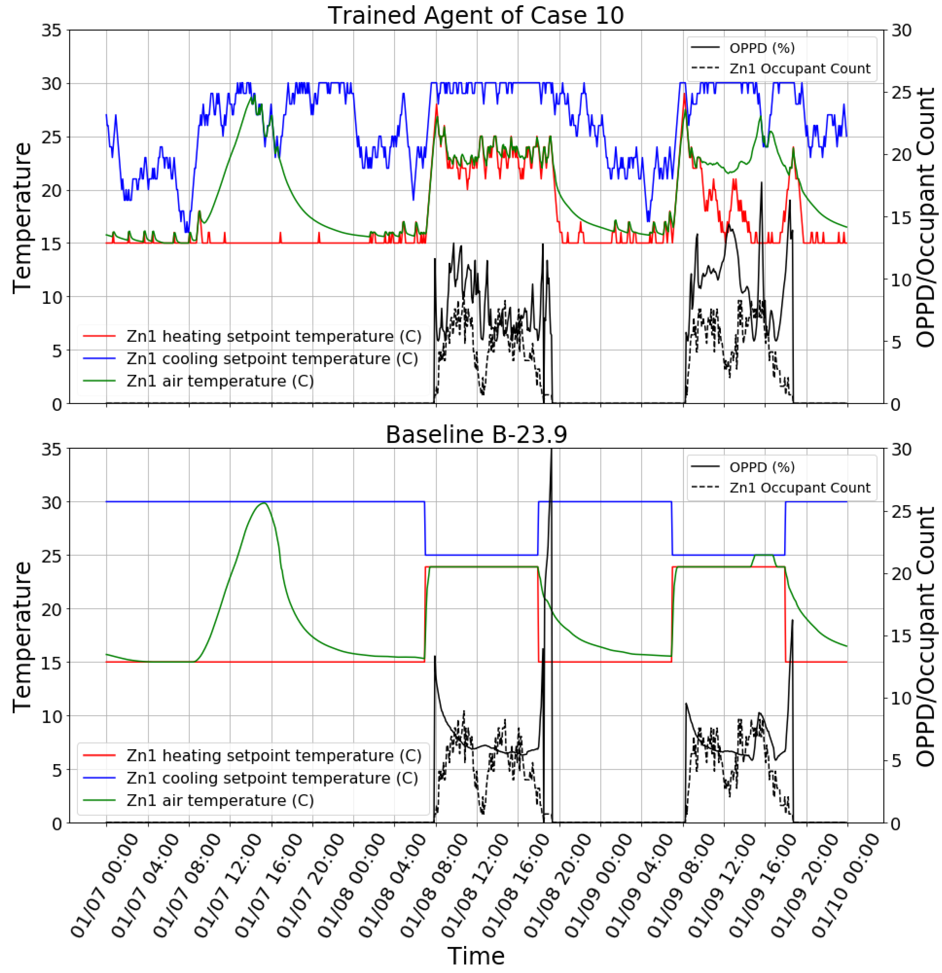
Table 8. The results of multizone testing in the testing building model.

	Zn1 OPPD		Zn2 OPPD		Zn3 OPPD		Zn4 OPPD		Zn5 OPPD		Building
Case	Mean (%)	Std (%)	Mean (%)	Std (%)	Mean (%)	Std (%)	Mean (%)	Std (%)	Mean (%)	Std (%)	EHVAC (kWh)
10	13.84	14.31	12.12	11.87	12.66	13.53	13.45	13.55	9.40	10.37	5884
B-21.1	13.24	9.52	11.67	8.52	12.18	9.45	13.24	9.38	7.98	6.84	5752
B23.9	8.54	7.00	8.99	7.17	7.10	6.54	7.76	6.79	7.57	4.88	6965

, the agent did not perform well in terms of either thermal comfort or HVAC energy efficiency. Firstly, the agent had worse thermal comfort performance than both B-21.1 and B-23.9; secondly, the agent consumed more energy than B-21.1. This means that using B-21.1 is better than using the trained agent in terms of both energy efficiency and thermal comfort. To find the reasons behind the agent’s poor performance, the control behavior snapshot of Zn1 on three days in winter is plotted in Figure 8. It is clear that, for the reinforcement learning control case, high OPPD occurred in the morning because occupants arrived earlier and the agent started to increase the heating setpoint. We calculated the value count for the time that OPPD was higher than 20% for Zn1. It shows that about 70% of the larger-than-20% OPPD samples occurred between 06:00 and 10:00 (not included). This is partially because the trained agent over-fitted to the occupancy schedule of the training building model. In the training building model, occupants arrived at exactly 08:00 every workday, but in the testing building model, a stochastic occupancy schedule was used, in which there is some possibility that occupants arrive before 08:00. One observation in favor of the agent is that the B-23.9 case may have had high OPPD in the evening because the heating setpoint was set back to 15 °C while the zone was still occupied. The agent performed better regarding this problem because it takes occupancy as one of the inputs. For the whole building, the reinforcement learning case had 17% fewer larger-than-20% OPPD samples than B-23.9 for the time between 18:00 and 21:00 (not included) during the simulation period.

4.6. Discussion

Optimization and generalization are two main problems in machine learning. Optimization is about how well the machine learning method can learn from the training data to minimize some loss functions. Generalization is about how well the trained machine learning model (or agent) performs with unseen data (or environments).

It was found in this study that the deep reinforcement learning control method had good convergence performance in the training, which usually converged long before the maximum learning step was reached. This finding is consistent with existing studies on deep reinforcement learning [4,45]. It was also found that all training cases could achieve good thermal comfort performance, and one training case was better than the B-23.9 baseline case in terms of both thermal comfort and HVAC energy efficiency. This shows that the proposed deep reinforcement learning control method could be well optimized.

Generalization performance is more difficult to evaluate for building control. Ideally, the trained agent’s performance in controlling a real building is a good evaluation method. However, in this study, no real buildings were available. Therefore, the agent was evaluated in three testing scenarios. In the first testing scenario, the trained agent was used to control the same zone as in the training but with different weather conditions, operation schedules, etc. In this case, the agent could still perform reasonably, although not as well as in the training case. The agent might over-fit to the weather conditions of the training building model if it could not provide enough heating to the zone. In the second testing scenario, the trained agent was used to control different zones from the training, but the building model was exactly the same as in the training. This case clearly shows that the trained agent over-fitted to the HVAC energy profile in the training. When forcing a night setback rule for the agent, it achieved good thermal comfort performance in all zones and saved 12.8% HVAC energy consumption compared with the B-23.9 baseline case. Thirdly, the agent was used to control different zones from those in the training, and the building model was also different. In this case, the agent did not perform well. The trained agent might have over-fitted to the occupancy schedule of the training building model. Therefore, it can be concluded that the trained agent experienced the over-fitting problem. This problem was also reported in [46,47,48].

It must be admitted that there is a lack of a systematic method to diagnose the over-fitting problem of deep reinforcement learning control. All testing scenarios in this section can only conclude that the trained agent has an over-fitting problem, and there is no strong conclusion about where it over-fits. To the authors’ knowledge, there is still no good theory behind the generalization of deep learning [49].

5. Conclusions and Future Work

Reinforcement learning control for HVAC systems has been thought to be promising in terms of achieving energy savings and maintaining indoor thermal comfort. However, previous studies did not provide enough information about end-to-end control for centralized HVAC systems in multizone buildings, mainly due to the limitations of reinforcement learning methods or the test buildings being single zones with independent HVAC systems. This study developed a supervisory HVAC control method using the advanced end-to-end deep reinforcement learning framework. Additionally, the control method was applied to a multizone building with a centralized HVAC system, which is not commonly seen in the existing literature. The control method directly took the measurable environmental parameters, including weather conditions and indoor environmental conditions, to control the indoor air heating and cooling setpoints of the HVAC system. A3C was used to train the deep reinforcement learning agent in a single-level five-zone office building model. During the training, the reinforcement learning agent only controlled one out of the five zones, with the goal of minimizing the controlled zone’s thermal discomfort and the HVAC energy power demand of the whole building.

It was shown that the proposed deep reinforcement learning control method had good optimization convergence properties. In the training, it learned a reasonable control policy for the indoor air heating and cooling setpoints in response to occupancy, weather conditions, and internal heat gains. After hyperparameter tuning, a good training case was found, which achieved better thermal comfort and HVAC energy efficiency compared with the baseline case. It was also found that the penalty on large OPPD was beneficial to convergence.

By applying the trained agent to control all five zones of the training building model, 12.8% HVAC energy savings in comparison to one baseline case was achieved with good thermal comfort performance; however, a setpoint night setback rule must be enforced for the agent because of its over-fitting problem. The agent failed to achieve good performance in terms of both thermal comfort and HVAC energy efficiency if it was applied to control all five zones of the testing building model, also due to the over-fitting problem.

Future work should first focus on generalization techniques of deep learning. Dropout or batch normalization should be first considered to reduce over-fitting. The choice of the weather and occupancy schedule for training should be performed carefully to ensure that they are representative. Feature augmentation methods can be considered. Multi-task reinforcement learning is also a good candidate method to enhance deep reinforcement learning generalization performance. Secondly, multi-agent reinforcement learning or other methods that can be trained directly to provide a control policy for multiple zones should be studied. The current method in this study was trained for controlling one zone only, which may not be suitable for multizone control. Last but not least, the study was only tested using simulation models, rather than real buildings. The authors are now working on implementing the proposed control method in a real small office building.

References

- Szczepanik-Scislo, N.; Antonowicz, A.; Scislo, L. PIV measurement and CFD simulations of an air terminal device with a dynamically adapting geometry. SN Appl. Sci. 2019, 1, 370. [Google Scholar] [CrossRef] [Green Version]
- Szczepanik-Scislo, N.; Schnotale, J. An Air Terminal Device with a Changing Geometry to Improve Indoor Air Quality for VAV Ventilation Systems. Energies 2020, 13, 4947. [Google Scholar] [CrossRef]
- Bae, Y.; Bhattacharya, S.; Cui, B.; Lee, S.; Li, Y.; Zhang, L.; Im, P.; Adetola, V.; Vrabie, D.; Leach, M.; et al. Sensor impacts on building and HVAC controls: A critical review for building energy performance. Adv. Appl. Energy 2021, 4, 100068. [Google Scholar] [CrossRef]
- Zhang, Z.; Chong, A.; Pan, Y.; Zhang, C.; Lam, K.P. Whole building energy model for HVAC optimal control: A practical framework based on deep reinforcement learning. Energy Build. 2019, 199, 472–490. [Google Scholar] [CrossRef]
- Jiang, Z.; Risbeck, M.J.; Ramamurti, V.; Murugesan, S.; Amores, J.; Zhang, C.; Lee, Y.M.; Drees, K.H. Building HVAC control with reinforcement learning for reduction of energy cost and demand charge. Energy Build. 2021, 239, 110833. [Google Scholar] [CrossRef]
- Esrafilian-Najafabadi, M.; Haghighat, F. Occupancy-based HVAC control systems in buildings: A state-of-the-art review. Build. Environ. 2021, 197, 107810. [Google Scholar] [CrossRef]
- Chen, Y.; Chen, Z.; Yuan, X.; Su, L.; Li, K. Optimal Control Strategies for Demand Response in Buildings under Penetration of Renewable Energy. Buildings 2022, 12, 371. [Google Scholar] [CrossRef]
- Tardioli, G.; Filho, R.; Bernaud, P.; Ntimos, D. An Innovative Modelling Approach Based on Building Physics and Machine Learning for the Prediction of Indoor Thermal Comfort in an Office Building. Buildings 2022, 12, 475. [Google Scholar] [CrossRef]
- Zhao, J.; Lam, K.P.; Ydstie, B.E.; Loftness, V. Occupant-oriented mixed-mode EnergyPlus predictive control simulation. Energy Build. 2016, 117, 362–371. [Google Scholar] [CrossRef] [Green Version]
- Zhao, T.; Wang, J.; Xu, M.; Li, K. An online predictive control method with the temperature based multivariable linear regression model for a typical chiller plant system. Build. Simul. 2020, 13, 335–348. [Google Scholar] [CrossRef]
- Talib, R.; Nassif, N. “Demand Control” an Innovative Way of Reducing the HVAC System’s Energy Consumption. Buildings 2021, 11, 488. [Google Scholar] [CrossRef]
- Dong, B.; Lam, K.P. A real-time model predictive control for building heating and cooling systems based on the occupancy behavior pattern detection and local weather forecasting. Build. Simul. 2014, 7, 89–106. [Google Scholar] [CrossRef]
- Ma, X.; Bao, H.; Zhang, N. A New Approach to Off-Line Robust Model Predictive Control for Polytopic Uncertain Models. Designs 2018, 2, 31. [Google Scholar] [CrossRef] [Green Version]
- Ascione, F.; Bianco, N.; De Stasio, C.; Mauro, G.M.; Vanoli, G.P. Simulation-based model predictive control by the multi-objective optimization of building energy performance and thermal comfort. Energy Build. 2016, 111, 131–144. [Google Scholar] [CrossRef]
- Garnier, A.; Eynard, J.; Caussanel, M.; Grieu, S. Predictive control of multizone heating, ventilation and air-conditioning systems in non-residential buildings. Appl. Soft Comput. 2015, 37, 847–862. [Google Scholar] [CrossRef]
- Wang, C.; Wang, B.; Cui, M.; Wei, F. Cooling seasonal performance of inverter air conditioner using model prediction control for demand response. Energy Build. 2022, 256, 111708. [Google Scholar] [CrossRef]
- Váňa, Z.; Cigler, J.; Široký, J.; Žáčeková, E.; Ferkl, L. Model-based energy efficient control applied to an office building. J. Process Control 2014, 24, 790–797. [Google Scholar] [CrossRef]
- Kumar, R.; Wenzel, M.J.; ElBsat, M.N.; Risbeck, M.J.; Drees, K.H.; Zavala, V.M. Stochastic model predictive control for central HVAC plants. J. Process Control 2020, 90, 1–17. [Google Scholar] [CrossRef] [Green Version]
- Toub, M.; Reddy, C.R.; Razmara, M.; Shahbakhti, M.; Robinett, R.D.; Aniba, G. Model-based predictive control for optimal MicroCSP operation integrated with building HVAC systems. Energy Convers. Manag. 2019, 199, 111924. [Google Scholar] [CrossRef]
- Kwak, Y.; Huh, J.-H.; Jang, C. Development of a model predictive control framework through real-time building energy management system data. Appl. Energy 2015, 155, 1–13. [Google Scholar] [CrossRef]
- Liu, S.; Henze, G.P. Experimental analysis of simulated reinforcement learning control for active and passive building thermal storage inventory: Part 2: Results and analysis. Energy Build. 2006, 38, 148–161. [Google Scholar] [CrossRef]
- Liu, S.; Henze, G.P. Evaluation of Reinforcement Learning for Optimal Control of Building Active and Passive Thermal Storage Inventory. J. Sol. Energy Eng. 2006, 129, 215–225. [Google Scholar] [CrossRef]
- Jayalaxmi, P.L.S.; Saha, R.; Kumar, G.; Kim, T.-H. Machine and deep learning amalgamation for feature extraction in Industrial Internet-of-Things. Comput. Electr. Eng. 2022, 97, 107610. [Google Scholar] [CrossRef]
- Chen, Y.; Tong, Z.; Zheng, Y.; Samuelson, H.; Norford, L. Transfer learning with deep neural networks for model predictive control of HVAC and natural ventilation in smart buildings. J. Clean. Prod. 2020, 254, 119866. [Google Scholar] [CrossRef]
- Othman, K. Deep Neural Network Models for the Prediction of the Aggregate Base Course Compaction Parameters. Designs 2021, 5, 78. [Google Scholar] [CrossRef]
- Mnih, V.; Kavukcuoglu, K.; Silver, D.; Graves, A.; Antonoglou, I.; Wierstra, D.; Riedmiller, M. Playing Atari with Deep Reinforcement Learning. arXiv 2013, arXiv:1312.5602. [Google Scholar] [CrossRef]
- Dalamagkidis, K.; Kolokotsa, D.; Kalaitzakis, K.; Stavrakakis, G.S. Reinforcement learning for energy conservation and comfort in buildings. Build. Environ. 2007, 42, 2686–2698. [Google Scholar] [CrossRef]
- Fazenda, P.; Veeramachaneni, K.; Lima, P.; O’Reilly, U.-M. Using reinforcement learning to optimize occupant comfort and energy usage in HVAC systems. J. Ambient. Intell. Smart Environ. 2014, 6, 675–690. [Google Scholar] [CrossRef]
- Capozzoli, A.; Piscitelli, M.S.; Gorrino, A.; Ballarini, I.; Corrado, V. Data analytics for occupancy pattern learning to reduce the energy consumption of HVAC systems in office buildings. Sustain. Cities Soc. 2017, 35, 191–208. [Google Scholar] [CrossRef]
- Costanzo, G.T.; Iacovella, S.; Ruelens, F.; Leurs, T.; Claessens, B.J. Experimental analysis of data-driven control for a building heating system. Sustain. Energy Grids Netw. 2016, 6, 81–90. [Google Scholar] [CrossRef] [Green Version]
- Fang, J.; Feng, Z.; Cao, S.-J.; Deng, Y. The impact of ventilation parameters on thermal comfort and energy-efficient control of the ground-source heat pump system. Energy Build. 2018, 179, 324–332. [Google Scholar] [CrossRef]
- Yuan, X.; Pan, Y.; Yang, J.; Wang, W.; Huang, Z. Study on the application of reinforcement learning in the operation optimization of HVAC system. Build. Simul. 2021, 14, 75–87. [Google Scholar] [CrossRef]
- Ding, X.; Du, W.; Cerpa, A. OCTOPUS: Deep Reinforcement Learning for Holistic Smart Building Control. In Proceedings of the 6th ACM International Conference on Systems for Energy-Efficient Buildings, Cities, and Transportation (BuildSys ‘19), New York, NY, USA, 13–14 November 2019. [Google Scholar]
- Morales, E.F.; Escalante, H.J. Chapter 6—A brief introduction to supervised, unsupervised, and reinforcement learning. In Biosignal Processing and Classification Using Computational Learning and Intelligence; Torres-García, A.A., Reyes-García, C.A., Villaseñor-Pineda, L., Mendoza-Montoya, O., Eds.; Academic Press: Cambridge, MA, USA, 2022; pp. 111–129. [Google Scholar] [CrossRef]
- Sun, G.; Ayepah-Mensah, D.; Xu, R.; Boateng, G.O.; Liu, G. End-to-end CNN-based dueling deep Q-Network for autonomous cell activation in Cloud-RANs. J. Netw. Comput. Appl. 2020, 169, 102757. [Google Scholar] [CrossRef]
- Bommisetty, L.; Venkatesh, T.G. Resource Allocation in Time Slotted Channel Hopping (TSCH) networks based on phasic policy gradient reinforcement learning. Internet Things 2022, 19, 100522. [Google Scholar] [CrossRef]
- Crawley, D.B.; Lawrie, L.K.; Winkelmann, F.C.; Buhl, W.F.; Huang, Y.J.; Pedersen, C.O.; Strand, R.K.; Liesen, R.J.; Fisher, D.E.; Witte, M.J.; et al. EnergyPlus: Creating a new-generation building energy simulation program. Energy Build. 2001, 33, 319–331. [Google Scholar] [CrossRef]
- Aliaga, L.G.; Williams, E. Co-alignment of comfort and energy saving objectives for U.S. office buildings and restaurants. Sustain. Cities Soc. 2016, 27, 32–41. [Google Scholar] [CrossRef] [Green Version]
- Zhou, J.; Xue, Y.; Xu, D.; Li, C.; Zhao, W. Self-learning energy management strategy for hybrid electric vehicle via curiosity-inspired asynchronous deep reinforcement learning. Energy 2022, 242, 122548. [Google Scholar] [CrossRef]
- Mnih, V.; Badia, A.; Mirza, M.; Graves, A.; Lillicrap, T.; Harley, T.; Silver, D.; Kavukcuoglu, K. Asynchronous Methods for Deep Reinforcement Learning. arXiv 2016, arXiv:1602.01783. [Google Scholar] [CrossRef]
- Luo, X.; Lam, K.P.; Chen, Y.; Hong, T. Performance evaluation of an agent-based occupancy simulation model. Build. Environ. 2017, 115, 42–53. [Google Scholar] [CrossRef] [Green Version]
- Brockman, G.; Cheung, V.; Pettersson, L.; Schneider, J.; Schulman, J.; Tang, J.; Zaremba, W. OpenAI Gym. arXiv 2016, arXiv:1606.01540. [Google Scholar] [CrossRef]
- Tieleman, T.; Hinton, G. Lecture 6.5-rmsprop: Divide the Gradient by a Running Average of its Recent Magnitude. Neural Netw. Mach. Learn. 2012, 4, 26–30. [Google Scholar]
- Williams, R.J.; Peng, J. Function Optimization using Connectionist Reinforcement Learning Algorithms. Connect. Sci. 1991, 3, 241–268. [Google Scholar] [CrossRef]
- Fang, X.; Gong, G.; Li, G.; Chun, L.; Peng, P.; Li, W.; Shi, X.; Chen, X. Deep reinforcement learning optimal control strategy for temperature setpoint real-time reset in multi-zone building HVAC system. Appl. Therm. Eng. 2022, 212, 118552. [Google Scholar] [CrossRef]
- Homod, R.Z.; Togun, H.; Hussein, A.K.; Al-Mousawi, F.N.; Yaseen, Z.M.; Al-Kouz, W.; Abd, H.J.; Alawi, O.A.; Goodarzi, M.; Hussein, O.A. Dynamics analysis of a novel hybrid deep clustering for unsupervised learning by reinforcement of multi-agent to energy saving in intelligent buildings. Appl. Energy 2022, 313, 118863. [Google Scholar] [CrossRef]
- Ala’raj, M.; Radi, M.; Abbod, M.F.; Majdalawieh, M.; Parodi, M. Data-driven based HVAC optimisation approaches: A Systematic Literature Review. J. Build. Eng. 2022, 46, 103678. [Google Scholar] [CrossRef]
- Yang, L.; Nagy, Z.; Goffin, P.; Schlueter, A. Reinforcement learning for optimal control of low exergy buildings. Appl. Energy 2015, 156, 577–586. [Google Scholar] [CrossRef]
- Zhang, C.; Bengio, S.; Hardt, M.; Recht, B.; Vinyals, O. Understanding deep learning requires rethinking generalization. arXiv 2017, arXiv:1611.03530. [Google Scholar] [CrossRef]