Generative Design by Using Exploration Approaches of Reinforcement Learning in Density-Based Structural Topology Optimization

Abstract

A central challenge in generative design is the exploration of vast number of solutions. In this work, we extend two major density-based structural topology optimization (STO) methods based on four classes of exploration algorithms of reinforcement learning (RL) to STO problems, which approaches generative design in a new way. The four methods are: first, using $\epsilon$-greedy policy to disturb the search direction; second, using upper confidence bound (UCB) to add a bonus on sensitivity; last, using Thompson sampling (TS) as well as information-directed sampling (IDS) to direct the search, where the posterior function of reward is fitted by Beta distribution or Gaussian distribution. Those combined methods are evaluated on some structure compliance minimization tasks from 2D to 3D, including the variable thickness design problem of an atmospheric diving suit (ADS). We show that all methods can generate various acceptable design options by varying one or two parameters simply, except that IDS fails to reach the convergence for complex structures due to the limitation of computation ability. We also show that both Beta distribution and Gaussian distribution work well to describe the posterior probability.

1. Introduction

Artificial intelligence (AI) has developed rapidly and been applied to structural topology optimization (STO) efficiently in these years. Around 2000, evolutionary algorithms like genetic algorithm [1,2], as well as swarm intelligence algorithms like ant colony algorithm [3,4] and particle swarm optimization [5], were used in STO. Some conventional machine learning algorithms such as linear regression, support vector machine [6], and shallow neural network [7] were also tried to solve STO problems. Since 2012, fast-developing computing power has enabled deep learning with deeper networks and stronger learning ability to become a popular tool.

Reinforcement learning is another branch of AI, whose samples are created during the learning process rather than prepared in advance. It can solve all sequential decision problems in theory. Although it has hardly ever been used in STO, its value has been proven in various research areas including robotics, games, recommendation system, neural architecture design, music generation, and so on [8].

Generative design is the process of exploring the variants of a design and assessing the performance of output designs [9,10]. Instead of focusing only on one optimal design like traditional design optimization, generative design is aimed at providing different designers with suitable designs, and these variant designs are useful to meet the demand of some practical usages which are hard to describe mathematically. Also, aesthetics is an important factor for customers and should be balanced with the view of engineers [11]. With the development of cloud computing power, the variables in generative design change from simple general design parameters to complex structural topology, which can generate more complicated and diverse structures. The generative design technique has been implemented in Autodesk [12] and applied in wide areas like aircraft, automobile and architecture [13,14]. Furthermore, the rapid advancements in additive manufacturing make generative design more and more practical in engineering.

1.1. Design Exploration in Generative Design

Exploration is the soul of generative design, however, traditional generative design only varies some parameters of geometry [14] or problem definition [10], the diversity of optimized structures is limited. Recently, deep learning approaches—including convolutional neural network (CNN), generative adversarial network (GAN), and their variations—are applied in STO. For instance, Sosnovik [15] proposed a convolutional encoder-decoder architecture, which generates the final optimized structure from intermediate structural inputs so as to accelerate the topology optimization process of SIMP. Rawat [16] used limited samples of quasi-optimal planar structures to train the conditional Wasserstein GAN (CWGAN), which gets some quasi-optimal structures efficiently. Yu [17] used a CNN-based encoder and decoder to generate a low-resolution structure firstly, and used the conditional GAN (cGAN) to transform it to a high-resolution structure without FEA in topology optimization. Oh [18] proposed the framework where a large number of designs are generated from limited previous design data by integrating topology optimization and Boundary Equilibrium GAN (BEGAN), then used anomaly detection to evaluate the novelty of generated designs, thus providing designers with various design options. In a word, those methods can construct an end-to-end map from raw data or intermediate design to final design, but as a kind of supervised method, the quality and adaptability of designs are highly dependent on the training data, which is hard to get and needs a lot of computation space. Moreover, mechanical analysis is not included for some methods during execution, the engineering performance is hard to guarantee.

Reinforcement learning (RL) is achieved based on the interaction between agent and environment. If using RL in STO, the iteration of structural update can be viewed as the learning process, but the limitation lies in the requirement for dealing with such a large-scale combinatorial optimization problem. In this paper, RL works as an auxiliary tool with the help of density-based methods like Solid isotropic microstructure with penalization (SIMP) [19] and Bi-directional evolutionary optimization (BESO) [20,21], which use the density of elements for the development of the optimal topology. Then, design exploration can be solved as a multi-disciplinary problem through the experience in the well-known exploration and exploitation dilemma of RL.

1.2. Exploration Methods in Reinforcement Learning

In the area of reinforcement learning, many algorithms have been proposed to solve exploration /exploitation problems such as the multi-armed bandit problem. The progress in reinforcement learning can be seen obviously during these years, the size of state space and action space grows dramatically from simple Atari games [22] to the game of Go [23], then to more complex Starcraft II [24]. As for the strategies of exploration, the simplest idea is adding a random disturbance to change the search direction, whose representative methods are $\epsilon$-greedy policy [8] and Boltzmann policy [25]. Due to its simplicity (just adding a uniform noise), it is called naïve exploration. Another popular algorithm is Upper Confidence Bound or UCB [26,27], belonging to optimistic exploration, it is prone to choose those uncertain actions by adding a weighted term in the action-value function. Probability matching is a less known family of algorithms, in which its most famous method is called Thompson sampling (TS) [28]. It can search more efficiently using posterior probability. Although its theoretical analysis is hard, the convenience of coding is not affected. A new approach to help explore is named information-directed sampling (IDS), which utilizes the information gain to make decisions. For some simple multi-armed bandit problems, it performs better than popular approaches but has high computation demand [29].

1.3. Research Purpose

In this work, we extended four representative exploration methods of RL to direct the update of SIMP and BESO for structural topology optimization problems, which can generate a bunch of meaningful design options considering both aesthetics and engineering performance, and evaluated those results by some attributes such as compliance and novelty.

The proposed framework consists of traditional SIMP and BESO, iterative design exploration and final design evaluation. The traditional part involves the process of finite element analysis, sensitivity analysis, as well as filters. Iterative design exploration means to change the value of sensitivity or the scheme of element density updating. Design evaluation includes quantifying the novelty and mechanical performance of generated structures compared with previous designs. In the end, our proposed framework is demonstrated on some 2D and 3D structural compliance minimization cases.

The rest of the paper is structured as follows. Section 2 briefly describes the density-based method. Section 3 introduces and explains how to use the exploration methods in SIMP and BESO. Section 4 demonstrates and discusses case study results. In the end, Section 5 summarizes the conclusions and introduces future work.

2. Density-Based Structural Topology Optimization

SIMP is the mostly used STO approach in major commercial software, and BESO is called “the discrete SIMP” by Sigmund [30], because it is very similar to SIMP, the different part is that the variable is discrete in BESO, while it is continuous in SIMP. In this section, we describe the procedures of SIMP and BESO in detail.

2.1. Problem Statements

As the most typical STO problem, the structure compliance minimization problem is usually under a certain constraint of volume based on the density-based methods, which is defined as

$$\begin{gathered} \mathrm{Min}:C=\frac{1}{2}{f}^{\mathrm{T}}u, \\ \mathrm{Subject}\mathrm{to}:V^{*}={{\displaystyle \sum }}_{e=1}^N{V}_e{x}_e, \\ {x}_e=x_{\min }\mathrm{or}1\left(\mathrm{BESO}\right), \\ {x}_e\in [x_{\min },1]\left(\mathrm{SIMP}\right). \end{gathered}$$

(1)

in which $C$ represents the structure compliance, also called the strain energy, the force vector $f=Ku$, and the global stiffness matrix $K={\displaystyle \sum }_e{x}_e^{p-1}{K}_e$, where $K_e$ is the element stiffness matrix, $p$ means the penalty exponent in SIMP and $u$ denotes the displacement vector. $x_e$ denotes the density of an individual element $e$, $x_e=1$ means that the element is full of material and $x_e=x_{\min }$ means void, typically we set $x_{\min }=0.001$ so as to avoid the possible singularity of the equilibrium problem [31]. $V^{*}$ is the prescribed total structural volume and $V_e$ is the volume of the element $e$. $N$ is the sum of the elements inside the design domain.

2.2. Sensitivity Analysis and Filter Schemes

In density-based methods, the sensitivity of an element is equal to the change of the total compliance when deleting this element from the structure [32], which is calculated as

$${\alpha }_e=-0.5p{x}_e^{p-1}{u}_e^{\mathrm{T}}{K}_e{u}_e,$$

(2)

in which $u_e$ is the element displacement vector of the $e$th element.

The filter scheme is implemented by averaging elemental sensitivity numbers

$$\begin{gathered} {\alpha }_e=\frac{{{\displaystyle \sum }}_{j=1}^N{H}_{ej}{x}_e{\alpha }_j}{x_e{{\displaystyle \sum }}_{j=1}^N{H}_{ej}} \left(\mathrm{SIMP}\right), \\ {\alpha }_e=\frac{{{\displaystyle \sum }}_{j=1}^N{H}_{ej}{\alpha }_j}{{{\displaystyle \sum }}_{j=1}^N{H}_{ej}} \left(\mathrm{BESO}\right), \end{gathered}$$

(3)

where the weight factor $H_{ej}$ is defined as

$$H_{ej}=r_{\min }-r_{ej},\{e\in N | r_{ej}\},$$

(4)

where $r_{ej}$ is the distance between the centers of element e and element j and $r_{\min }$ denotes the filter radius.

Furthermore, in BESO, the discrete variables change sharply between 1 (solid) and $x_{\min }$ (void), which make the objective function and topology hard to converge. To solve the problem, element sensitivity numbers should be smoothed by the information of the last iteration [33].

$${\alpha }_e^t=\frac{{\alpha }_e^t+{\alpha }_e^{t-1}}{2},$$

(5)

in which $t$ represents the current iteration number.

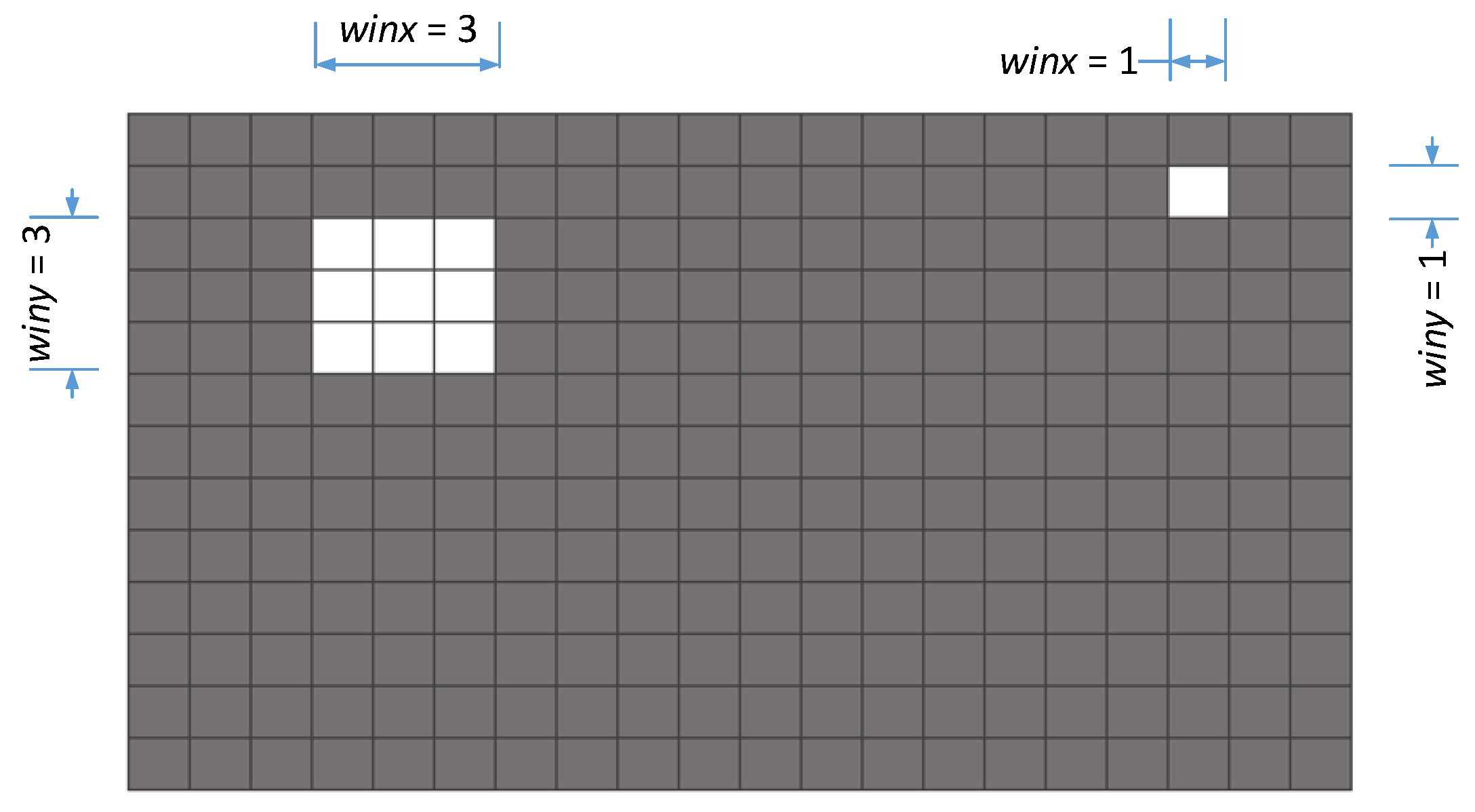
2.3. Adding and Removing Elements

The difference between SIMP and BESO is large when updating the design variables, where the former usually uses highly efficient algorithms like the optimality criteria (OC) methods or the method of moving asymptotes (MMA). A standard OC updating scheme is used in this paper, which can be formulated as [31]

$$x_e^{t+1}=\{\begin{array}{c}\max \left(x_{\text{min}}, x_e^t-m\right) \text{if} x_e^t{B}_e^{\eta }\le \text{max}\left(x_{\text{min}}, x_e^t-m\right)\hfill \\ \text{min}\left(1, x_e^t+m\right) \text{if} \text{min}\left(1, x_e^t+m\right)\le x_e^t{B}_e^{\eta }\hfill \\ x_e^t{B}_e^{\eta } \text{otherwise}\hfill \end{array},$$

(6)

where $x_e^t$ means the value of the design variable at iteration $t$, $\eta$ is a numerical damping coefficient (equal to 0.5 in this paper), $m$ is the positive move limit, and $B_e$ is given by the optimality condition as

$$B_e={\lambda }^{-1}p{x}_e^{p-1}{u}_e^{\mathrm{T}}{K}_e{u}_e,$$

(7)

in which $\lambda$ is a Lagrangian multiplier that can be determined using the bisection method.

As for BESO, in each iteration, the volume is evolved by

$$V_{t+1}=\max (V^{*}, V_t\left(1-ER\right))$$

(8)

where $ER$ means the evolutionary volume ratio. Another parameter called maximum volume addition ratio (AR) is usually used to guarantee that not too many elements are added in a single iteration, but it does not matter in our method, so we ignore it. The elements are removed according to their sensitivity numbers from low to high strictly until reaching the prescribed volume in this iteration, just like a kind of greedy heuristic search algorithm.

2.4. Convergence Criterion

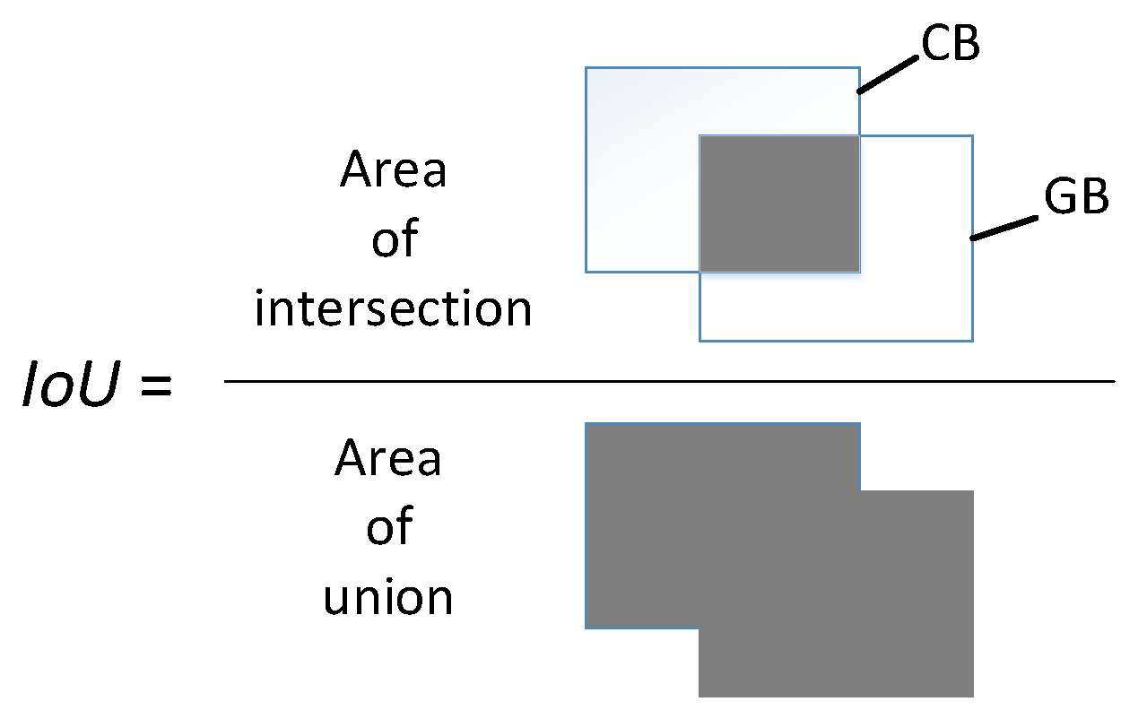
The convergence criterion is defined by the change of the objective function. After reaching the volume constraint $V^{*}$, the update process will not end unless the difference between the compliance in the past few iterations is little enough

$$\frac{\left|{{\displaystyle \sum }}_{i=1}^M\left(C_{t-i+1}-C_{t-M-i+1}\right)\right|}{{{\displaystyle \sum }}_{i=1}^M{C}_{t-i+1}}\le \tau ,$$

(9)

here, $M$ is an integral number, and $\tau$ is a little constant representing the convergence tolerance. Considering that the exploration will hamper the convergence, it will not be used when the volume of the topology decreases near the limited value.

2.5. Evaluation

To guarantee the engineering performance and the novelty of results, two metrics are calculated to evaluate the final structure in each episode:

First, the difference of performance (like compliance) between the current design and the reference design is considered. Those structures with low performance will be rejected.

Another metric named $IoU$ (intersection-over-union) is from a common evaluation metric for the object detection (Figure 1), which represents the similarity of the current structure and previous structures. It is calculated as the ratio of the intersection to the union of two rectangles called candidate bound $CB$ and ground truth bound $GB$

$$IoU=\frac{area\left(CB\right){{\displaystyle \cap }}^{}area\left(GB\right)}{area\left(CB\right){{\displaystyle \cup }}^{}area\left(GB\right)}.$$

(10)

Furthermore, $IoU$ can be extended to 3D flexibly if changing ‘area’ to ‘volume’.

3. Using Exploration Approaches of Reinforcement Learning in STO

The exploration–exploitation dilemma is a fundamental problem of reinforcement learning. Exploitation means making the best decision based on current information, while exploration indicates gathering more information, which helps make the best overall decision at the expense of efficiency.

Figure 2 shows how to combine those exploration approaches with STO briefly. ε-greedy helps disturb the search direction when adding and removing elements; UCB adds a bonus when calculating the sensitivity; TS and IDS replace sensitivity functions by posterior reward distributions and update the density of elements by sampling. Among them, UCB is used both in SIMP and BESO, while the remaining exploration strategies are only used in BESO because of their inconvenience in dealing with continuous variables. In this section, we describe the procedures in detail.

3.1. Naïve Exploration

In reinforcement learning, ε-greedy policy is a common method of exploration and mostly used for discrete action spaces. As in this book [8], ε-greedy policy is defined as

$$\pi (a|s)\leftarrow \{\begin{array}{c}1-\epsilon +\frac{\epsilon }{\left|A\left(s\right)\right|} \text{if} a=a^{*}\\ \frac{\epsilon }{\left|A\left(s\right)\right|} \text{if} a\ne a^{*}\end{array}$$

(11)

where $a^{*}$ denotes the best action for maximizing the predicted value, and $\left|A\left(s\right)\right|$ is the total number of actions in the state. By choosing an appropriate value of $\epsilon$, the balance between exploration and exploitation can be well achieved. In general, a decay schedule for $\epsilon$ is added as the algorithm running.

There are many variants of ε-greedy, one is called ‘greedy with optimistic’, which initializes the action-value function to high value, then almost every action will be tried theoretically, but it can still lock on to sub-optimal actions. Another is called ‘decaying ${\epsilon }_t$-greedy policy’, ${\epsilon }_t$ will decrease as the iteration and gap (difference in the value of the current action and the optimal action) increase. The regret of this method is lower, but advanced knowledge of gaps is required, which seems not realistic in practice. Moreover, there is another approach named Boltzmann exploration procedure based on thermology, using temperature to control the choice of actions, where the temperature is equivalent to $\epsilon$ in $\epsilon$-greedy.

In a word, exploration in these naïve exploration methods is achieved by randomization. While in BESO, elements are deleted based on the rank of sensitivity numbers completely like greedy algorithm. To use naïve exploration in BESO, a random perturbance during the process of adding and removing elements is needed. In order to prevent the whole structure from collapsing suddenly, we divide the elements into two classes based on the ranking of sensitivity numbers, which is inspired by the genetic algorithm used in BESO [2], the proportion of the higher class is $V^{*}/2$, and this mechanism is also used in all the other algorithms in Section 3. When deploying the $\epsilon$-greedy policy, after sorting the elements by their sensitivity numbers, the elements are divided into lower class and higher class, and the bottom (1 − ε) of the total elements which need deleting in this iteration are firstly removed as BESO, while the other ε portion are removed randomly from the lower class.

Moreover, $\epsilon$ is declined by iteration to make solutions convergent like the decaying $\epsilon$-greedy policy, the scheme is formed as

$$\epsilon \leftarrow {\epsilon }_0-{\epsilon }_0{\left(t/t_0\right)}^3,$$

(12)

in which ${\epsilon }_0$ means the value of $\epsilon$ at the beginning of the episode, and $t_0$ denotes the number of iteration when the volume fraction just reaching the minimum.

For some structures with detailed meshes, the effect of removing just one element is not obvious. Therefore, we use ‘search window’ (Figure 3) when removing the elements, which means deleting one element as well as its neighbors at the same time. The size of the search window is controlled by two parameters: $winx,winy$, and it can be expanded to 3D cases easily.

3.2. Optimistic Exploration

Optimistic exploration means those uncertain actions are more likely to be chosen. To measure the uncertainty, the frequency of each action is calculated as an additive term, namely bonus when choosing actions

$$A_t=\underset{a}{\mathrm{argmax}} [Q_t\left(a\right)+cB\left(a\right)],$$

(13)

in which $Q_t$ is the action-value function, and $c$ is a positive parameter that controls the degree of exploration, a bigger $c$ means more exploration.

Upper confidence bound, or UCB [26,27], is the most popular algorithm for this kind, where the bonus is

$$B\left(a\right)=\sqrt{\frac{2\ln t}{N\left(a\right)}},$$

(14)

in which $N\left(a\right)$ is the number of times the action $a$ has been selected, and $t$ means the number of iterations. There are also some variants of UCB, but the main difference between those methods and greedy exploration is the bonus, no matter what the bonus is. In a word, the key point of optimistic exploration is keeping the balance between the uncertainty and optimality.

In STO, the idea of UCB is adopted in the process of calculating the sensitivity

$${\alpha }_t^e={\alpha }_t^e-c\sqrt{\frac{ln\left(t\right)}{2N\left(a_t^e\right)}},$$

(15)

where $N\left(a_0^e\right)=1$ in the beginning. In SIMP, $N\left(a\right)$ is calculated as the increment of the density

$$N\left(a_{t+1}^e\right)=N\left(a_t^e\right)+\max \left(0,x_{t+1}^e-x_t^e\right),$$

(16)

As for BESO, because the initial elements are all solid and their density is discrete, $N\left(a\right)$ is updated by their times of keeping solid states

$$N\left(a_{t+1}^e\right)=N\left(a_t^e\right)+1 if x_{t+1}^e=1$$

(17)

In this way, these elements with low probability to be removed are more likely to be deleted now, and the probability will increase as the value of $c$ increases. Normally, $c$ should be chosen to make the magnitude of sensitivity and bonus similar.

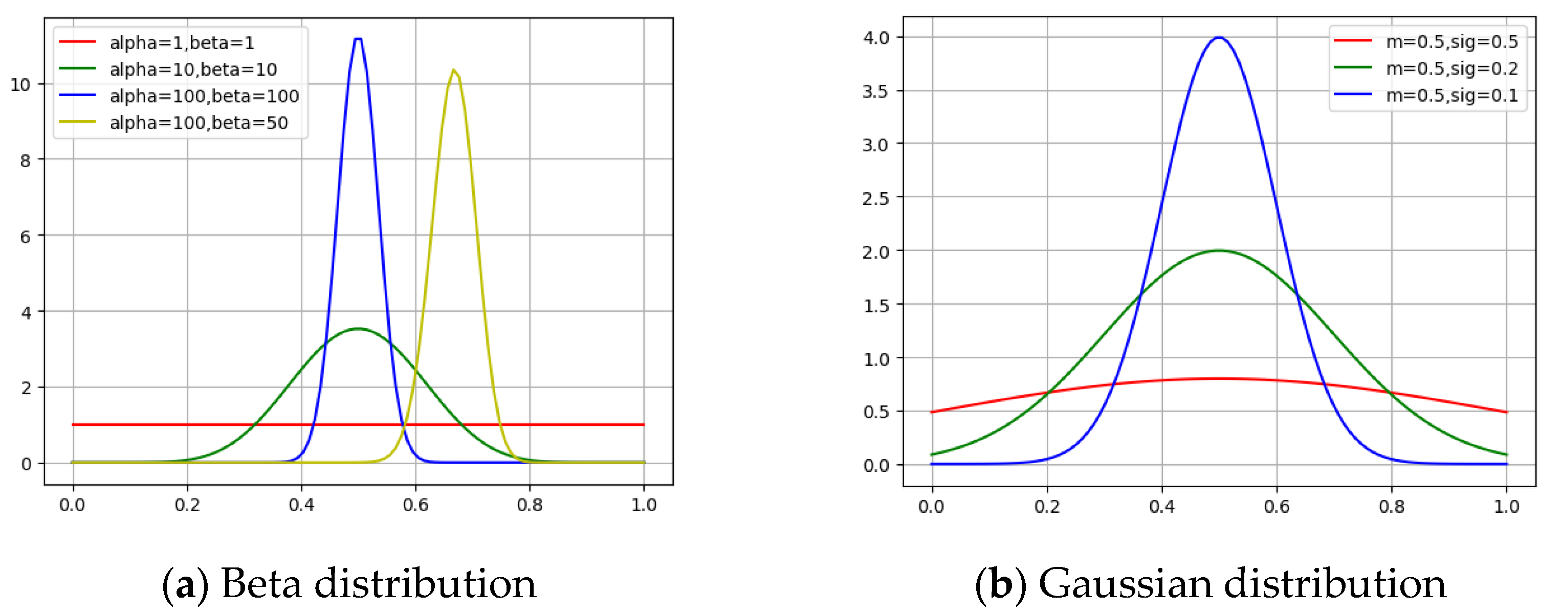
3.3. Probability Matching

Probability matching, also called posterior sampling, uses posterior probability to achieve exploration based on Bayesian theory, whose idea is also to encourage the exploration of uncertain actions. This scheme is also called Thompson Sampling [28], which chooses each action according to its probability of being optimal

$$\pi \left(a|h_t\right)=P\left[Q\left(a\right)>Q\left(a^{\prime }\right), \forall a^{\prime }\ne a|h_t\right]=E_{R|h_t}[1(a=\underset{a\in A}{\mathrm{argmax}}Q\left(a\right))]$$

(18)

where $h_t$ is the history sequence of action and reward, $\pi \left(a|h_t\right)$ means the probability to choose action $a$ under $h_t$, $Q\left(a\right)$ represents the action-value function and $R$ means reward function. The brief steps of Thompson sampling are below:

• Sample the reward $R$ from the posterior reward distribution $P$
• Compute the action-value function $Q\left(a\right)=\mathrm{E}\left[R_a\right]$
• Take the optimal action by Equation (18)
• Execute the chosen action in actual environment and get the reward $r_t$
• Update the posterior distribution $P$ by Equations (19) and (20)

As the learning process going on, the confidence interval of each action will be narrower and narrower towards convergence.

In BESO, like exploring the multi-armed bandit problems, elements are just like the arms of the bandit, and those exploration methods help decide which arm to be chosen (deleted). Reward is defined as the rank of the sensitivity numbers of elements, 0 to 1 from higher sensitivity to lower sensitivity, then elements with higher reward (lower sensitivity) are more likely to be chosen (removed). The actual reward distribution of each action is gained by previous ranks. To describe the reward distribution, there are two frequently used patterns named Beta distribution and Gaussian distribution shown in Figure 4. Beta distribution is a kind of binomial distribution with two parameters Beta($\alpha , \beta$). Despite its proofs are a bit complex, its update scheme is simple and can describe the sampling process well, which is

$$(\alpha , \beta )=(\alpha , \beta )+(r_t, 1-r_t)$$

(19)

For example, the initial distribution is Beta($1,1$) without any prior knowledge, each action has the same reward. Then $\alpha$ and $\beta$ increase as the number of sampling increases. As a result, the distribution function will be narrower and narrower near the mean value.

Gaussian distribution also has two parameters N($\mu , {\sigma }^2$), which are updated by

$$\begin{gathered} {\mu }_{t+1, a}=\left(\frac{{\mu }_{t, a}}{{\sigma }_{t,a}^2}+\frac{Y_{t, a}}{{\sigma }_0^2} \right)/(\frac{1}{{\sigma }_{t,a}^2}+\frac{1}{{\sigma }_0^2}) \\ {\sigma }_{t+1, a}={\left(\frac{1}{{\sigma }_{t,a}^2}+\frac{1}{{\sigma }_0^2}\right)}^{-1} \end{gathered}$$

(20)

in which $Y_t$ is the observation drawn independently from the actual reward distribution N(${\mu }_0, {\sigma }_0^2$). The variance ${\sigma }^2$ will decrease as the number of sampling increases, then the distribution function will more and more concentrate on the mean value $\mu$.

3.4. Information State Search

Information state search views information as a part of state. The idea of this kind of method is choosing the action with the most information gain. The most representative approach is called information-directed search (IDS) [29], in which action is sampled by minimizing the ratio of squared expected single-period regret and information gain

$$a=\underset{a}{\mathrm{argmin}}\frac{\mathsf{\Delta }{\left(a\right)}^2}{g\left(a\right)}$$

(21)

where $\mathsf{\Delta }\left(a\right)=E\left[r\left(a^{*}\right)-r\left(a\right)\right)]$ represents the difference of the rewards earned by the optimal action and the actual action, $g\left(a\right)$ is the information gain of $a$ and equal to the expected reduction in the entropy $H$ of ${\gamma }_t$ due to the observation, ${\gamma }_t$ means the posterior distribution of $A^{*}$:

$$\begin{gathered} g_t\left(a\right)=E[H\left({\gamma }_t\right)-H\left({\gamma }_{t+1}\right)|h_t, A_t=a] \\ {\gamma }_t\left(a\right)=P(A^{*}=a|h_t) \end{gathered}$$

(22)

To calculate $\mathsf{\Delta }$ and $g$, some approximated methods must be utilized, because the integrals in posterior distribution should be computed over high-dimensional spaces. First, near-exact approximations can be gained by calculating integrands at discrete gird of points. Another attempt is replacing integrals with sample-based estimates, which reduces the time complexity especially when calculating the integration over high-dimensional spaces. We prefer the latter method in this paper. The brief steps are below:

• Get the samples for estimation by interacting with the actual environment in the first iteration, and by the updated posterior reward distribution $P$ in the following steps
• Compute $\mathsf{\Delta }$, $g$ and the information gain ratio
• Take the optimal action by Equation (21)
• Execute the chosen action in actual environment and get the reward
• Update the posterior reward distribution by Equations (19) and (20)

In BESO, the definition of the reward is the same as that in Section 3.3, but the number of actions must be down because of its high time complexity. Thus, we proceed the STO by BESO in the first episode, then divide the elements by the rank of sensitivity numbers into 10 to 20 groups, and each group is corresponding to one action which can be chosen (deleted) for a certain times equal to the number of solid element it contains. In the following episodes, the number of elements that need deleting in each group will be allocated by IDS first, after that, the elements in each group are chosen by sampling according to the actual reward function of each element.

4. Cases and Discussion

This section applies different exploration methods above combining with SIMP and BESO to several well-known 2D and 3D minimum compliance problems, and then filters these final structures by evaluation. After that, a bunch of design options and stacked views are generated, and the degree of variation can be controlled by one parameter for each method simply, when improving $\epsilon$ of ε-greedy policy, $c$ of UCB, as well as the variance of the posterior distribution of TS and IDS, more novel structures will be created, but at higher risk of divergence.

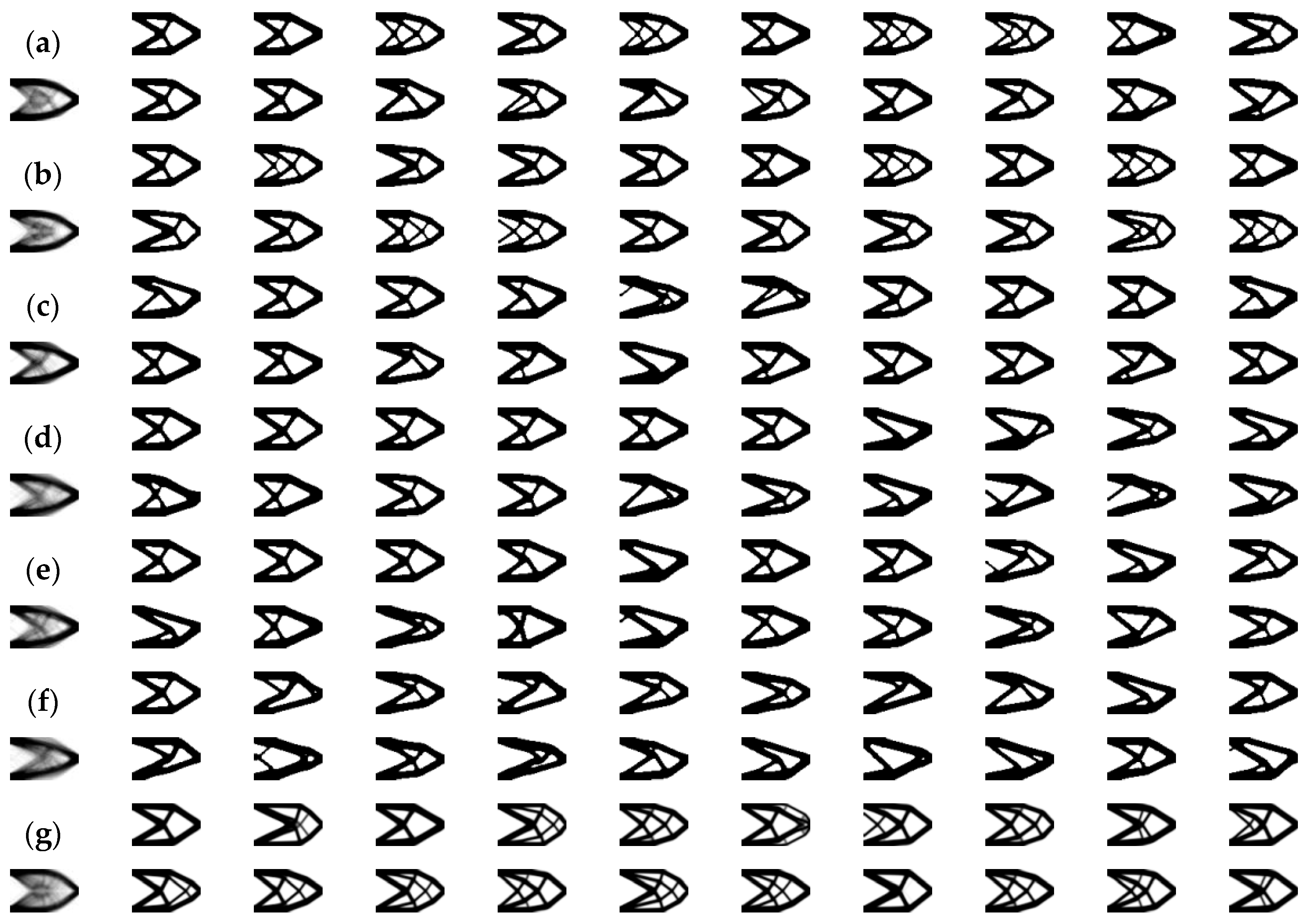
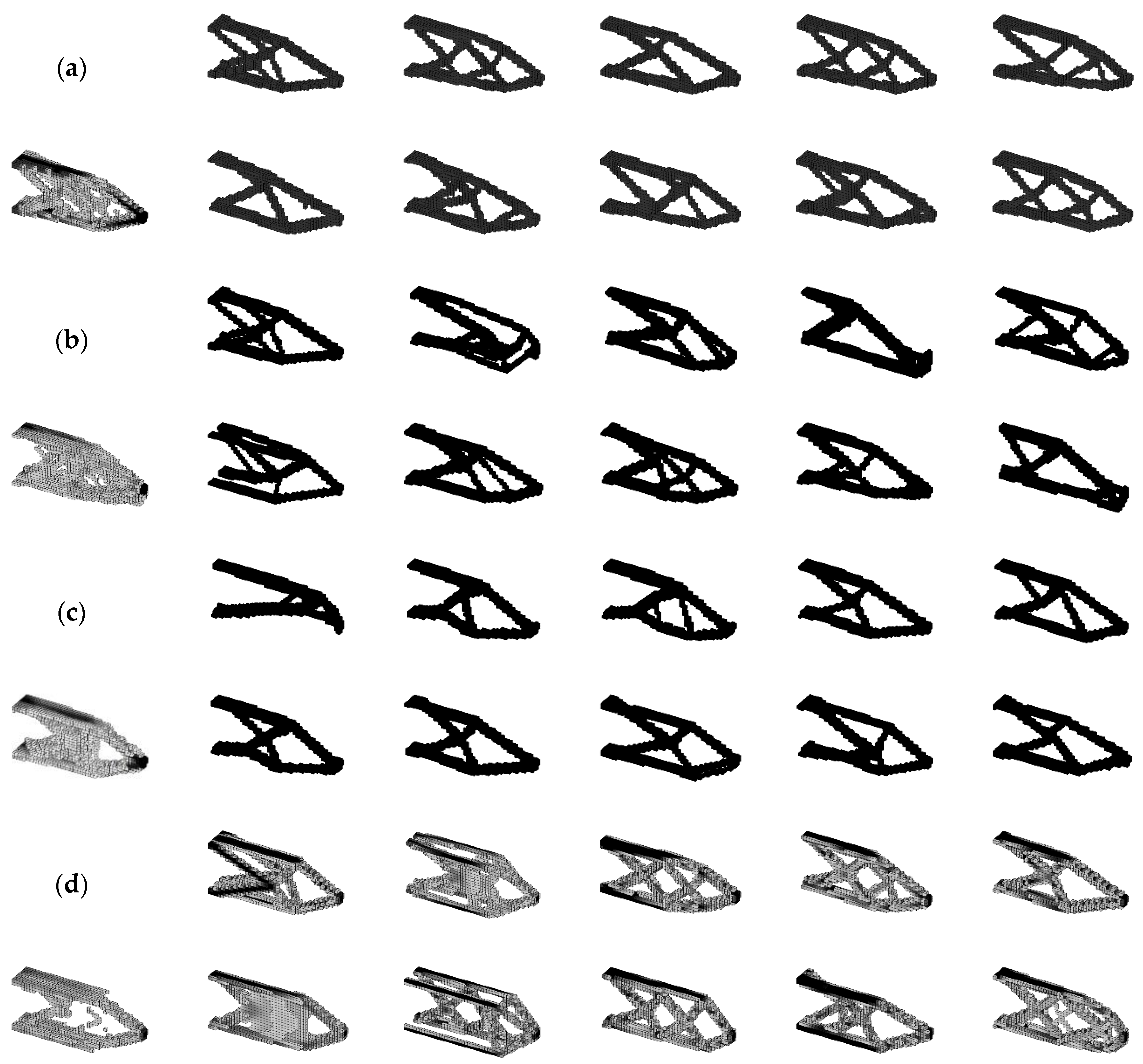
4.1. Cantilever Beam

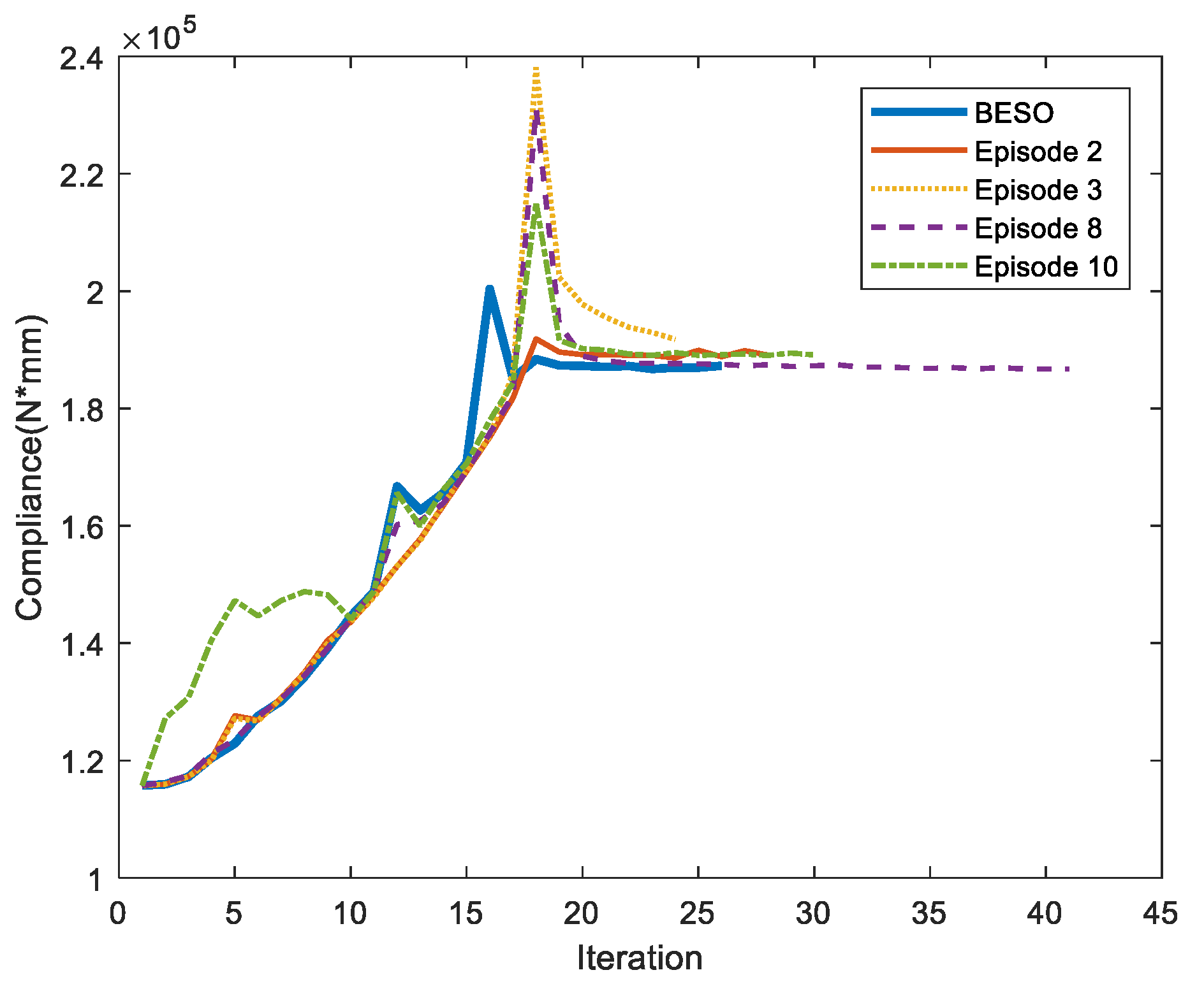
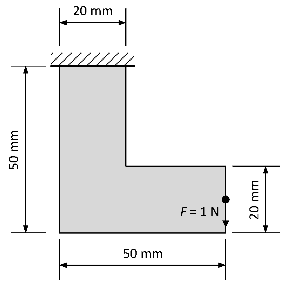
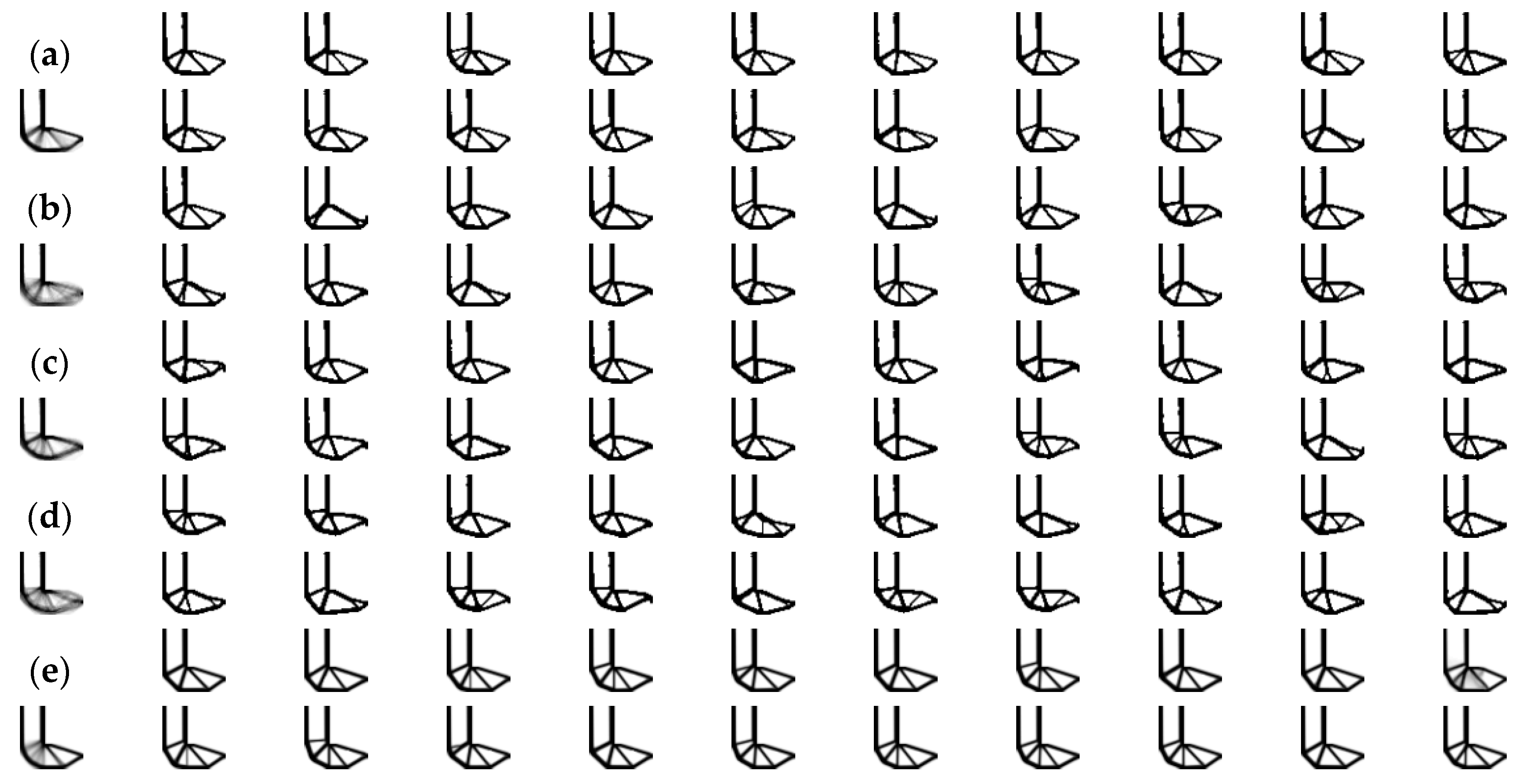
A 2D cantilever beam is given to demonstrate the performance of different exploration algorithms. Figure 5 shows the design domain of the structure with its load and boundary conditions. Young’s modulus $E=1\mathrm{MPa}$ and Poisson’s ratio $\mathsf{\upsilon }=0.3$ are assumed. The objective volume fraction is set to 50% of the total area of the design domain. Other BESO parameters are shown below: the evolution volume ratio $ER=0.04$, the filter radius $r_{min}=4\mathrm{mm}$, the minimum design variable $x_{\min }=0.001$, $M=5,$ $\tau =0.1$% for the convergence criterion and the penalty exponent $p=3.0$. Parameters of SIMP are $m=0.2$, $r_{min}=4\mathrm{mm}$, and $\tau =1$%. Moreover, the evaluation standards are those designs whose compliance is below twice of that of the benchmark structure and whose $IoU$ is below 0.9.

First, the decaying $\epsilon$-greedy policy is used. The first result is calculated by BESO, and the rest are got by setting $\epsilon =0.05$ or $\epsilon =0.1$ with $winx=winy=3$. By the way, it is worth mentioning that the structures tend to be asymmetric. Therefore, to keep the diversity, the symmetry constraint is added for getting some symmetric results.

Second, UCB algorithm is applied with BESO. Four results satisfying the demand are got when $c=1$ in 10 episodes, and the rest 16 results are generated by varying $c$ from 1 to 1000.

Third, TS is utilized based on two distributions. The diversity of the topologies can be controlled by zooming the variance of the posterior distribution of reward. For beta distribution, diverse final topologies can be gained from varying the increment of $\alpha \mathrm{and} \beta$ from 0.1* to 10*. For gaussian distribution, diverse final topologies can be gained by varying $\sigma$ of the model from 1* to 100*.

Fourth, IDS is also used on two distributions. The rate for beta distribution varies from 0.1 to 10, and the rate for gaussian distribution varies from 1 to 100.

Finally, UCB is combined with SIMP, and the range of $c$ is from 0.05 to 0.1 to get the designs.

All topologies are shown in Figure 6, we can see that all the seven methods can generate diverse acceptable structures successfully. UCB can keep the symmetry of origin structure, while $\epsilon$-greedy policy cannot keep the symmetry of structures without the symmetry constraint, the results of TS and IDS can be symmetric randomly. Furthermore, IDS needs more computation resource. The good phenomenon is that UCB, TS, and IDS usually generate divergent structures in the first one or two episodes because of the exploration, but after that the quality of the structures is improved as the shrink of the search space. As for the difference of SIMP and BESO, the former sometimes generates intermediate densities (gray elements), which make the solutions unable to be adopted directly.

To enable a clear visualization of the exploration process, we also show a stacked mode for all results in Figure 6. With this view, users can see discrepancies as well as common features in different topologies directly. The color for each pixel is easy to get by calculating the average color at that pixel for all individual designs, so the stacked view is equal to the average of generative designs. In those stacked views, the importance of different parts is shown obviously, we can see that the main frame is invariant for those designs, while the inner microstructures always change.

The details of the design by UCB with BESO are presented as an example. The information about compliance, $IoU$ and iterations of the design in each episode is listed in

Table 1. Calculation results of the cantilever beam by UCB with BESO.

Nth Episode	$\mathit{C}({10}^5 \mathrm{N}·\mathrm{mm})$	IOU	ITER	Nth Episode	$\mathit{C}({10}^5 \mathrm{N}·\mathrm{mm})$	IOU	ITER
BESO	1.873		26	11	1.923	0.736	43
2	1.891	0.600	28	12	1.878	0.851	34
3	1.918	0.779	24	13	1.873	0.740	46
4	1.885	0.794	55	14	1.912	0.801	34
5	1.883	0.856	24	15	1.876	0.896	29
6	1.883	0.695	37	16	1.881	0.858	26
7	1.877	0.746	31	17	1.913	0.866	75
8	1.867	0.859	41	18	1.900	0.894	42
9	1.878	0.870	28	19	1.963	0.719	100
10	1.891	0.868	30	20	1.886	0.893	40

. The compliance and $IoU$ of all topologies satisfy evaluative criteria, which means that enough engineering performance and diversity of the designs can be guarantee. Furthermore, the numbers of iterations of most episodes are similar to that of BESO, meaning that the computation cost is acceptable. The evolutionary histories of the objection function of five episodes are shown in Figure 7. The curves are usually not monotonous with one or more peaks, and the corresponding iteration and the amplitude of peaks are different in different episodes, representing various search directions.

4.2. L-Shaped Beam

In the second example, we demonstrate the design problem for a L-shaped beam sketched in Figure 8, which is loaded at the center of the rightmost free end by $F=-1\mathrm{N}$. The beam is discretized into 1600 quadrilateral elements with 40% maximum volume fraction. Material properties are $E=1\mathrm{MPa}$ and $\mathsf{\upsilon }=0.3$. The parameters of BESO are set to $ER=0.03$, $r_{min}=2\mathrm{mm}$, $x_{\min }=0.001$,$M=5,$ $\tau =1$%, and $p=3.0$. SIMP parameters are $m=0.2$, $r_{min}=1.5\mathrm{mm}$, and $\tau =0.01$%. Evaluation standards are the same as those in Section 4.1.

The parameters of the exploration approaches are below: first, $\epsilon =0.05$, 0.10, and 0.15 with $winx=winy=1$ is used for $\epsilon$-greedy policy. Then, in UCB, $c=1,10,\mathrm{and}100$ for BESO, and $c=0.3 \mathrm{to} 10$ for SIMP. As for TS and IDS, we test 0.1* to 10* for beta distribution, and 1* to 100* for gaussian distribution.

Figure 9 shows all the final topologies generated by five methods except IDS, because IDS almost always creates divergent results for this case, the reasons may be the fragile structure around the corner and the low filter radius make the structure more likely to be disconnected. Results of other methods seem no problems, what is not perfect is that some results has mall holes, it does not matter as the number of results increases, or the problem can be solved by rising the filter radius.

From the stacked views in Figure 9, we can see that there is a same clear main frame for structures of each method, and the changeable parts concentrate on the bottom.

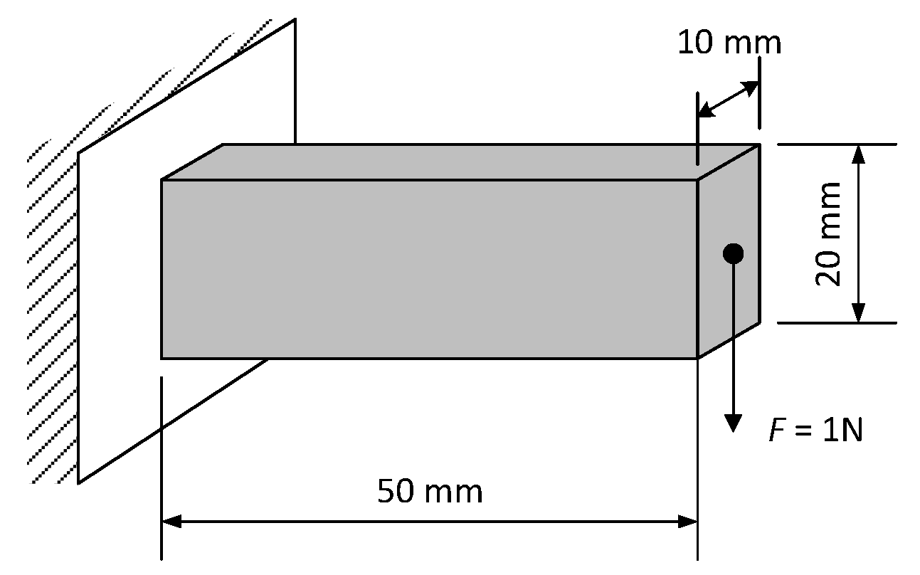
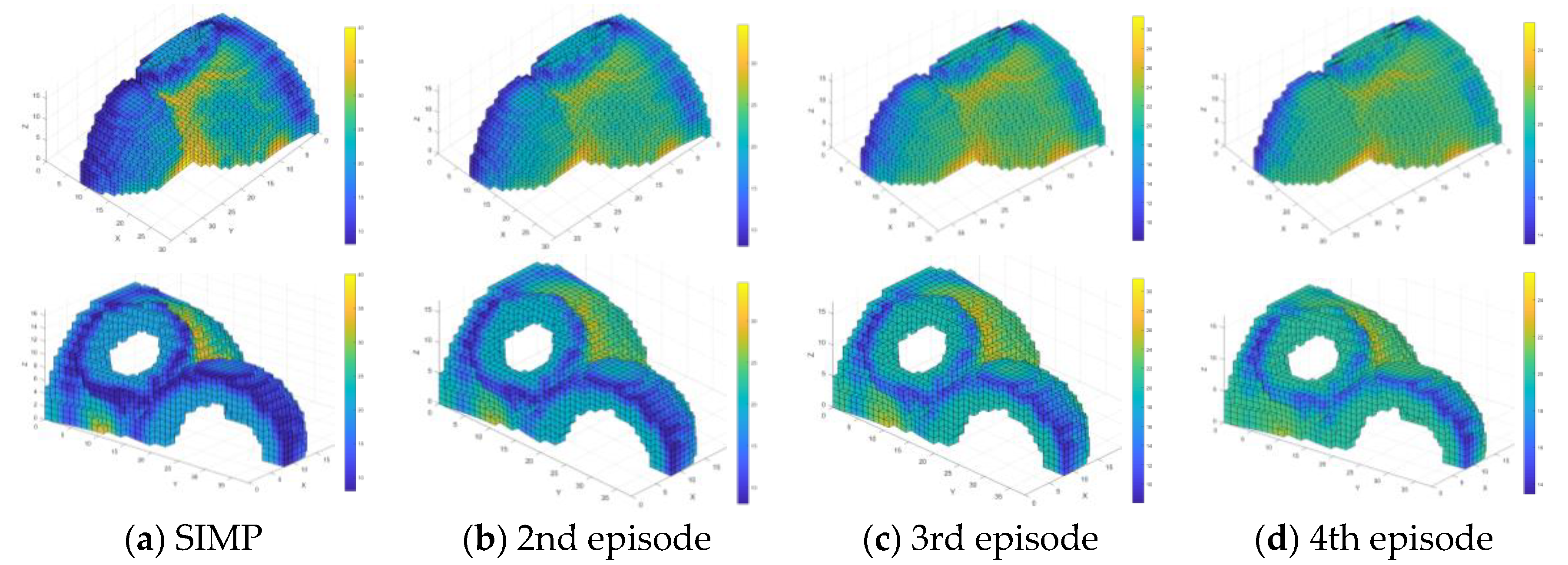
4.3. 3D Cantilever Beam

Those proposed exploration approaches can be extended to three dimensions straightforwardly, a STO problem for a 3D cantilever beam is shown in Figure 10. The design domain is $50\times 20\times 10\mathrm{mm}$ in shape and discretized using 10,000 eight node cubic elements. Only 10% volume of the design domain is available. The material has $E=1\mathrm{MPa}$ and $\mathsf{\upsilon }=0.3$. BESO parameters $ER=0.03$, $r_{min}=1.5\mathrm{mm}$, $x_{\min }=0.001$, $M=5,$ $\tau =1$%, and $p=3.0$ are used. SIMP parameters are $m=0.2$, $r_{min}=1.5\mathrm{mm}$, and $\tau =1$%. The evaluation for compliance is the same as above but the maximum $IOU$ is set to 0.7, because $IOU$ of the generated designs is usually lower in 3D cases.

Due to the time consuming nature of complex 3D cases, only 10 designs are shown for each method in Figure 11, and beta distribution need not be considered because it has shown the same effect as gaussian distribution. Four exploration methods are used, $\epsilon$-greedy policy with $\epsilon =0.10$ and $winx=winy=winz=1$, UCB with $c=1\mathrm{to}10$ for both BESO and SIMP as well as TS with 1* and 10* increment for beta distribution are chosen, Diverse design options are generated successfully. As shown in Figure 11d, the phenomenon of gray elements is more severe for the case with low volume fraction, but the good thing is SIMP needs less computation time than BESO. Results by IDS are below our expectation, which are always divergent, the reason is that IDS tends to disconnect the structure easily under small volume constraints.

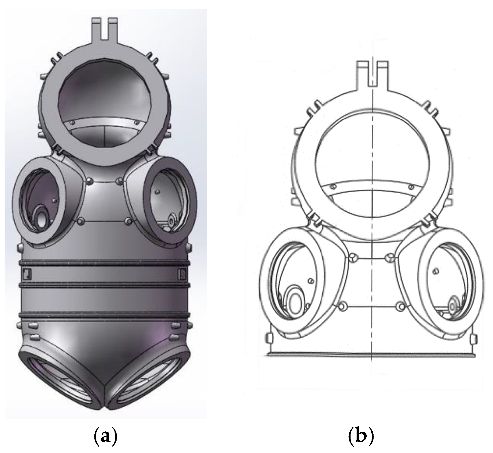
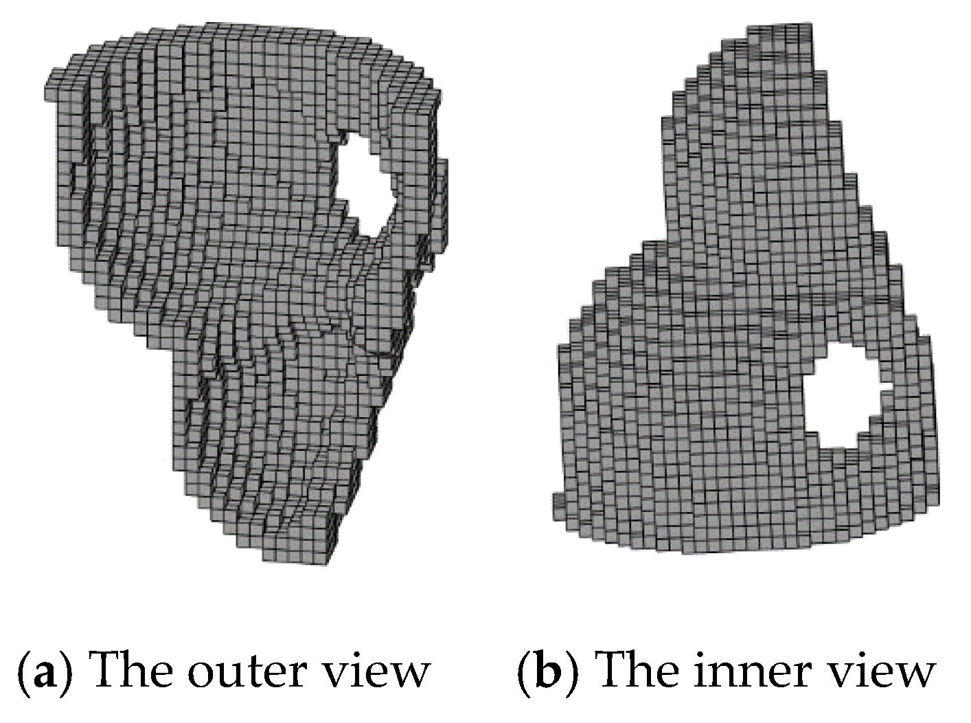
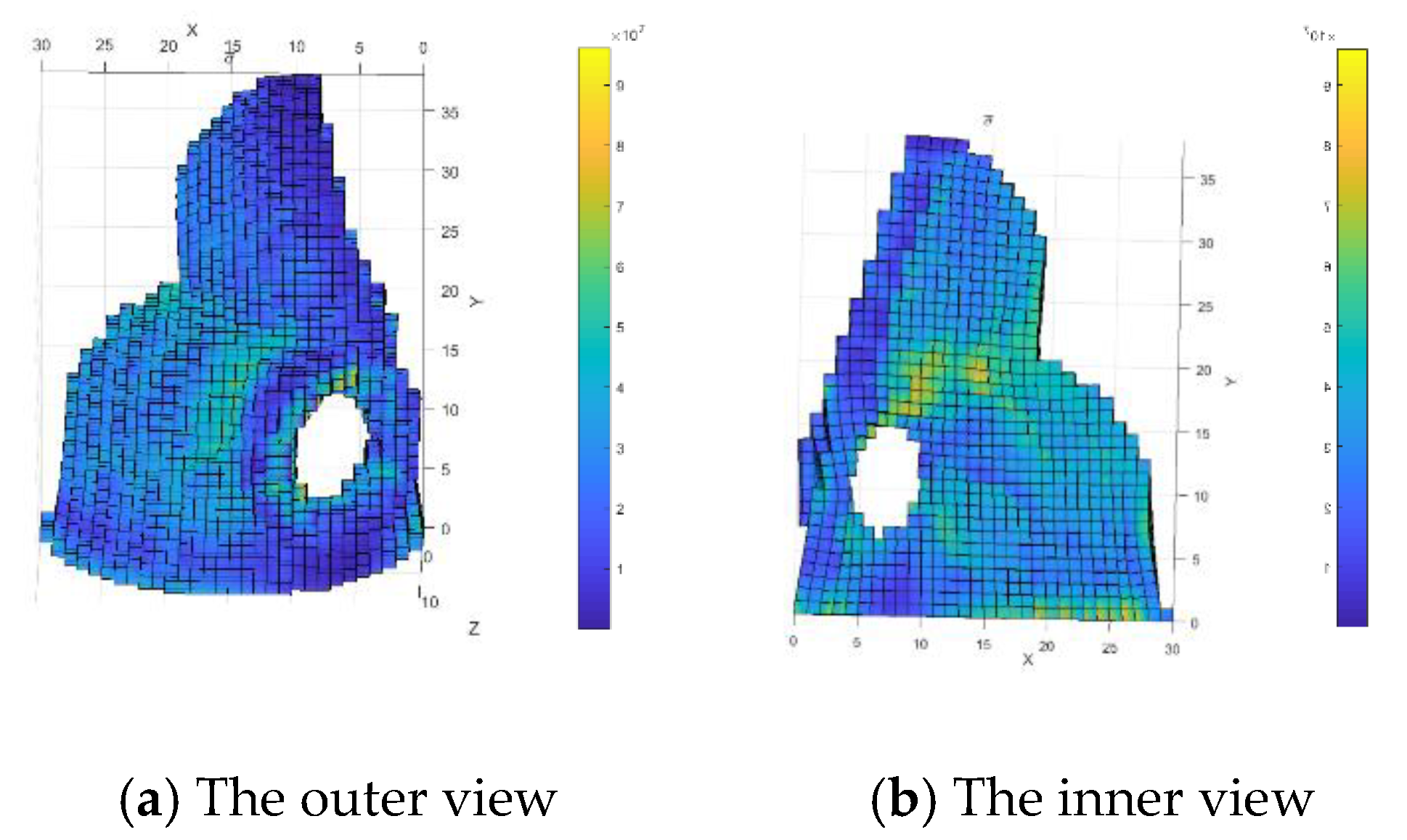
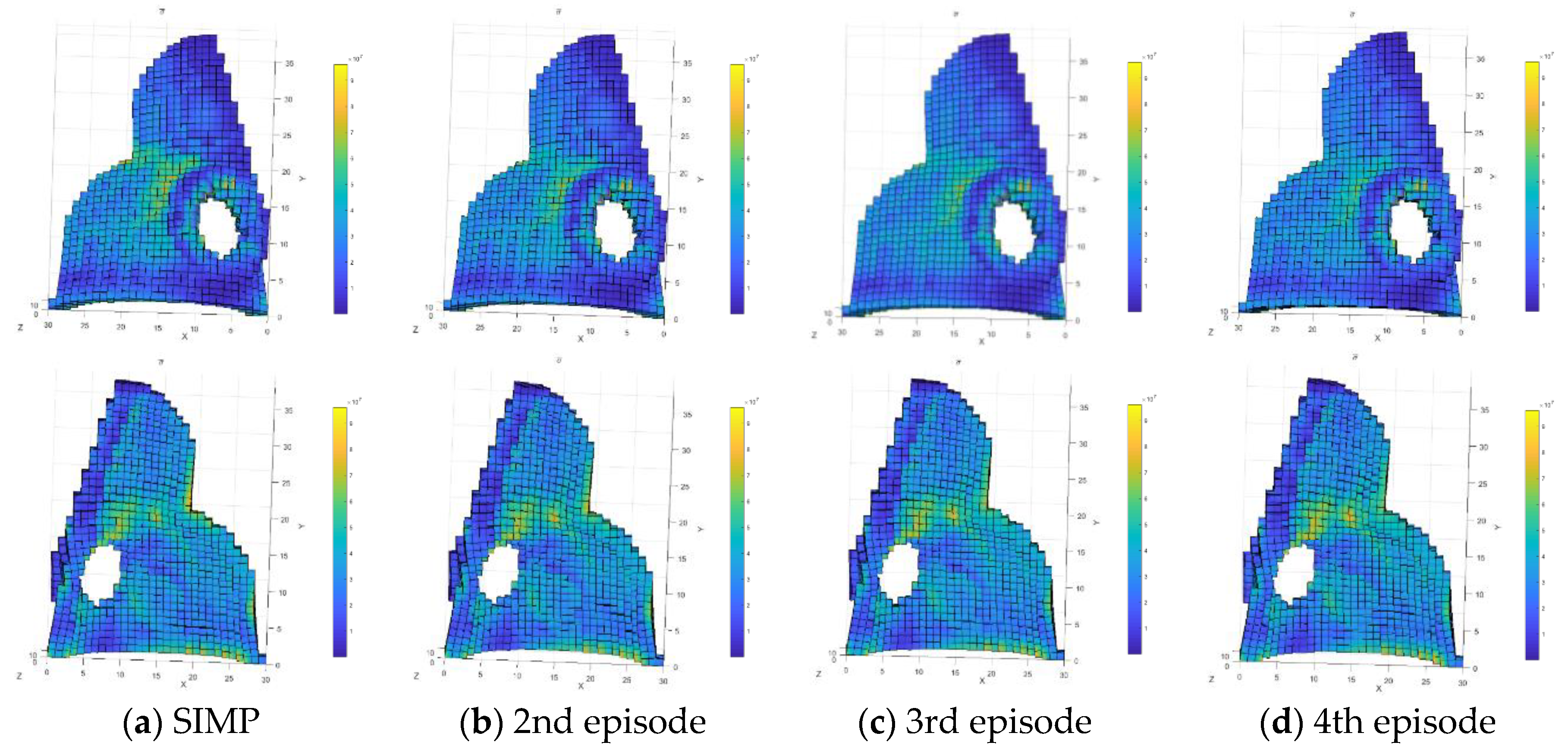
4.4. Upper Body of an Atmospheric Diving Suit

The final case is based on a practical engineering problem of China Ship Scientific Research Center, which is the design of an atmospheric diving suit (ADS), seen in Figure 12a. We chose its upper body as an example to test our exploration algorithm. To simplify the problem, stability, gravity, hydrodynamics, and the minor parts—such as holes or lugs—are not considered.

The main dimensions are shown in Figure 12b, and the structure is set to be fixed on the connections of head, arms, and the lower part. The maximum working depth is 500 m and the calculation pressure is set to 9 Mpa after considering the safety. Material properties are $E=68.9\mathrm{Gpa}$, $\mathsf{\upsilon }=0.3$, and the allowable stress is 208 Mpa.

Because the thickness is much lower than the size of the shape, the size of the structure must be large enough to guarantee enough elements to be deleted, which needs huge computation source. To avoid this problem, we transferred it to a variable thickness design problem, which means changing the density of elements on the outer surface instead of removing them, it can be simply achieved by setting $p=1$ in SIMP, then the thickness can be represented by density. The goal is optimizing the distribution of thickness without changing the weight.

Because the code is written in MATLAB, the geometric model should be imported from Solidworks first as shown in Figure 13. The upper body is discretized using 8-node hexahedral element, whose size is $20\times 20\times 20\mathrm{mm}$. The density of elements are all initialized to 0.5 and varying between 0.2 and 1, which means the thickness of outer elements varies between 8 and $40\mathrm{mm}$. In order to avoid the case that the thickness declines to 0 in some region, which may cause the structural failure by leakage or corrosion, the minimum thickness is set to $40\times 0.2=8\mathrm{mm}$. Figure 14 shows the stress contour of the origin structure, the value of stress is higher near the inner surface of neck as well as the connections of body and arms. The maximum stress is 96.1Mpa, and the total compliance is 230.2$\mathrm{N}·\mathrm{m}$.

The design domain is only the outer surface (not including the connected parts). SIMP parameters are $m=0.2,p=1,r_{min}=40\mathrm{mm},M=3,\tau =1$%. The evaluation for compliance is the same as above but maximum $IOU$ is set to 0.95 because the space of optimization is limited for this case, in addition, the maximum element stress is also a metric of evaluation, which cannot exceed the allowable stress.

UCB with $c=30,000$ is used to generate four topologies (Figure 15), whose information is shown in

Table 2. Calculation results of the upper body of ADS.

Nth Episode	$\mathbf{C}(\mathbf{N}·\mathbf{m})$	$\mathbf{\Delta }\mathit{C}$	IOU	Maximum Stress (Mpa)	ITER
SIMP	214.9	---	---	96.3	7
2	218.6	1.7%	0.860	96.1	9
3	220.9	2.8%	0.940	96.0	9
4	226.4	5.3%	0.936	95.9	6

and contour distribution can be seen in Figure 16. According to the first design calculated by SIMP, the material accumulates around the neck, back and chest, meaning these parts need to be thickened. And from Figure 16a–d, more uniform the thickness is, higher compliance the structure has. In addition, the maximum and distribution of stress are almost invariant, which means our proposed method can decrease the compliance by controlling the thickness distribution without changing the weight and stress distribution of the structure.

The stress calculated by our code in MATLAB is not highly precise, because the size of the element is large and the hexahedral elements can’t fit the curved surface very well. Thus, the results focus more on providing guidance for designers during the conceptual design.

5. Conclusions and Future

In this paper, we focus on adding the features of the exploration approaches in reinforcement learning to the procedures of SIMP and BESO, so as to increase the search ability of structural topology optimization methods to generate multiple solutions. Then, the capability of those combined methods is demonstrated on three minimum compliance STO problems, including 2D and 3D cases, and the degree of exploration can be controlled with one parameter easily. The source code can be found at https://github.com/Nick0095/STO_exploration.

By comparison, $\epsilon$-greedy policy with random search is easy to deploy, but to get satisfying designs, additional schemes are necessary sometimes, such as the search window for dense mesh and the symmetric constraint for symmetric structures. UCB is used as a bonus when calculating the sensitivity numbers, which encourages exploration of less-exploited elements, and it is able to create acceptable results without adding the computation complexity dramatically. TS is a method based on Bayesian theory and needs a little more computation resource, it estimates the value of elements by updating the posterior probabilities, which is more accurate compared with random search and heuristic rules. Finally, IDS is a new information-directed sampling method, but limited in its high demand for computing capacity. When dealing with STO problems, an approximation step is added to decrease the number of design variables, which maybe hampers its performance. In our cases, it can work for the simple cantilever beam, but the divergence always occurs when facing more complex structures. We believe it has potential as the computation ability increases in the future. Furthermore, beta distribution as well as gaussian distribution have similar functions and both work well in describing the posterior reward distribution of elements.

As for SIMP and BESO, although the solving algorithm of BESO is not so precise, it is not a big problem for generative design, and the discrete variables make it easier to be combined with various exploration approaches. SIMP can be solved by more efficient algorithms, but the gray problem cannot be neglected for designs with low volume fraction, on the other hand, that makes SIMP suitable for variable thickness design problems.

Low efficiency is still the bottleneck of the development of reinforcement learning, a highly efficient exploration approach that keeps the balance of searching ability and computation complexity is needed. According to the trend of development in RL, more and more experience can be referred to deal with large-scale combinatorial optimization problems like structural topology optimization. Furthermore, the compliance minimization problem is only a basic problem to test our proposed method, after that, we will try it in more kinds of problems with different objection functions and constraints, so as to make it more widely used. Also, achieving these algorithm in those commercial softwares with more kinds of elements is another choice to improve the efficiency and accuracy.

References

1. Liu, X.; Yi, W.J.; Li, Q.S.; Shen, P.S. Genetic evolutionary structural optimization. J. Constr. Steel Res. 2008, 64, 305–311. [Google Scholar] [CrossRef]
2. Zuo, Z.H.; Xie, Y.M.; Huang, X. Combining genetic algorithms with BESO for topology optimization. Struct. Multidiscip. Optim. 2009, 38, 511–523. [Google Scholar] [CrossRef]
3. Kaveh, A.; Hassani, B.; Shojaee, S.; Tavakkoli, S.M. Structural topology optimization using ant colony methodology. Eng. Struct. 2008, 30, 2559–2565. [Google Scholar] [CrossRef]
4. Luh, G.C.; Lin, C.Y. Structural topology optimization using ant colony optimization algorithm. Appl. Soft Comput. 2009, 9, 1343–1353. [Google Scholar] [CrossRef]
5. Luh, G.C.; Lin, C.Y.; Lin, Y.S. A binary particle swarm optimization for continuum structural topology optimization. Appl. Soft Comput. 2011, 11, 2833–2844. [Google Scholar] [CrossRef]
6. Aulig, N.; Olhofer, M. Topology optimization by predicting sensitivities based on local state features. In Proceedings of the 5th European Conference on Computational Mechanics (ECCM V), Barcelona, Spain, 20–25 July 2014. [Google Scholar]
7. Nikola, A.; Olhofer, M. Neuro-evolutionary topology optimization of structures by utilizing local state features. In Proceedings of the 2014 Annual Conference on Genetic and Evolutionary Computation, Vancouver, BC, Canada, 12–16 July 2014; pp. 967–974. [Google Scholar]
8. Sutton, R.S.; Barto, A.G. Reinforcement Learning: An Introduction, 2nd ed.; MIT Press: Cambridge, MA, USA, 2018; pp. 19–114. [Google Scholar]
9. Shea, K.; Aish, R.; Gourtovaia, M. Towards integrated performance-driven generative design tools. Automat. Constr. 2005, 14, 253–264. [Google Scholar] [CrossRef]
10. Krish, S. A practical generative design method. Comput. Aided Design. 2011, 43, 88–100. [Google Scholar] [CrossRef]
11. Kang, N. Multidomain Demand Modeling in Design for Market Systems. Ph.D. Thesis, University of Michigan, Ann Arbor, MI, USA, 2014. [Google Scholar]
12. Autodesk, Generative Design. Available online: https://www.autodesk.com/solutions/generative-design (accessed on 1 January 2019).
13. McKnight, M. Generative Design: What it is? How is it being used? Why it’s a game changer. KNE Eng. 2017, 2, 176–181. [Google Scholar] [CrossRef] [Green Version]
14. Justin, M.; Glueck, M.; Bradner, E.; Hashemi, A.; Grossman, T.; Fitzmaurice, G. Dream lens: Exploration and visualization of large-scale generative design datasets. In Proceedings of the 2018 CHI Conference on Human Factors in Computing Systems, Montreal, QC, Canada, 21–26 April 2018; p. 369. [Google Scholar]
15. Sosnovik, I.; Oseledets, I. Neural networks for topology optimization. Russ. J. Numer. Anal. Math. 2019, 34, 215–223. [Google Scholar] [CrossRef] [Green Version]
16. Rawat, S.; Shen, M.H. Application of Adversarial Networks for 3D Structural Topology Optimization. SAE Tech. Pap. 2019. [Google Scholar] [CrossRef]
17. Yu, Y.; Hur, T.; Jung, J.; Jang, I.G. Deep learning for determining a near-optimal topological design without any iteration. Struct. Multidiscip. Optim. 2019, 59, 787–799. [Google Scholar] [CrossRef] [Green Version]
18. Oh, S.; Jung, Y.; Kim, S.; Lee, I.; Kang, N. Deep generative design: Integration of topology optimization and generative models. J. Mech. Design. 2019, 141, 111405. [Google Scholar] [CrossRef] [Green Version]
19. Bendsøe, M.P. Optimal shape design as a material distribution problem. Struct. Optim. 1989, 1, 193–202. [Google Scholar] [CrossRef]
20. Young, V.; Querin, O.M.; Steven, G.P.; Xie, Y.M. 3D and multiple load case bi-directional evolutionary structural optimization (BESO). Struct. Optim. 1999, 18, 183–192. [Google Scholar] [CrossRef]
21. Huang, X.; Xie, Y.M. Convergent and mesh-independent solutions for the bi-directional evolutionary structural optimization method. Finite Elem. Anal. Design. 2007, 43, 1039–1049. [Google Scholar] [CrossRef]
22. Mnih, V.; Kavukcuoglu, K.; Silver, D.; Rusu, A.A.; Veness, J.; Bellemare, M.G.; Graves, A.; Riedmiller, M.; Fidjeland, A.K.; Ostrovski, G.; et al. Human-level control through deep reinforcement learning. Nature 2015, 518, 529. [Google Scholar] [CrossRef]
23. Silver, D.; Schrittwieser, J.; Simonyan, K.; Antonoglou, I.; Huang, A.; Guez, A.; Hubert, T.; Baker, L.; Lai, M.; Bolton, A.; et al. Mastering the game of go without human knowledge. Nature 2017, 550, 354. [Google Scholar] [CrossRef] [PubMed]
24. Vinyals, O.; Babuschkin, I.; Czarnecki, W.M.; Mathieu, M.; Dudzik, A.; Chung, J.; Choi, D.H.; Powell, R.; Ewalds, T.; Georgiev, P.; et al. Grandmaster level in StarCraft II using multi-agent reinforcement learning. Nature 2019, 575, 350–354. [Google Scholar] [CrossRef] [PubMed]
25. Buşoniu, L.; Babuška, R.; De Schutter, B. Multi-agent reinforcement learning: An overview. In Innovations in Multi-Agent Systems and Applications-1; Springer: Berlin, Germany, 2010; pp. 183–221. [Google Scholar]
26. Lai, T.L.; Robbins, H. Asymptotically efficient adaptive allocation rules. Adv. Appl. Math. 1985, 6, 4–22. [Google Scholar] [CrossRef] [Green Version]
27. Auer, P.; Cesa-Bianchi, N.; Fischer, P. Finite-time analysis of the multiarmed bandit problem. Mach. Learn. 2002, 47, 235–256. [Google Scholar] [CrossRef]
28. Thompson, W.R. On the likelihood that one unknown probability exceeds another in view of the evidence of two samples. Biometrika 1933, 25, 285–294. [Google Scholar] [CrossRef]
29. Russo, D.; van Roy, B. Learning to optimize via information-directed sampling. In Advances in Neural Information Processing Systems, Proceedings of the NIPS, Montreal, QC, Canada, 8–13 December 2014; Curran: New York, NY, USA, 2014; pp. 1583–1591. [Google Scholar]
30. Sigmund, O.; Maute, K. Topology optimization approaches. Struct. Multidiscip. Optim. 2013, 48, 1031–1055. [Google Scholar] [CrossRef]
31. Bendsøe, M.P.; Sigmund, O. Topology Optimization: Theory, Methods and Applications, 2nd ed.; Springer: Berlin, Germany, 2003; pp. 9–20. [Google Scholar]
32. Chu, D.N.; Xie, Y.M.; Hira, A.; Steven, G.P. Evolutionary structural optimization for problems with stiffness constraints. Finite Elem. Anal. Des. 1996, 21, 239–251. [Google Scholar] [CrossRef]
33. Huang, X.H.; Xie, Y. Bidirectional evolutionary topology optimization for structures with geometrical and material nonlinearities. AIAA J. 2007, 45, 308–313. [Google Scholar] [CrossRef]
Figure 1. Calculation of I o U .
Designs 04 00010 g001
Figure 2. General workflow.
Designs 04 00010 g002
Figure 3. Search windows of different sizes.
Designs 04 00010 g003
Figure 4. Different kinds of the posterior distribution of reward.
Designs 04 00010 g004
Figure 5. Design domain of a cantilever beam.
Designs 04 00010 g005
Figure 6. Generated options and stacked views of the cantilever beam by (a) decaying ε -greedy policy, (b) UCB algorithm with BESO, (c) TS method with beta distribution, (d) TS method with Gaussian distribution, (e) VIDS method with beta distribution, (f) IDS method with Gaussian distribution and (g) UCB algorithm with SIMP.
Designs 04 00010 g006
Figure 7. Evolutionary histories of the compliance for the cantilever beam by UCB with BESO.
Designs 04 00010 g007
Figure 8. Dimensions of the design domain with loading and boundary conditions for a L-shaped beam.
Designs 04 00010 g008
Figure 9. Generated options and stacked views of the cantilever beam by (a) ε-greedy policy, (b) UCB algorithm with BESO, (c) TS method with beta distribution, (d) TS method with Gaussian distribution, and (e) UCB algorithm with SIMP.
Designs 04 00010 g009
Figure 10. Design domain of a 3D cantilever beam with dimensions and boundary and loading conditions.
Designs 04 00010 g010
Figure 11. Generated options and stacked views of the cantilever beam by (a) ε-greedy policy, (b) UCB algorithm with BESO, (c) TS method with beta distribution and (d) UCB algorithm with SIMP.
Designs 04 00010 g011
Figure 12. The structure of ADS. (a) The front view of ADS. (b) The front view of the upper body.
Designs 04 00010 g012
Figure 13. The reconstructed model in MATLAB.
Designs 04 00010 g013
Figure 14. The stress contour of the upper body (before optimization).
Designs 04 00010 g014
Figure 15. The thickness distribution of four generated options of the upper body of ADS.
Designs 04 00010 g015
Figure 16. The stress contour of the upper body (after optimization)
Designs 04 00010 g016