Computational Design Optimization for S-Ducts

Abstract

In this work, we investigate the computational design of a typical S-Duct that is found in the literature. We model the design problem as a shape optimization study. The design parameters describe the 3D geometrical changes to the shape of the S-Duct and we assess the improvements to the aerodynamic behavior by considering two objective functions: the pressure losses and the swirl. The geometry management is controlled with the Free-Form Deformation (FFD) technique, the analysis of the flow is performed using steady-state computational fluid dynamics (CFD), and the exploration of the design space is achieved using the heuristic optimization algorithm Tabu Search (MOTS). The results reveal potential improvements by 14% with respect to the pressure losses and by 71% with respect to the swirl of the flow. These findings exceed by a large margin the optimality level that was achieved by other approaches in the literature. Further investigation of a range of optimum geometries is performed and reported with a detailed discussion.

1. Introduction

S-shaped ducts of rectangular or circular cross-section have been widely investigated to better understand and characterize the flow field inside them at different inlet conditions. In particular, for their potential contribution in noise and drag reduction, S-Ducts as aero-engine intakes are of great interest in the propulsion field.

Liebeck [1] widely illustrated how a blended wing body configuration can be a potential breakthrough in subsonic transport efficiency. However, propulsion systems highly integrated with the air-frame, employing an S-Duct as intake diffuser, are affected by high levels of flow unsteadiness and distortion. This is driven by secondary flow and local flow separation due to the adverse pressure gradient typical of curved intakes. The main consequence of this characteristic is swirl and not uniform distribution of total pressure at the inlet of the compressor. This could potentially lead to unexpected stall and mechanical vibrations which can compromise the operational life of the entire propulsive system [2,3]. Encouraging solutions to this problem are mechanical vortex generators as proposed by Delot et al. [4] and active jets as proposed by Gissen et al. [5].

Multi-objective optimization is another interesting method employed for this purpose. Nowadays CFD solver has allowed the study of the flow field behavior throughout a duct with accuracy in a relatively short time. Thanks to this, an optimization algorithm can be employed to deform the geometry of an S-Duct. In this way, it is possible to search for the best configuration which reduces flow unsteadiness and distortion.

2. State of the Art

In recent works [6,7] free-form deformation method coupled with multi-objective genetic algorithm was employed to improve aerodynamic characteristics in a diffusing S-Duct. The aim of this work was the reduction of flow distortion and pressure losses through optimization of the intake shape by means of CFD. In Figure 1 the optimization loop implemented in these works is explained.

A known geometry experimentally [4,8,9] and numerically [10,11] investigated in previous works was choosen as baseline. The deformation of the geometry was performed implementing the FFD method. This provides for the creation of a parallelepipedic lattice which encloses the entire duct. The lattice nodes are named control points since their movement in space lead to deformations in the duct shape. Both in [6,7] employed the same parameterization with a total of 80 control points and 240 degrees of freedom.

The rapid increase in computer computational speed makes these kinds of studies possible. However, to obtain good results from a CFD simulation of a 3D S-Duct, the computational time required is still relatively high and performing an optimization process with 240 degrees of freedom is impractical. For that reason, in addition to geometrical and manufacturing constraints, some other precautions have been taken into account and the number of degrees of freedom is reduced to 36.

To evaluate the duct aerodynamic characteristic, the total pressure leakage, which is described by the pressure coefficient ($CP$), and the swirl angle ($\alpha$) at the aerodynamic interface plane (AIP) were taken into account. These two parameters are considered the ones that most influence the flow uniformity at the AIP.

The optimization algorithm adopted is the brain of this loop. Its task consists of evaluating the objective functions obtained from CFD simulations and change the position of control points leading to a new configuration of the duct. The modalities and the extent of these movements is what distinguishes the quality of a given optimization algorithm.

There are several different types of optimization algorithm. In [6] the Non-dominated Sorted Genetic Algorithm [12] was employed. The Pareto front obtained after 360 evaluations shows a maximum total pressure losses reduction of $20\%$ and a maximum swirl reduction of $10\%$ (

Table 1. Pareto front obtained with NSGA-II after 360 evaluations.

Individual	$\mathit{CP}$	$\mathit{\alpha }$$\left[\mathit{deg}\right]$
Baseline	$0.0310$	$3.3978$
Best CP	$0.0251$	$3.3657$
Best swirl	$0.0267$	$2.9764$
Trade-off	$0.0251$	$3.2827$

). In [7] the Genetic Diversity Evolutionary Algorithm [13,14] was employed. The Pareto front obtained after 348 evaluations shows a maximum total pressure losses reduction of $24\%$ and a maximum swirl reduction of $19\%$ (

Table 2. Pareto front obtained with GEDEA-II after 348 evaluations.

Individual	$\mathit{CP}$	$\mathit{\alpha }$$\left[\mathit{deg}\right]$
Baseline	$0.0315$	$3.4100$
Best swirl	$0.0302$	$2.7500$
Trade-off	$0.0239$	$2.8200$
Trade-off	$0.0288$	$2.7700$
Best CP	$0.0237$	$3.4200$

). Both of this works employ an S-Duct of circular shape.

In order to compare the results obtained from different algorithms, in this work we implemented the same optimization loop employing the Multi-Objective Tabu Search algorithm [15]. The same baseline geometry was adopted and shape deformations were still performed with the FFD method. However, differently from the works mentioned above, a new duct parameterization was implemented allowing a more intuitive and accurate deformation, employing the same number of control points. For CFD simulations RANS equation with $k-\omega$$SST$ turbulence model was adopted to simulate flow field. Performance of the S-Duct was evaluated in terms of pressure losses and stream-wise vorticity.

3. Methods

3.1. Baseline Geometry Configuration

The geometrical model implemented as baseline configuration was designed as defined in Wellborn et al. [8]. The duct centerline is defined by two planar circular arcs with same radii, R, and subtended angles, ${\theta }_{max}/2$. Its coordinates are defined by the following equations:

For $0\le \theta \le {\theta }_{max}/2$

$$\begin{array}{cc}\hfill x_{cl}=& Rsin\theta \hfill \end{array}$$

(1)

$$\begin{array}{cc}\hfill y_{cl}=& Rcos\theta -R\hfill \end{array}$$

(2)

$$\begin{array}{cc}\hfill z_{cl}=& 0\hfill \end{array}$$

(3)

For ${\theta }_{max}/2\le \theta \le {\theta }_{max}$

$$\begin{array}{cc}\hfill x_{cl}=& 2Rsin\theta -Rsin{\theta }_{max}-\theta \hfill \end{array}$$

(4)

$$\begin{array}{cc}\hfill y_{cl}=& 2Rcos\theta -R-Rcos{\theta }_{max}-\theta \hfill \end{array}$$

(5)

$$\begin{array}{cc}\hfill z_{cl}=& 0\hfill \end{array}$$

(6)

All cross-section perpendicular to the centerline were circular with radius defined as follow:

$$\frac{r}{r_1}=1+3\left(\frac{r_2}{r_1}-1\right){\left(\frac{\theta }{{\theta }_{max}}\right)}^2-2\left(\frac{r_2}{r_1}-1\right){\left(\frac{\theta }{{\theta }_{max}}\right)}^3$$

(7)

where $r_1$ and $r_2$ are the inlet and the outlet radius respectively. Both centerline and radius distribution are a function of the arc angle $\theta$.

In order to validate our flow simulation result, we chose the same parameters adopted by Delot [16] as described in

Table 3. S-Duct baseline geometry parameters.

Parameter	Value
${\theta }_{max}$	${60}^{\circ }$
R	$0.6650m$
$r_1$	$0.0665m$
$r_2$	$0.0820m$

.

Figure 2 represent a section of the overall baseline geometry in the $x-y$ plane which is a symmetry plane for the duct. To obtain more accurate results, we introduced two additional parts:

• at the inlet, a cylindrical duct eight times longer than the inlet radius. Its purpose is to ensure uniform inlet conditions;
• at the outlet, a cylindrical duct six times longer than the outlet radius. Its purpose is to guarantee that the outlet conditions do not have any influence on the upstream flow.

All the flow distortion parameters are evaluated at a cross-sectional plane, the AIP, located downstream the outlet as explained in Figure 2 and

Table 4. Overall geometry parameters.

Parameter	Values
$Offset$	$2R(1-cos({\theta }_{max}/2))$
$L_{S-Duct}$	R
$L_{inlet}$	$8r_1$
$L_{outlet}$	$6r_1$
$L_{AIP}=L_{inlet}+L_{S-Duct}+r1$	$9r_1+R$
$L_{TOT}=L_{inlet}+L_{S-Duct}+L_{outlet}$	$14r_1+R$

.

3.2. Geometry Parameterization

Since the main target of this work is the optimization of an S-Duct, the description of the entire geometry with a flexible and simple method becomes of crucial importance. The purpose of parameterization is to reduce the number of geometric parameters (decision variables) necessary to draw the geometry, which translates into a reduction of the overall optimization computational cost. Furthermore, parameterization should also allow an efficient modification of the shape of the S-Duct.

FFD [17] is the method employed to parameterize and deform the baseline geometry. It consists of embedding the considered geometry into a 3D parallelepipedic lattice regularly subdivided which nodes are called control point. The position of each point in the considered geometry is described by a weighted sum of the control points position. We implemented this method adopting the following simplification:

• since our S-Duct is symmetric with respect to the $x-y$ plane, we decided to design and simulate only half of the duct in order to reduce the computational cost;
• we consider the cylindrical ducts added after and before the S-Duct of fixed geometry, as manufacturing constraints. This means that the only part that have to be parameterized is the S-Duct itself.

Since there is nothing inside the duct (the mesh will be created in a later time), the entire geometry can be described only by the external surface. Therefore a 2D lattice can be adopted. For that reason, the best position for the control point would be on the surface of the S-Duct. Following that reasoning, l equally spaced semicircular cross-section perpendicular to the centerline can be defined. On each of them we can define m equally spaced control point.

However this solution does not represent a parallelepipedic lattice, or rather, it represents it but only in a local system of reference integral with the surface. A possible solution can be define a transformation of coordinate from the Cartesian system of reference to the new one. Here perform the FFD and in the end define a second transformation of coordinate that bring back to the Cartesian reference the deformed geometry.

This method is accurate and precise, but complex to the point of increasing the overall computational cost. To overcome this problem, we implemented a similar and simpler solution. We considered a planar rectangular surface, as in Figure 3, on which we could easily defined a parallelepipedic lattice.

In this case the FFD is mathematically described by the following equation:

$$X_{ffd}=\sum _{i,j=0}^{l,m}{B}_i\left(s\right)B_j\left(t\right)P_{ij}$$

(8)

where:

• $X_{ffd}$ is a vector containing the Cartesian coordinates of the displaced point;
• l, m are the number of control point in S and T direction respectively;
• $B_k\left(u\right)$ are the degree 3 Bernstein polynomials;
• s, t are the generic point coordinate in the $S-T$ system of reference ($0\le s\le 1$, $0\le t\le 1$);
• $P_{ij}$ is a vector containing the Cartesian coordinates of the control point.

If now we move every control point of a fixed S to a cross-section, perpendicular to the centerline, in the baseline geometry as described above (see Figure 4) and then we perform the FFD on the plane surface, what we obtain is a result similar to baseline geometry.

The main problem of this solution is that the control points do not interpolate the surface, but they are only close to it. To obtain a closer result, we modified the control points position as follow:

• In every cross-section, the deformed geometry is described by a Bezier curve, that is a 1D formulation of the 2D initial FFD problem:

  $$X_{ffd}=\sum _{i=0}^m{B}_j\left(t\right)P_i$$

  (9)
  Fixed $m=6$, we inverted this equation in order to find the control points position that correctly interpolate a semicircle. To do this, we imposed the following constraints:
  • $y_{P_1}^{\prime }=-r$
  • $y_{P_1}^{\prime }=y_{P_2}^{\prime }$: tangency condition
  • $z_{P_3}=z_{P_4}$: symmetry condition
  • $z_{P_2}=z_{P_5}$: symmetry condition
  • $y_{P_3}^{\prime }=-y_{P_4}^{\prime }$: symmetry condition
  • $y_{P_5}^{\prime }=y_{P_6}^{\prime }$: tangency condition
  • $y_{P_6}^{\prime }=r$
  where r is the semicircle radius in the particular cross-section. After some calculations we obtained:

  $$\begin{array}{cc}\hfill z_{P_2}=z_{P_5}=& r\frac{4(8\sqrt{2}-9)}{15}\hfill \end{array}$$

  (10)

  $$\begin{array}{cc}\hfill z_{P_3}=z_{P_4}=& r\frac{2(21-8\sqrt{2})}{15}\hfill \end{array}$$

  (11)

  $$\begin{array}{cc}\hfill y_{P_3}^{\prime }=-y_{P_4}^{\prime }=& r\frac{2(64\sqrt{2}-79)}{45}\hfill \end{array}$$

  (12)
• In order to guarantee tangential condition at the inlet and at the outlet, the control points in the inlet section are copied and translated shortly after. The control points in the outlet section are copied and translated shortly before.

In previous works [6] the parameterization of the same baseline geometry was performed with a 3D parallelepipedic lattice. This solution allows recreation of a precise baseline geometry. However, since our final purpose is to deform the S-Duct geometry, starting from a slightly different shape will not affect the final result. Furthermore, our solution allowed us to modify the duct geometry more efficiently and accurately since all the control points lie near the duct surface.

The degrees of freedom (dof) of our new parameterization can be defined as follow:

• The control point in the first two cross-section from the S-Duct inlet and the last two before the outlet are fixed. This is due to manufacturing constraints.
• Referring to Figure 4, in every other cross-section we have:

  -

  Point on the symmetry plane ($P_1$, $P_6$) can only move on the symmetry plane ($do{f}_{P_1}=2$, $do{f}_{P_2}=2$).

  -

  To maintain tangency condition, point $P_2$ and $P_5$ have the same x and y coordinates as $P_1$ and $P_6$ respectively. They can move in z-$direction$ ($do{f}_{P_2}=1$, $do{f}_{P_5}=1$).

  -

  point $P_4$ and $P_5$ can move in the space ($do{f}_{P_3}=3$, $do{f}_{P_4}=3$).

This means that every cross-section have 12 $dof$. In previous work [6], 36 $dof$ were imposed. Therefore, to maintain the same number, three cross-sections between the two fixed section at the inlet and outlet were imposed in our parameterization ($l=7$).

3.3. S-Duct Performance Metrics for the Optimization

In this work a multi-objective optimization was performed. Two objective functions were considered to quantify the S-Duct performance during the optimization process:

• $$f_1=1-\overline{PR}$$

  (13)

  which describes the pressure coefficient $CP$ while $PR$ represents the non-dimensional area-averaged total pressure recovery:

  $$PR=\frac{p_{0,AIP}}{p_{0,inlet}}$$

  (14)
• $$f_2=\left|\overline{\alpha }\right|$$

  (15)

  where $\alpha$ represents the swirl angle i.e., the ratio between the tangential and the axial components of the velocity vector. It is defined as follow:

  $$\alpha =arctan\left(\frac{V_{\theta ,AIP}}{V_{x,AIP}}\right)$$

  (16)

Tangential velocity has been calculated as:

$$V_{\theta }=\sqrt{V_y^2+V_z^2}$$

(17)

Even if arctan is an odd function, in this case we can neglect the sign of its arguments—i.e., the sign of $V_{\theta }$—since we are only interested in the swirl angle absolute value.

Both objective functions were evaluated in the barycenter of each mesh cells at the AIP. Then the global value was defined through an area-average integral.

3.4. Optimization Method

To minimize pressure losses and swirl angle we interfaced our parameterization with Nimrod/O, an open source tool for distributed optimization [18]. This tool gave us the possibility to choose among different optimization methods and in particular we chose the Multi-Objective Tabu Search-2 (MOTS2) based on the MOTS algorithm described in Jaeggi et al. [15].

All the 36 parameters described above are free to move inside a parallelepipedic box that enclose the S-Duct:

• x-direction: between S-Duct inlet and outlet;
• y-direction: $[-10.5r_1,$$9r_1]$;
• z-direction: $[-4.5r_1,$$9r_1]$.

In addition to the parameterization constraints, the following were defined in order to avoid unfeasible geometry during optimization:

• for line upper (UP) and lower (DW) curves in the symmetry plane:

  $$y_{UP}\left(x\right)>y_{DW}\left(x\right)$$

  (18)
• Referring for simplicity to the generic cross-section in Figure 4, if $y_{P_4}<y_{P_3}$:

  $$y_{P_4}-y_{P_3}<r1$$

  (19)
• with $X_{P_j}\left[i\right]$ we indicate the j control point x-range in the generic i cross-section:

  $$X_{P_j}[i-2]\le X_{P_j}\left[i\right]\le X_{P_j}[i+2]$$

  (20)

3.5. Computational Method

3.5.1. Flow Simulation

The objective functions of every deformed duct were evaluated from the result of a pressure-based steady-state RANS simulation. These results broadly agree with previous experimental data from [19,20]. The performance of different turbulence models for the RANS simulation of the flow in the same reference geometry of the S-Duct, which was studied by Wellborn et al. [21], was considered for the comparison with our CFD model. The four-equation transition SST model provided the best match with the experimental data. However, due to the high computational cost associated with this model, the $K-\omega$$SST$ model was adopted in the optimization study since it provided similar results at a reasonable computational cost. Furthermore, as also explained in the following sections, the simulation results were validated with the experimental results in [16].

During the optimization, the simulations were carried out running the first 200 iterations with the first order of solution accuracy for all the flow parameters. For the next 500 iterations all the parameters were set to the second order. A total of 700 iterations was performed in order to secure every residual below ${10}^{-5}$.

3.5.2. Mesh Generation

To choose the appropriate mesh for our simulations, we created a series of different meshes for the same topology used in [16]. The differences among this meshes are in terms of number of mesh element, first layer thickness and growing rate. In this way we wanted to find the best mesh parameters combination which reproduces experimental result in [16].

In Figure 5a is represented this comparison: as we increase the number of mesh cells, $PR$ is getting closer and closer to the experimental result. For a number of mesh elements higher than $1.7$ million the numerical results seem to start to oscillate around an average value. Similar behavior can be find in Figure 5b for the swirl.

Thanks to these results, we chose the mesh showing the closer behavior to the experimental results. For every new geometry a structured mesh of around $1.8\times {10}^6$ nodes was generated. Every mesh shares the same general properties in order to guarantee comparable results. An H-grid structure was imposed in the center of the duct section and an O-grid structure around the walls (Figure 6).

The first layer thickness on the wall was imposed to ensure that the $y^{+}$ would be smaller than 1 over the full domain: with a first layer thickness of $2\times {10}^{-6}$ we obtained a maximum $y^{+}$ of about $0.8$. The expansion ratio from the wall was set equal to $1.05$. The number of nodes in each cross-section is approximately 6000, while the number of cross-section is 360.

3.5.3. Boundary Conditions

Boundary conditions were applied to match the experimental condition described in [16] and collected in

Table 5. Boundary conditions for the Simulations.

Parameter	Value
Inlet total pressure	88,744 Pa
Inlet static pressure	69,575 Pa
Outlet static pressure	7898 2Pa
Total temperature	286.2 K

.

4. Results

4.1. Baseline Analysis

In the previous section we used experimental results and in particular the area-averaged pressure recovery at AIP as a reference point in order to choose the mesh with the most appropriate characteristics. In this subsection we will investigate these results more in depth in order to validate the baseline geometry used as optimization starting point. For that purpose we compared the pressure recovery distribution at AIP obtained from experimental investigation by Delot (for this comparison see Figure 8 “Baseline Flow condition (Case 1)”, Pag. 5 in [16])—which from now we call baseline (A)—with our numerical solution showed in Figure 7. In particular in (a) we have our numerical results obtained with an exact copy of the geometry used by Delot while in (b) we have our numerical results obtained employing our new parameterization.

Similar behavior can be detected in all the cases which confirm a coherent behavior between simulations and experiment. In

Table 6. S-Duct performance in baselines geometry: (A) Delot Experiment [16], (a) CFD simulation with same geometry, (b) CFD simulation with geometry obtained from our new parameterization.

Individual	$\mathit{PR}$	$\mathit{\alpha }$$\left[\mathit{deg}\right]$
Baseline (A)	$0.9711$	−
Baseline (a)	$0.9706$	$4.8511$
Baseline (b)	$0.9715$	$4.3540$

we can compare the area-averaged pressure recovery in the three cases. As expected, we obtained almost the same $PR$ in all the three cases and in particular the percentage error between baseline (A) and (a) is only $0.0515\%$. It is interesting to note how the baseline (b) shows an increase of about $0.1\%$ in $PR$ and a reduction of about $11.1\%$ in Swirl with respect to baseline (a). This means that the baseline geometry obtained with our new parameterization is already itself an optimized solution. For that reason, to compare our final optimized results, we will use baseline (a) since it is the closest result to the Delot experiment in terms of geometry.

4.2. Results From the Optimization Process

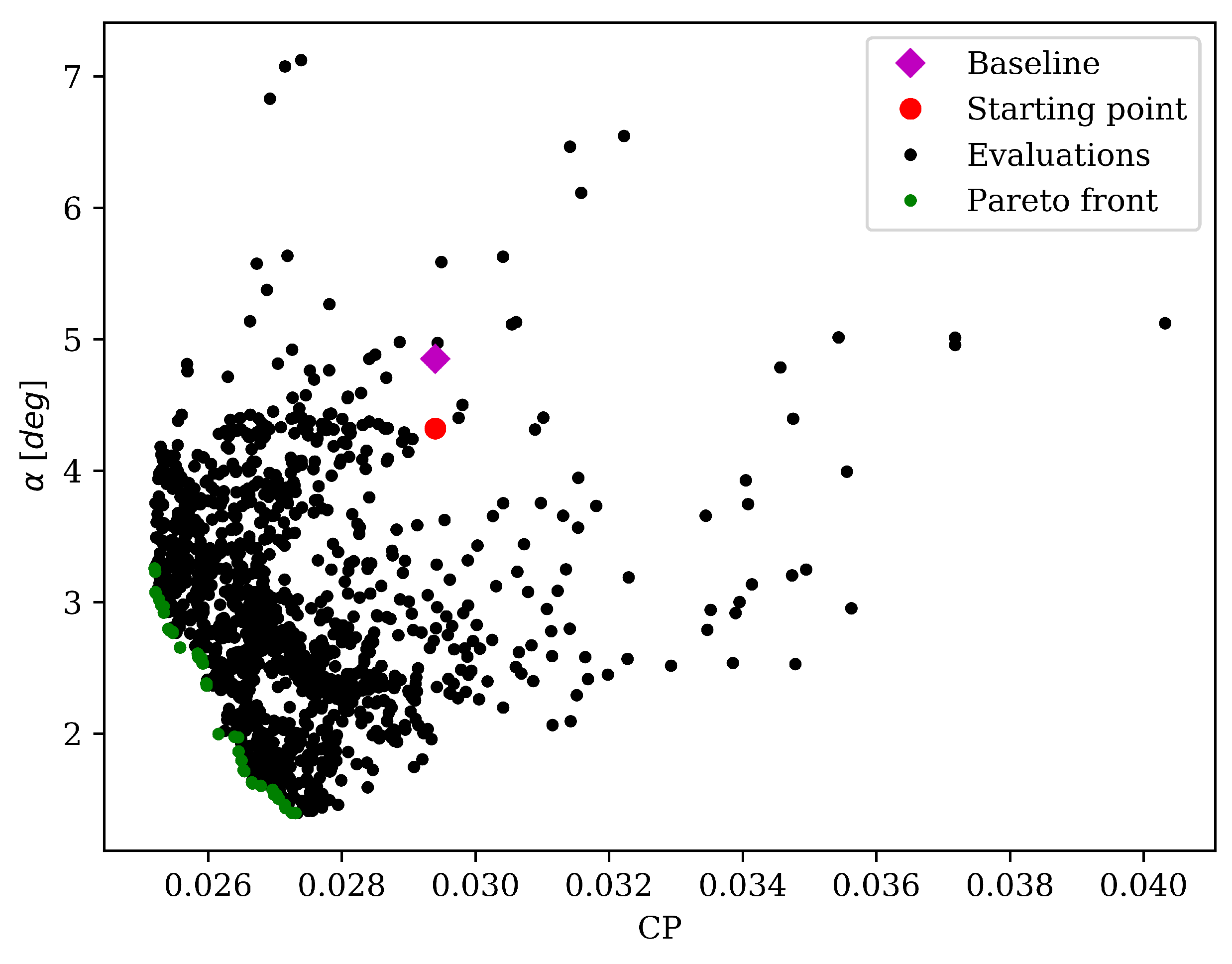
The final results of our optimization are outlined in Figure 8. The baseline objective functions are indicated with a violet diamond. As already said, this is not the optimization starting point which instead is represented by a red dot. This point represents the value of the objective function of the geometry obtained employing our new parameterization. We performed a total of 1300 evaluations which produced the Pareto front highlighted by the green dots. This result however shows some discontinuity in the Pareto front which means that not all the design space has been explored and more evaluations are needed.

Despite this, our optimization already shows remarkable results as enlighten in

Table 7. Objective functions comparison between the Baseline geometry, the extreme point and three trade-off solutions in the Pareto front.

Individual	$\mathit{CP}$	Improvement	$\mathit{\alpha }$$\left[\mathit{deg}\right]$	Improvement
Baseline (a)	$0.0294$	−	$4.8511$	−
$op{t}_{CP}$	$0.0252$	$14.3\%$	$3.2560$	$32.9\%$
$op{t}_1$	$0.0261$	$11.2\%$	$2.5216$	$48.0\%$
$op{t}_2$	$0.0262$	$10.9\%$	$1.9972$	$58.8\%$
$op{t}_3$	$0.0264$	$10.2\%$	$1.9713$	$59.4\%$
$op{t}_{\alpha }$	$0.0275$	$6.5\%$	$1.4109$	$70.9\%$

in which there are collected the objective functions value for the two extreme point and some trade-off solutions on the Pareto front. The solution with minimal total pressure losses is named $op{t}_{CP}$ and shows a reduction of about $14.3\%$ compared to the baseline geometry. The solution with minimal swirl is named $op{t}_{\alpha }$ and shows a reduction of about $70.9\%$ compared to the baseline geometry. The trade-off solutions are named $op{t}_1$, $op{t}_2$ and $op{t}_3$ and they are the point on the border of the main discontinuity in the Pareto front. $op{t}_1$ and $op{t}_2$ have similar $CP$ but different swirl angle; $op{t}_2$ and $op{t}_3$ instead has similar swirl angle and different $CP$.

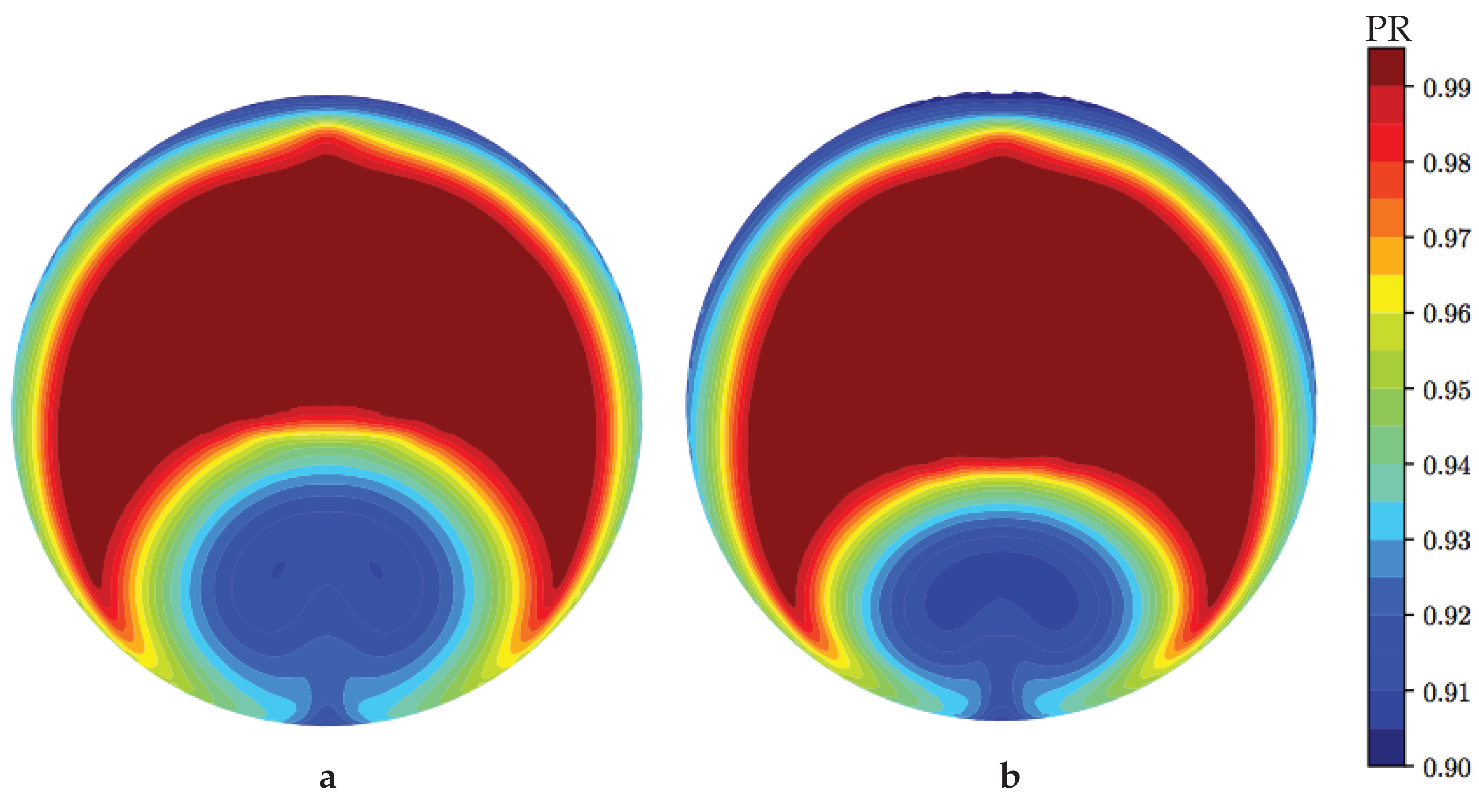
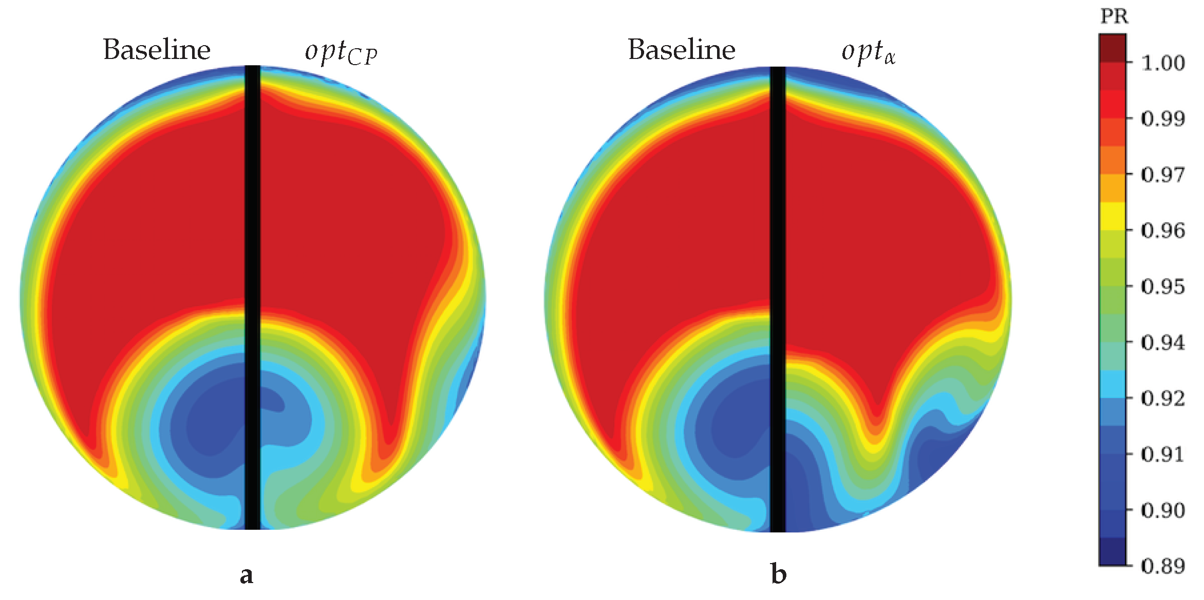
Analyzing the AIP distribution of total pressure we can see how in $op{t}_{CP}$ (Figure 9a) the low total pressure area near the lower duct portion has almost the same dimensions as the baseline, while the mean total pressure value has increased. However, a second and smaller low total pressure area appeared: its dimension is still small and its extension is confined near the external surface. Furthermore, we can see a general reduction in pressure losses near the external duct surface. If we consider now $op{t}_{\alpha }$ (Figure 9b) we can see how this second area increase in dimension to the point of equaling the main area. The latter has considerably diminished its dimensions compared to the baseline; however, the presence of this second low total pressure area frustrates any improvements.

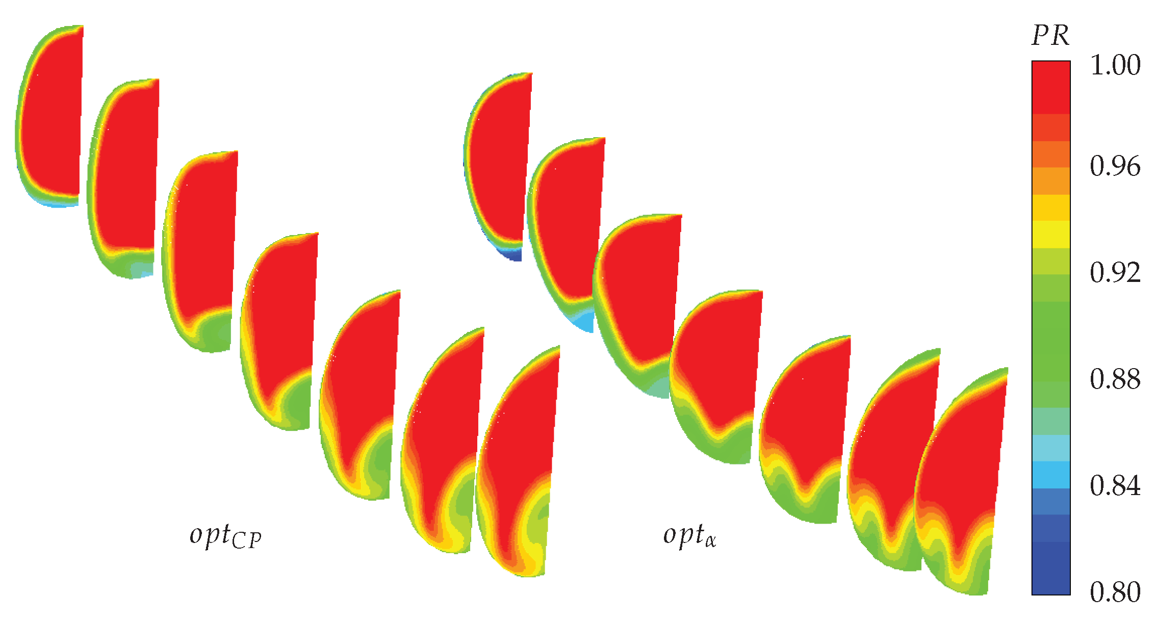
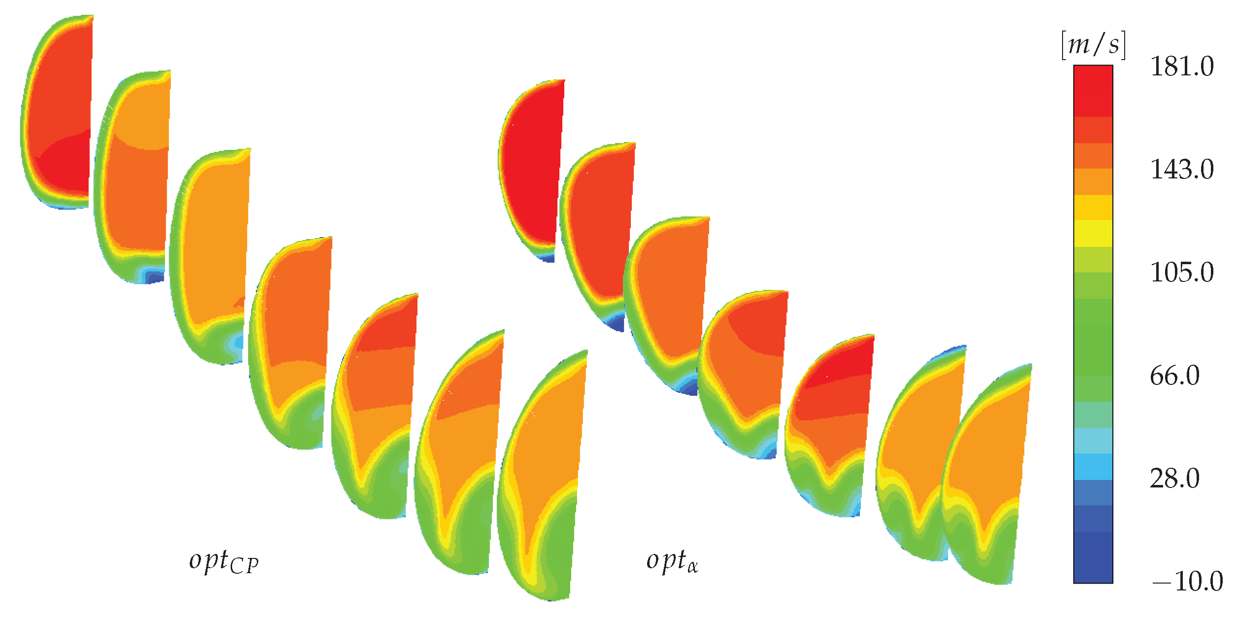
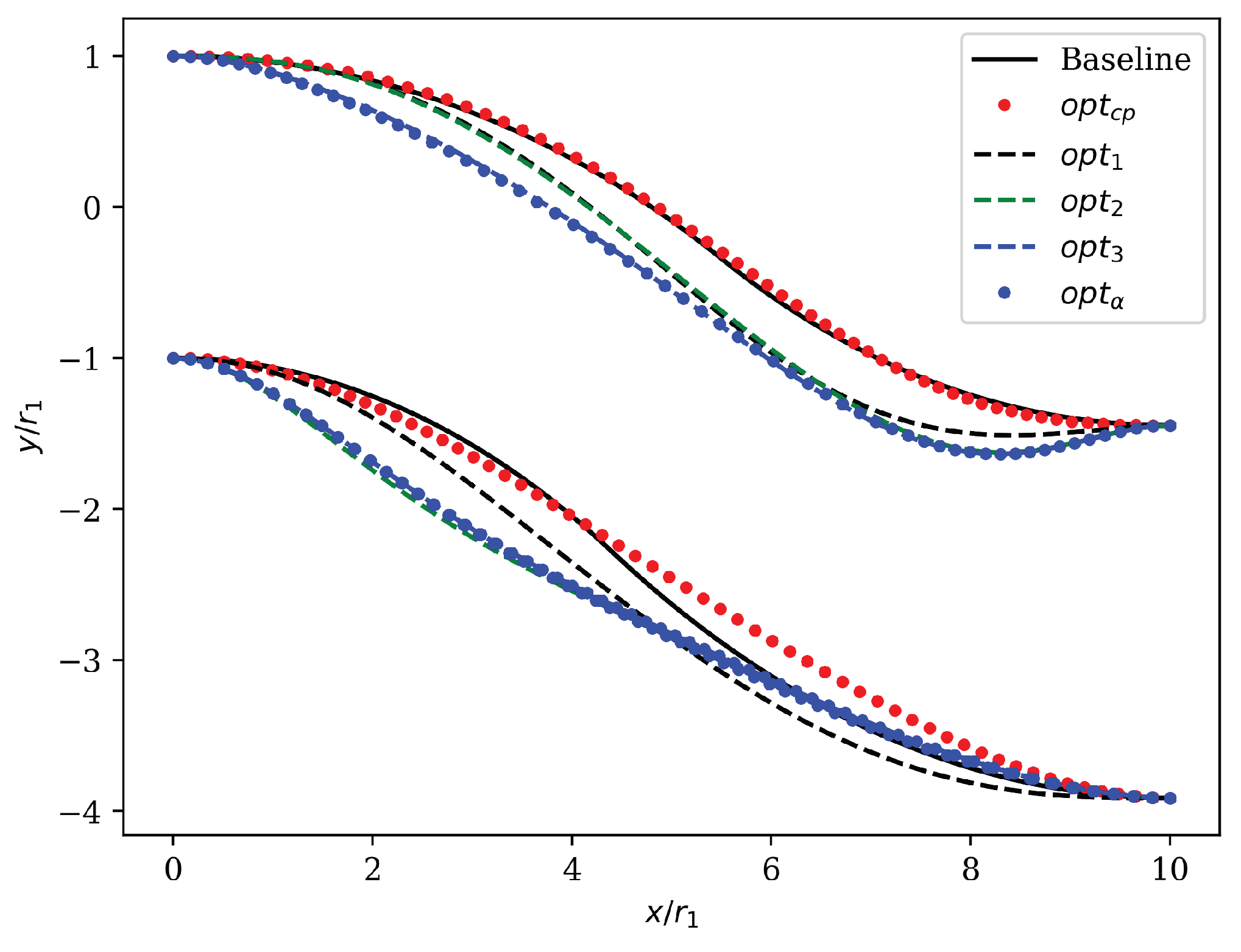
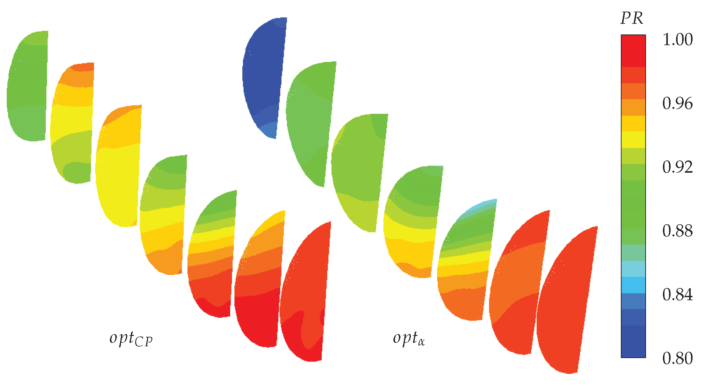
To understand this behavior we have to compare the geometry of the optimized ducts. In Figure 10 there are a series of cross-section perpendicular to x-direction from $op{t}_{CP}$ and $op{t}_{\alpha }$ showing total pressure contours. 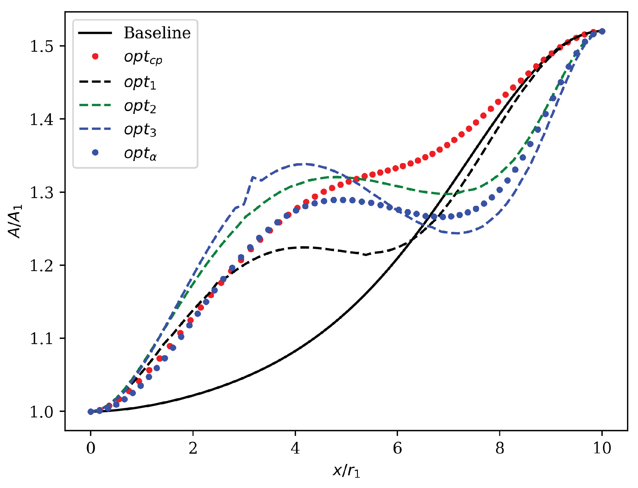The appearance of the second low total pressure region we discuss earlier occurs in the second half part of the duct and its presence is relative to the particular shape that the duct assumes in the first half part: here $op{t}_{CP}$ approaches a rectangular shape while $op{t}_{\alpha }$ approaches a triangular shape. From Figure 11 we can see that in the first half part of the duct both $op{t}_{CP}$ and $op{t}_{\alpha }$ has the same cross-section area; however, its distribution is completely different. In $op{t}_{CP}$ the area distribution is almost symmetrical with respect to $xz$-plane instead in $op{t}_{\alpha }$, since the triangular shape, the area distribution is mainly concentrated in the upper half part of the duct. To satisfy the constraint of circular cross-section at the outlet, each duct undergoes a deformation in their second half part. In correspondence of this enlargement occurs a second boundary-layer separation (Figure 12) which leads to the creation of the secondary lower total pressure region. This behavior is much more evident in $op{t}_{\alpha }$ since the transformation from triangular to circular shape in the lower part of the duct is much deeper and sudden.

In [22] a similar optimization was performed on a S-Duct with rectangular cross-section. The best solutions in terms of $CP$ reduction show values smaller than $0.05$. Even if our best $CP$ is several times greater than this result, it is interesting to note how our optimization lead to find a best solution in terms of $CP$ reduction characterized by a rectangular cross-section.

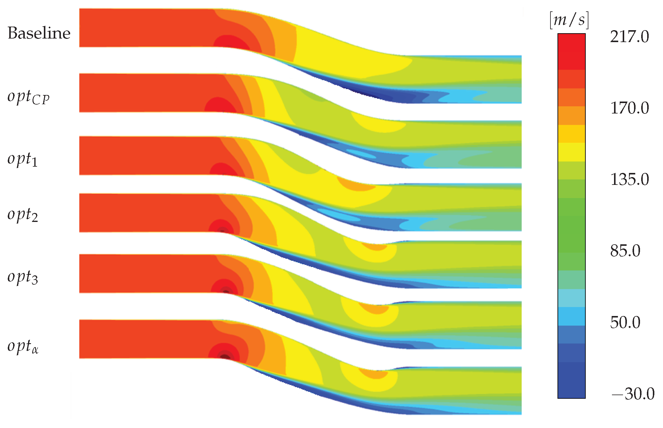
Figure 13 illustrates the axial velocity distribution on the symmetry plane: here we can observe a significant shrinking of the separation bubble for all the optimal solutions compared to the baseline. Also in this case $op{t}_{CP}$ and $op{t}_{\alpha }$ show two different behavior: while in the first case the separation region is restricted just after the first duct bent, in the second case we can see a long separation area which runs for all the S-Duct length. Despite this, it remains very narrow and adjacent to the wall. Same behavior is shown by $op{t}_2$ and $op{t}_3$, while $op{t}_1$ is much similar to $op{t}_{CP}$.

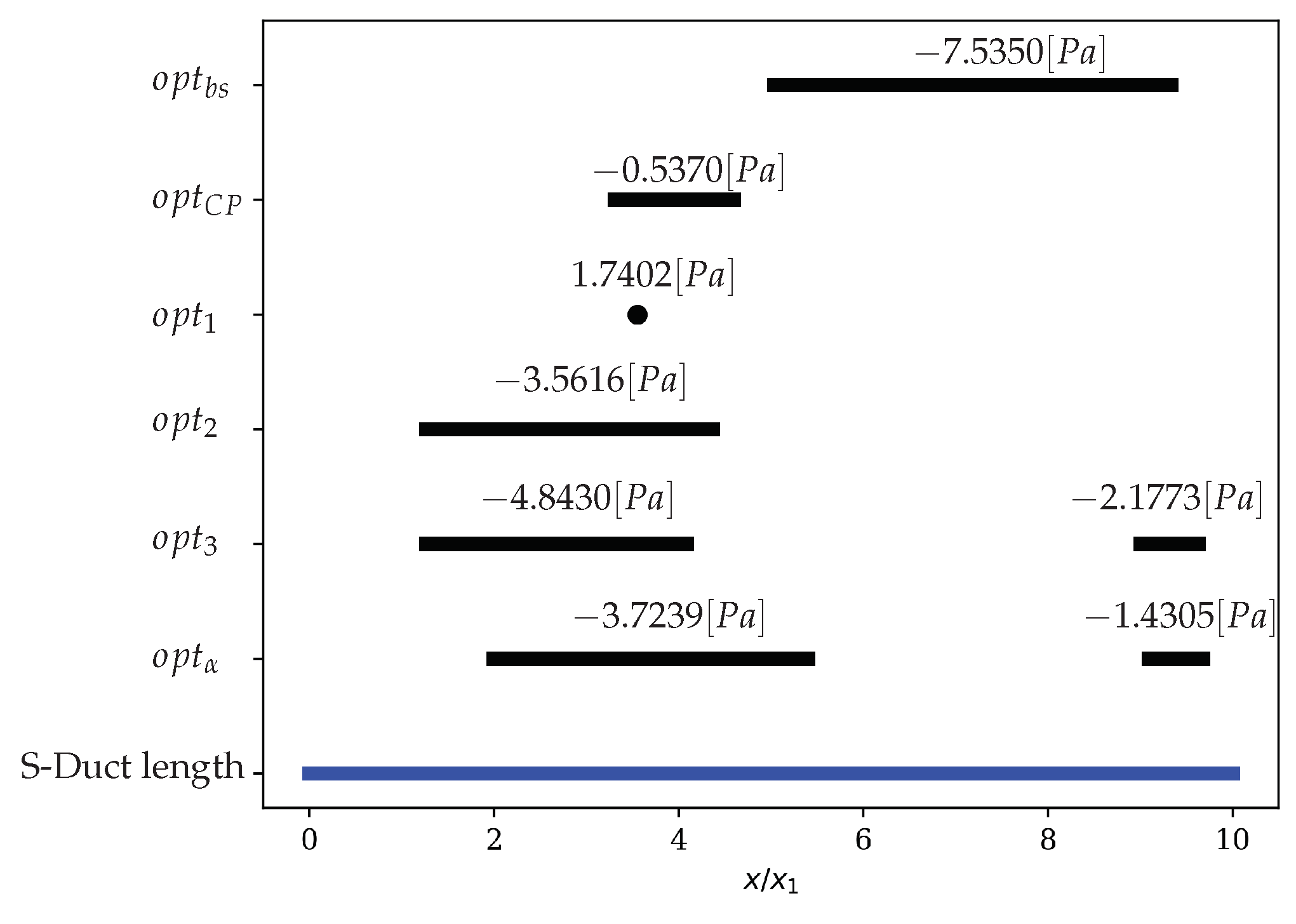
The size of the separation bubble is quantified from the distribution of the x-component of the wall shear stress on the duct wall. The length of the recirculation region is calculated as the axial length for which we detected a negative shear stress, as outlined in Figure 14. The baseline geometry shows a wide recirculation area located in the second half part of the duct. In $op{t}_{CP}$ and $op{t}_1$, instead, we can observe a reduction on the axial velocity in the lower part of the duct: $op{t}_{CP}$ shows only a small and very weak recirculation region in the first half part of the duct while $op{t}_1$ shows no recirculation at all. High flow distortions are responsible for the low total pressure area in a S-Duct. However, even if $op{t}_1$ does not show any recirculation area it is not the best solution in terms of pressure losses reduction. This is due to its cross-section shape that, like $op{t}_{\alpha }$ has, is triangular which means the presence of a second low total pressure region.

For $op{t}_2$, $op{t}_3$ and $op{t}_{\alpha }$, instead, the recirculation area is clearly evident and it occurs in the initial/central part of the duct upstream of where it occurs in the baseline. Furthermore $op{t}_3$ and $op{t}_{\alpha }$ show a secondary and weaker recirculation region towards the end of the S-Duct. Despite this, the separation region remains always very narrow and close to the duct lower wall. This behavior comes from two different geometric factors. The first is the ducts profile on the symmetry plane: the lower curve starts with a strong and fast downward bent followed by a constant slope section that ends at the outlet fitting (Figure 15). This are the reason of the early separation in comparison with the baseline. The second is the cross-section area distribution: unlike the baseline and $op{t}_{CP}$, all the other ducts present a first fast increase in the cross-section area followed by a local minimum and a second fast increase (Figure 11) characterized by a similar slope as the first part. This means that at about three quarter of these ducts there is a gauge as highlighted also by the upper line in the symmetry plane section (Figure 15). This gauge forces the flow to increase its velocity and, in particular, to decrease its static pressure through it.

To better understand this last statement we have to consider Figure 16 in which are represented the static pressure profile in different cross-section of $op{t}_{CP}$ and $op{t}_{\alpha }$. As already experimentally observed in Wellborn et al. [3,8], $op{t}_{CP}$ shows an inversion in the pressure gradient direction about halfway along the length of the duct. This explain why in this geometry (together with the baseline and $op{t}_1$) the separation region is pushed towards the upper wall continuing to increase its size. In $op{t}_{\alpha }$ instead, static pressure is almost constant in the first half part of the duct and a weaker pressure gradient with respect to $op{t}_{CP}$ appears only in the second half part. Same behavior is shown by $op{t}_2$ and $op{t}_3$. This explains both the long narrow separation region and the second separation region in $op{t}_3$ and $op{t}_{\alpha }$.

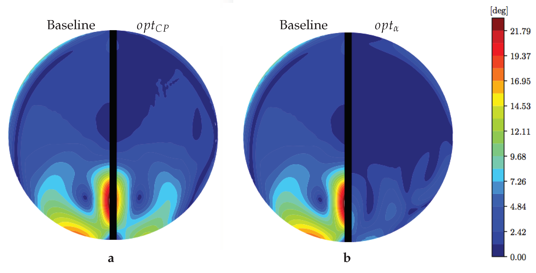
The swirl reduction is the main achievement of this numerical simulation. In fact, in $op{t}_{\alpha }$ we obtained an impressive reduction of mean swirl angle of about $70\%$ at the AIP. Here the swirl angle has a maximum value of $7.9\left[deg\right]$, almost one third with respect to the baseline ($24.3\left[deg\right]$). If we consider the contour plot at the AIP (Figure 17) we can see how $\alpha$ differs from zero only in the lower part of the duct. Furthermore $op{t}_{CP}$, even if it represents the worst solution in terms of swirl angle reduction, shows a substantial improvement of about $30\%$. 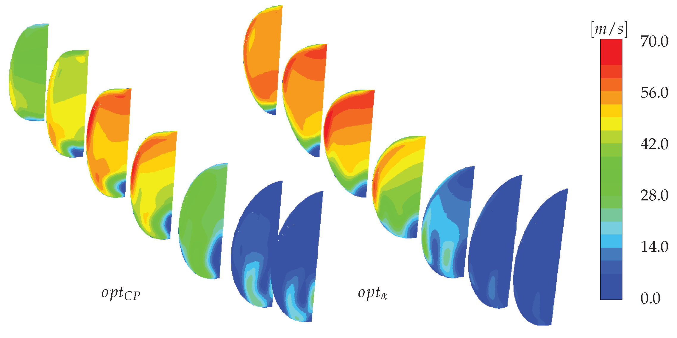Remembering the definition of swirl angle (Equation (16)), to explain this achievement we have to analyze the axial and tangential velocity distribution: all depends on the ratio of these two quantities at the AIP. In Figure 13 it is represented the axial velocity profile in different cross-section of $op{t}_{PC}$ and $op{t}_{\alpha }$. At the AIP we can observe a similar velocity distribution with the exception of presence of the second low total pressure area in the first half part of $op{t}_{\alpha }$. For that reason swirl angle is strongly linked to tangential velocity distribution.

In Figure 18 it is represented the absolute value of tangential velocity profile in different cross-section of $op{t}_{PC}$ and $op{t}_{\alpha }$. At the AIP the tangential velocity is close to zero in the upper part of both ducts. The lower part instead, is characterized by higher values due to the separation region. Here we can in fact distinguish two regions of high tangential velocity just in correspondence to the two separation regions, one on the symmetry plane and one near the external wall. The extreme low tangential velocity value in $op{t}_{\alpha }$ is, also in this case, linked to the particular triangular shape of this duct. As already said, the strong area increases in the ending and lower part of the duct due to the transition from triangular to circular cross-section implement the diffusing duct characteristic leading to an increase in static pressure and a strong reduction in tangential velocity.

4.3. Multidimensional Data Analysis of the Optimization Process

In addition to the flow analyses we performed an analysis of the whole design space of the optimization problem. This requires the simultaneous visualization of the design parameters and objective functions, which results in 38 dimensions. We use Parallel Coordinates [23] for the visualization of the multidimensional space, and the interactive approach as initially proposed in [24] and expanded in [25] for computational engineering design data.

In Figure 19 is presented the visualization of the whole history of the optimization study and a region close to the Pareto front is selected. The design parameter ×23 exhibit a particular characteristic; high values reflect the compromise region, a specific value reflects the region for the lowest swirl, and lower value reflect the region for the lowest pressure losses. Figure 20 shows the three different selections for ×23 values.

If we interactively exploit in more detail the multidimensional dataset we can identify from Figure 21 that two of the three selected optimum regions exhibit very few differences, which can be analyzed in three group of parameters, ×12 and ×13, ×23 and ×24, and ×10 (highlighted in red circles). These are when we select the compromise region and the one that exhibit the lowest swirl, flow distortion. In contrast, the region that exhibits the lowest pressure losses is expressed with considerable different combination of the design parameters, when compared to the other two regions of the Pareto front. In Figure 22 the differences between these sets of solutions are exposed and highlighted with red circles.

Hence, we can argue that two families of solutions were identified that cover the whole spectrum of optimality when we consider the flow distortion and the pressure losses.

5. Conclusions

This paper presents the computational method implemented to reduce pressure losses and flow distortion in a S-Duct. The design problem was modeled as a shape optimization study which means that the behavior of different S-Duct shapes is evaluated and compared to others considering important flow characteristics. In this case two main objective functions, that have to be minimized, were chosen: the pressure losses and the swirl. Starting from a typical S-Duct, to manage the geometry the FFD technique was employed adopting a new simple and flexible parameterization which allowed reproduction of the entire 3D duct shape with 36 decision variables. The objective functions of every deformed duct were evaluated from the result of a pressure-based steady-state RANS simulation, while the exploration of the design space was achieved using the heuristic optimization algorithm Tabu Search.

Results of this optimization are remarkable showing a reduction of about $14\%$ with respect to the pressure losses and $71\%$ with respect to the swirl angle. Compared to previous works, an extremely high improvement was achieved in terms of swirl angle, while in terms of pressure losses improvements are slightly lower. This fact is mainly due to the different parameterization approaches. The number of design variables employed in this paper are the same as in previous work, however their initial position with respect to the duct is completely different. In previous works a 3D FFD was employed embedding the duct geometry in a 3D parallelepipedic lattice. This kind of parameterization allows exact reproduction of the original geometry, however several control points are far from the duct therefore their contribution to the duct deformation is very weak. In this paper instead the entire geometry was described using only the external duct surface, which allowed description of a 3D geometry with a 2D formulation. In this way all the control points are almost on the duct external surface leading to a deeper and more flexible deformation.

Considering the optimized geometry, it is possible to distinguish two main different shapes. For geometries that show best behavior in terms of pressure losses reduction, the duct cross-section shape resembles that of a rectangle. Previous works employing a duct with a rectangular cross-section led to extremely low values of pressure losses, therefore it is interesting to note how the optimization described in this paper led to the best solution in terms of CP reduction characterized by a rectangular cross-section. Instead, the extremely high reduction in terms of swirl, which was never verified in previous works, is closely linked to a triangular duct cross-section shape. Similar geometrical characteristics describe the compromise optimum region as well. In this particular geometry the strong area increase which occurs in the ending and lower part of the duct, due to the transition from triangular to circular cross-section, exhibits the diffusing duct characteristic which leads to an overall flow slowdown.

In this paper a total of 1300 evaluations have been performed, however not all the design space has been explored since the resulting Pareto front is characterized by some discontinuity. More evaluations are needed to investigate more thoroughly the design space and obtain a more homogeneous Pareto front. Since two main cross-section shapes have emerged from this work it could be interesting in future works to study this behavior in more depth increasing the parameterization precision, i.e., the numbers of design variables. This can be achieved by introducing new cross-sections or by increasing the number of free control points in every cross-section. Finally, further higher fidelity CFD simulations could be performed in order to understand the physical behavior of such S-Duct design configurations.

The computational design methodology is well defined and flexible enough to consider additional or different models of objective function criteria. Hence, uncertainty quantification with respect to the incoming operating conditions, but also with respect to the conditions of the exit flow, could be considered in future studies.

References

1. Liebeck, R.H. Design of the Blended Wing Body Subsonic transport. J. Aircr. 2004, 41, 10–25. [Google Scholar] [CrossRef]
2. Vakili, A.; Wu, J.-Z.; Liver, P.; Bhat, M.K. Measurements of compressible secondary flow in a circular S-duct. In Proceedings of the AlAA 16th Fluid and Plasma Dynamics Conference, Danvers, MA, USA, 12–14 July 1983. [Google Scholar]
3. Wellborn, S.R.; Reichert, B.A.; Okiishi, T.H. An experimental investigation of the flow in a diffusing S-Duct. In Proceedings of the 28th Joint Propulsion Conference and Exhibit, Nashville, TN, USA, 6–8 July 1992. [Google Scholar]
4. Delot, A.L.; Garnier, E.; Pagan, D. Flow control in a high-offset subsonic air intake. In Proceedings of the 47th AIAA/ASME/SAE/ASEE Joint Propulsion Conference & Exhibit, San Diego, CA, USA, 31 July–3 August 2011. [Google Scholar]
5. Gissen, A.N.; Vukasinovic, B.; McMillan, M.L.; Glezer, A. Distortion management in a BLI inlet diffuser using synthetic-jet hybrid flow control. In Proceedings of the 49th AIAA Aerospace Sciences Meeting including the New Horizons Forum and Aerospace Exposition, Orlando, FL, USA, 4–7 January 2011. [Google Scholar]
6. Chiereghin, N.; Guglielmi, L.; Savill, M.; Kipouros, T.; Manca, E.; Rigobello, A.; Barison, M.; Benini, E. Shape Optimization of a Curved Duct with Free Form Deformations. In Proceedings of the 23rd AIAA Computational Fluid Dynamics Conference, Denver, CO, USA, 5–9 June 2017. [Google Scholar]
7. Tridello, R. Comparison of Genetic and Tabu Search Algorithms in Aerodynamic Design of S-Duct. Master’s Thesis, Cranfield University, Cranfield, UK, 2017. [Google Scholar]
8. Wellborn, S.R.; Okiishi, T.H.; Reichert, B.A. A Study of the Compressible Flow Through a Diffusing S-Duct; NASA Technical Memorandum 106411; NASA Lewis Research Center: Cleveland, OH, USA, 1993.
9. Zachos, P.; MacManus, D.G.; Chiereghin, N. Flow distortion measurements in convoluted aero engine intakes. In Proceedings of the 33rd AIAA Applied Aerodynamics Conference, Dallas, TX, USA, 22–26 June 2015. [Google Scholar]
10. Chiereghin, N.; MacManus, D.G.; Savill, M.; Dupuis, R. Dynamic distortion simulations for curved aeronautical intakes. In Proceedings of the Advanced Aero-concepts, Design and Operations, Royal Aeronautical Society Applied Aerodynamics Conference, Bristol, UK, 22–24 July 2014. [Google Scholar]
11. MacManus, D.G.; Chiereghin, N.; Gil Prieto, D.; Zachos, P. Complex aero-engine intake ducts and dynamic distortion. In Proceedings of the AIAA Aviation and Aeronautics Forum and Exposition, Dallas, TX, USA, 16–20 June 2014. [Google Scholar]
12. Deb, K. Multi-Objective Optimization Using Evolutionary Algorithms; Wiley: Hoboken, NJ, USA, 2001. [Google Scholar]
13. Toffolo, A.; Benini, E. Genetic diversity as an objective in multi-objective evolutionary algorithms. Evolut. Comput. 2003, 11, 151–167. [Google Scholar] [CrossRef] [PubMed]
14. Da Ronco, C.C.; Benini, E. A simplex crossover based evolutionary algorithm including the genetic diversity as objective. Appl. Soft Comput. 2001, 13, 2104–2123. [Google Scholar] [CrossRef]
15. Jaeggi, D.M.; Parks, G.T.; Kipouros, T.; Clarkson, P.J. The development of a Multi-Objective Tabu Search algorithm for continuous optimisation problem. Eur. J. Oper. Res. 2008, 185, 1192–1212. [Google Scholar] [CrossRef]
16. Delot, A.L.; Scharnhorst, R.K. A comparison of several CFD codes with experimental data in a diffusing S-Duct. In Proceedings of the 49th AIAA Joint Propulsion Conference, San Jose, CA, USA, 15–17 July 2013. [Google Scholar]
17. Sederberg, T.W. Free-form deformation of solid geometric models. ACM Siggraph Comput. Graph. 1986, 20, 151–160. [Google Scholar] [CrossRef] [Green Version]
18. Peachey, T.C.; Kipouros, T. Nimrod/O User’s Guide; Monash University: Melbourne, Australia, 2013. [Google Scholar]
19. Gil-Prieto, D.; MacManus, D.G.; Zachos, P.K.; Tanguy, G.; Menzies, K.R. Convoluted Intake Distortion Measurements Using Stereo Particle Image Velocimetry. AIAA J. 2017, 55, 3560. [Google Scholar] [CrossRef]
20. Gil-Prieto, D.; MacManus, D.G.; Zachos, P.K.; Tanguy, G.; Wilson, F.; Chiereghin, N. Delayed Detached-Eddy Simulation and Particle Image Velocimetry Investigation of S-Duct Flow Distortion. AIAA J. 2017, 55, 1893–1908. [Google Scholar] [CrossRef]
21. Fiola, C.; Agarwal, K.R. Simulation of Secondary and Separated Flow in Diffusing S Ducts. AIAA J. Propuls. Power 2015, 31, 180–191. [Google Scholar] [CrossRef]
22. Furlan, F.; Chiereghin, N.; Kipouros, T.; Benini, E.; Savill, M. Computational design of S-Duct intakes for distributed propulsion. Aircr. Eng. Aerosp. Technol. Int. J. 2014, 86, 473–477. [Google Scholar] [CrossRef]
23. Inselberg, A. Parallel Coordinates: Visual Multidimensional Geometry and Its Applications; Springer: Berlin, Germany, 2009. [Google Scholar]
24. Kipouros, T.; Mleczko, M.; Savill, M. Use of Parallel Coordinates for Post-Analyses of Multi-Objective Aerodynamic Optimisation in Turbomachinery. In Proceedings of the AIAA Multidisciplinary Design Optimization Specialist Conference, Schaumburg, IL, USA, 7–10 April 2008. [Google Scholar]
25. Kipouros, T.; Inselberg, A.; Parks, G.T.; Savill, M. Parallel Coordinates in Computational Engineering Design. In Proceedings of the AIAA Multidisciplinary Design Optimization Specialist Conference, Boston, MA, USA, 8–11 April 2013. [Google Scholar]
Figure 1. Optimization loop.
Designs 02 00036 g001
Figure 2. S-Duct scheme.
Designs 02 00036 g002
Figure 3. Parallelepipedic lattice defined on a plane surface in the symmetry plane (plane x y ) of the S-Duct. Dotted lines represent the duct projection on this plane: curves define the main lattice dimensions.
Designs 02 00036 g003
Figure 4. Generic cross-section. The black semicircular line represents the baseline geometry. The blue line represents the deformed geometry when the control points P 1 P 6 are equally spaced on the baseline geometry section.
Designs 02 00036 g004
Figure 5. (a) PR and (b) α as a function of the number of mesh elements. The red solid line in (a) represent the experimental result form [16].
Designs 02 00036 g005
Figure 6. Cross-section mesh topology.
Designs 02 00036 g006
Figure 7. Baseline pressure recovery distribution comparison: (a) CFD simulation with same geometry as in [16]; (b) CFD simulation with geometry obtained from our new parameterization.
Designs 02 00036 g007
Figure 8. The Pareto front and the history of the optimization study.
Designs 02 00036 g008
Figure 9. Total pressure distribution at AIP. (a) Comparison between Baseline and o p t C P . (b) Comparison between Baseline and o p t α .
Designs 02 00036 g009
Figure 10. Total pressure distribution in different cross-section: comparison between o p t C P (left) and o p t α (right). Every cross-section is perpendicular to x-direction and situated at x = 2.5 r 1 , x = 4 r 1 , x = 5.5 r 1 , x = 7 r 1 , x = 8.5 r 1 , x = 10 r 1 (S-Duct outlet) and x = 11 r 1 (AIP) from S-Duct inlet.
Designs 02 00036 g010
Figure 11. S-Duct cross-sections area in optimized solutions compared with Baseline. y-axis represent the ration between the area of the generic cross-section perpendicular to x-direction and inlet area.
Designs 02 00036 g011
Figure 12. Axial velocity distribution in different cross-section: comparison between o p t C P (left) and o p t α (right). Every cross-section is perpendicular to x-direction and situated at x = 2.5 r 1 , x = 4 r 1 , x = 5.5 r 1 , x = 7 r 1 , x = 8.5 r 1 , x = 10 r 1 (S-Duct outlet) and x = 11 r 1 (AIP) from S-Duct inlet.
Designs 02 00036 g012
Figure 13. Axial velocity distribution on symmetry plane in optimized solutions compared with Baseline.
Designs 02 00036 g013
Figure 14. Recirculation region in optimized solutions compared with Baseline. Blue line represent the total S-Duct axial length. Black lines represent the axial length of recirculation region. Numbers over each lines states the minimum values of x-wall shear stress. Black dot in correspondence of o p t 1 indicates the position of the minimum (positive) value of x-wall shear stress for that geometry.
Designs 02 00036 g014
Figure 15. S-Duct geometry on symmetry plane in optimized solutions compared with Baseline.
Designs 02 00036 g015
Figure 16. Static pressure distribution in different cross-section: comparison between o p t C P (left) and o p t α (right). Every cross-section is perpendicular to x-direction and situated at x = 2.5 r 1 , x = 4 r 1 , x = 5.5 r 1 , x = 7 r 1 , x = 8.5 r 1 , x = 10 r 1 (S-Duct outlet) and x = 11 r 1 (AIP) from S-Duct inlet.
Designs 02 00036 g016
Figure 17. Swirl angle distribution at AIP. (a) Comparison between Baseline and o p t C P . (b) Comparison between Baseline and o p t α .
Designs 02 00036 g017
Figure 18. Absolute value of tangential velocity distribution in different cross-section: comparison between o p t C P (left) and o p t α (right). Every cross-section is perpendicular to x-direction and situated at x = 2.5 r 1 , x = 4 r 1 , x = 5.5 r 1 , x = 7 r 1 , x = 8.5 r 1 , x = 10 r 1 (S-Duct outlet) and x = 11 r 1 (AIP) from S-Duct inlet.
Designs 02 00036 g018
Figure 19. The complete dataset is represented in Parallel Coordinates and the two objective functions in the Scatter plot. A selection of the Pareto front is highlighted in blue.
Designs 02 00036 g019
Figure 20. Three interval selections expressed for design parameter ×23 and the reflection to the regions of optimality close to the Pareto front.
Designs 02 00036 g020
Figure 21. Comparison between the groups of solutions in the compromise region and extreme optimality for the swirl objective function (highlighted in blue).
Designs 02 00036 g021
Figure 22. Comparison between the groups of solutions in the compromise region (highlighted in blue) and extreme optimality for the pressure loss objective function.
Designs 02 00036 g022