1. Introduction
Remote sensing plays a vital role in smart agriculture. Using sensors, it collects information about soil conditions, weather conditions, humidity, and crop health, and contributes to food security and sustainable development [
1,
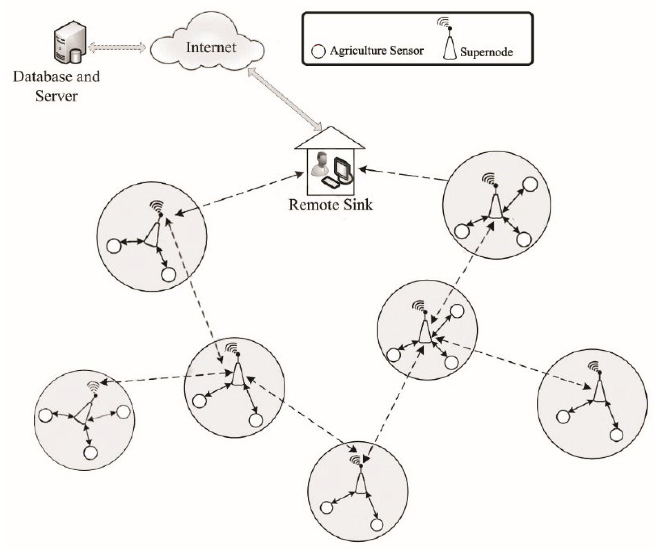
2]. Smart agriculture uses a series of equipment, such as agricultural sensors, actuators, and drones, which are connected through wireless communication. WSN is the most significant component in smart agriculture, and is used in soil analysis, weather monitoring, determining yield productivity, the early detection of disease, and crop monitoring.
Figure 1 shows an example of this architecture. In these systems, agricultural sensors should cover the entire environment during network activity to fully monitor crops. Thus, network connectivity is the primary challenge in this area. Each node failure can cause the disconnection of a series of other sensors from the network, so fault tolerance in WSN-based smart agriculture is a solution for high network connectivity. Additionally, other significant challenges, such as data traffic unbalancing, energy consumption, node damping near sinks, and environment factors lead to failure in these networks [
3]. All the above challenges regarding high network connectivity should be solved so they do not negatively affect the efficiency of the smart agriculture system.
The preceding challenges can be overcome by developing a wireless sensor and actuator network (WSAN), where supernodes serve as alternative gateways that are the core of the WSAN [
4]. In addition to broader transmission ranges and more excellent batteries, supernodes perform the decision making process and make specific reactions based on their decisions. In many cases, data delivery from nodes to these supernodes is sufficient to ensure the network functions correctly [
5,
6]. According to [
7], optimizing the placement of supernodes can extend the network lifetime by a factor of five. These networks can also be used for different purposes, e.g., recognizing combustion in agriculture [
8], underground precision agriculture [
9], and olive grove monitoring [
10].
Studies indicate that traffic load and energy consumption distribution pose challenges for heterogeneous wireless sensor networks. Inefficient distributions result in a situation where, following the failure of the initial network node, 90% of the energy in live nodes remains unused [
11]. Many studies attempted to balance the energy consumption of nodes so that they would discharge at a specific interval through different methods, e.g., by using a dynamic transmission range and adjusting the transmission range [
12]. Earlier works reported that balancing energy consumption can improve the network’s lifetime by 30% since it helps balance the data traffic in the nodes adjacent to the sink [
13]. Consequently, the proposed path construction method considers the residual energy of path-forming nodes as a crucial parameter, with nodes of a lower energy contributing to fewer paths.
Hotspots, or bottlenecks, are nodes that exist at a one-step distance from supernodes. Their energy discharges much more rapidly than that of other nodes since they serve as relay nodes for other nodes in addition to sending sensed data. Thus, hotspot failure is a significant challenge for sensor networks since it disconnects many nodes from supernodes [
14,
15,
16]. Numerous studies have analyzed supernode mobility [
14,
15,
17,
18] and clustering [
19,
20,
21,
22,
23,
24,
25] to overcome this challenge. The energy consumption of relay nodes can be balanced through supernode mobility and the periodic change of relay nodes. However, a mobile supernode imposes a new challenge on the network since a new movement and settlement change the network topology. Control messages are required to arrange a new topology to provide network coverage and connectivity. Therefore, handling the premature damping of relay nodes leads to the control message overhead in the network. Furthermore, finding optimal settlement points for a supernode is an NP-hard problem [
26]. In [
27], a suboptimal heuristic algorithm was assessed to find settlement points. The preceding techniques have the drawback of focusing primarily on the relay nodes while ignoring the other nodes’ energy consumption.
Agriculture sensors may fail for various reasons, such as energy discharge, hardware faults, and severe weather. This failure can disconnect a series of nodes from the network. It is essential to design fault-tolerant methods for network re-connectivity. In the disjoint path vector (DPV) method [
6], each node is connected to a set of supernodes through
k-disjoint paths to enable a node to select other paths to transmit the sensed data in case of node failure. DPV is aimed at reducing the total transmission range and maximum transmission range in order to lengthen the network’s lifetime. It can maintain supernode connectivity at a node failure rate of up to 5% [
5,
28]. In DPV, a node failure reduces
k-vertex connectivity, whereas a supernode failure disconnects a large number of nodes. In [
5], the adaptive disjoint path vector (ADPV) utilized
r-restoration paths to maintain
k-vertex connectivity. Despite improved supernode connectivity, it had two significant disadvantages: (1) the supernode layer was not fault-tolerant, and supernode failure disconnected a large number of nodes; (2) hotspots were required to be much more than
k in number to avoid bottlenecks and premature death. In other words, ADPV was heavily dependent on the network structure and node locations in an operating environment.
This paper introduces a scheme for connectivity restoration, a two-layered fault-tolerant system, and a dynamic clustering method designed for heterogeneous wireless sensor network-based smart agriculture. The primary aim is to enhance quality of service (QoS) by improving connectivity restoration through the establishment of connections between individual nodes and m-supernodes using k-disjoint paths. Additionally, the proposal seeks to augment resilience to node and supernode failures by adjusting transmission powers and dynamically clustering sensors based on residual energy. Furthermore, it aims to prolong network lifetime by strategically positioning relay nodes as migration points for mobile supernodes.
The following is an overview of this paper’s primary contributions:
By considering residual energy levels in path-construction nodes, the design facilitates efficient data transfer from low-energy to high-energy nodes. This approach aims to optimize network lifetime and load balancing.
By preventing the transmission of control messages that do not impact neighboring path tables, the proposed method optimizes the use of control messages, leading to improved network efficiency and lower congestion.
By designing a distributed and energy-aware methodology, a robust topology is built to tolerate up to k − 1 node failures and m − 1 supernode failures, greatly increasing network connectivity.
By dynamically reassigning nodes to secondary supernodes based on the longest path lifetime, in the event of a primary supernode failure, the system ensures fault tolerance and network connectivity.
By implementing an optimal greedy algorithm to identify migration points from relay nodes, this strategy relocates supernodes strategically. This design leads to distributing traffic load, enhancing fault tolerance by preventing relay node failures, and improving network lifetime through efficient supernode movement and settlement.
This study is divided into several sections.
Section 2 reviews the study literature, and
Section 3 presents the suggested solution and algorithms. The evaluation findings are presented in
Section 4, and a conclusion is drawn in
Section 5.
2. Literature Review
Based on the predictions, the world population will reach one billion people by 2050 [
29]. This population growth requires a sustainable proportional increase in crops. Also, it is estimated that the number of people with cancer will be about 26 million by 2030 [
30], and 17 million people will die from this disease. Food security is one of the ways to prevent this disease. Remote sensing plays a vital role in modern agriculture since it can effectively provide and improve food security and sustainable crop growth by monitoring the quality and quantity of crops. Moreover, the application of remote sensing, especially in its water-related contexts, has the potential to furnish sustainable resolutions for addressing the imminent challenge of irrigation water scarcity [
31]. The infrastructure of these systems is wireless sensor networks. The challenges of WSN-based smart agriculture should be solved for better crop management. This section presents an overview of the recent studies on fault tolerance topology control, clustering methods, mobile supernodes, heterogeneity, and connectivity restoration.
Fault tolerance is an essential task in WSNs, ensuring uninterrupted data exchange. In recent years, many studies have been conducted on fault tolerance topology control [
32,
33,
34,
35] to reduce the residual energy consumption of nodes by adjusting the transmission power. In [
36], a distributed topology control method was proposed for a WSN to change its topology dynamically through network coding. In [
34], the game algorithm was employed to design a fault-tolerant topology control scheme for underwater WSNs by reducing unnecessary links and energy consumption. In [
37], clustering was combined with fault tolerance to reduce energy consumption by applying fault tolerance to inter-cluster links. Fault tolerance and clustering were integrated in [
38], using particle swarm optimization (PSO) to connect the members of a failed cluster to the new cluster head. These methods mainly focus on topology control and clustering to reduce node energy consumption. They ensure fault tolerance by lowering energy consumption.
Designing clustering algorithms is a method of reducing energy consumption in WSNs. Cluster head selection has been recently discussed in many studies. In [
39], residual energy, node density, and node distances from sinks were integrated, and a fuzzy system was employed to calculate the probability of node selection as cluster heads. In addition to these parameters, link lifetime was considered in [
40], assigning specific weights to each parameter. The residual energy had the highest weight, whereas the sink distance had the lowest weight. In [
41], a PSO-based method was adopted to find the optimal cluster head by combining residual energy and sink distance to minimize the message overhead. In [
42], nodes were clustered before using energy-based paths to connect clusters. In [
43], the adaptive selfish optimization algorithm was utilized to select cluster heads, and the
k-medoids technique was used to determine the nodes of each cluster to lengthen the network’s lifetime by preserving node energy. In [
44], each UAV was considered a cluster head by default, and hierarchical clustering was employed to transmit data to UAVs. In actuality, clustering algorithms distribute network nodes over various zones; hence, cluster heads and inter-cluster routes should include fault tolerance to prevent network disconnectivity. These techniques only considered energy usage and lacked fault tolerance.
Mobile sinks are a standard method to distribute relay jobs between nodes since such mobility can periodically change the relay nodes. In [
45], the main focus was on reducing the sink travel distance, and path planning was used to shorten the traveled distance of sinks. In [
46], the primary purpose was to lengthen the network’s lifetime. To balance traffic load distribution, the relay nodes were periodically changed by utilizing sink movement between clusters.
In [
47], mobile sinks and clustering were integrated; the sink was mounted on the cluster head with the highest traffic load in the subsequent migration. In [
48], two important parameters were measured: movement time and stop time. The sink moved to the next migration at the movement time and remain there for the stop time. In [
49], an ant colony optimization-based algorithm was proposed, where each node selected a data-gathering point via a random function. These data-gathering points determined the sink settlement points. In [
50], a bipartite graph was created to divide sensor nodes into two sets, and the mobile sink calculated the nearest neighboring node using the breadth-first traversal algorithm once it entered each set. Then, it visited the node in the next movement. These methods focused mainly on collecting sensor data, decreasing energy consumption, and neglecting fault tolerance.
Regarding connectivity restoration in WSAN, the DPV algorithm [
6] is designed to decrease the total transmission power in heterogeneous wireless sensor networks by maintaining the
k-vertex disjoint paths from each sensor to a group of supernodes. Generally, this algorithm’s input is a
k-vertex supernode-connected graph, and its output is a subgraph with fewer edges composed of the same collection of sensors. This method finds the edges that satisfy the following conditions:
ADPV [
5] extends the DPV algorithm and uses the residual energy of sensor nodes to generate a fault-tolerant topology. This method improves the network’s lifetime by balancing the energy consumption of sensor nodes and involving initialization and restoration phases. In the first phase, the necessary information is collected, and the initial topology is constructed. In ADPV, whenever a node failure disrupts the connectivity of the
k-vertex supernode, other
k-disjoint paths are extracted for each sensor node during the restoration phase. At the end of the restoration phase, the transmission power of each node is adjusted in the generated topology. The disadvantage of the studies reviewed by [
5,
6] is that they considered only node failures; however, network connectivity may also be affected by supernode failures. In these methods, sensor nodes and supernodes are static; hence, they are ineffective in prolonging the network’s lifetime. The suggested approach to increasing network lifetime involves mobilizing supernodes and considering their failures.
3. The Proposed Method
This section introduces k-disjoint paths to m-mobile supernodes (KDPMS). In the worst case, this approach can tolerate k − 1 node and m − 1 supernode failures and balance relay jobs between the nodes. KDPMS also manages connectivity by changing the transmission power of nodes and clustering the sensor nodes dynamically. It merely requires messaging with one-step neighbors to construct a topology.
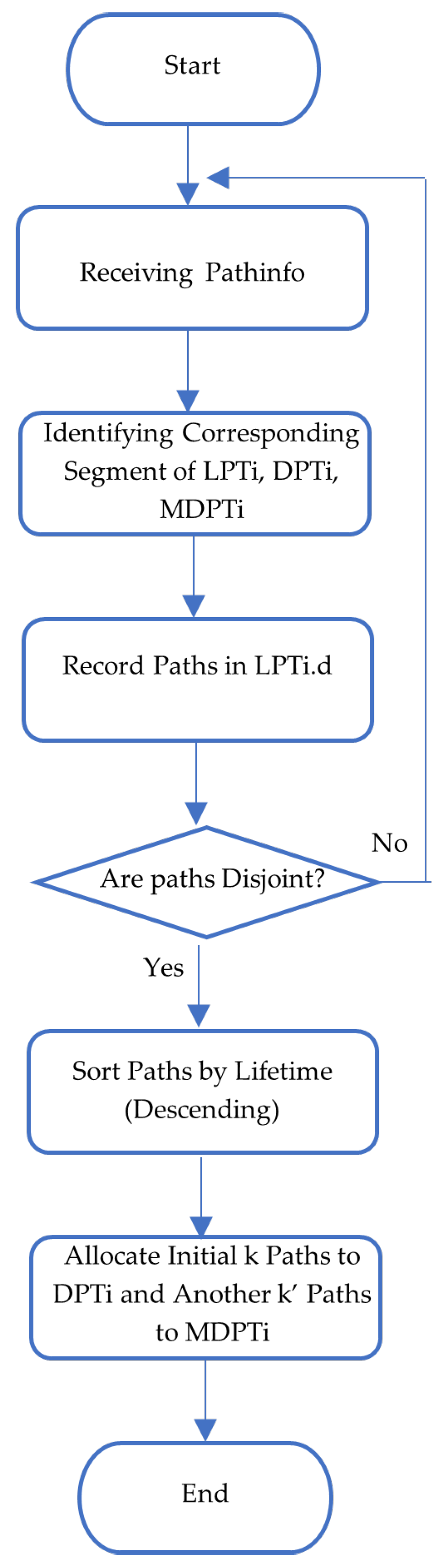
The flowchart in
Figure 2 helps to describe the proposed algorithms and theorems. In this method, three tables are required for each node, e.g., a local path table (LPT), disjoint path table (DPT), and maintenance disjoint path table (MDPT). These tables are organized into
m +
m′ ⊂
Ns segments, where
Ns represents a set of supernodes, and each segment details paths to a specific supernode with their respective lifetimes. Within each DPT segment,
k-disjoint paths are arranged by lifetime, leading to a designated supernode. DPT
i encompasses all paths in segment
i, while DPT
i…j includes segments
i to
j of the DPT. Additionally, DPT
i.d denotes the supernode ID in segment
i, and DPT
i,j signifies path
j of segment
i. The initial
m segments of the DPT establish connections to
m supernodes, while the subsequent
m′ segments are employed for the preservation of
m-supernode connectivity. Notably, there are
kλ nodes in DPT
i, where
λ denotes the longest path length. Furthermore, the total numbers of paths and nodes in the DPT are
k(
m +
m′) and
kλ(
m +
m′), respectively.
Each segment of the MDPT contains k′-disjoint paths aimed at restoring k-vertex connectivity. When a node failure removes a path from DPTi, the path of the longest lifetime in MDPTi takes its place. It is crucial for proper network operation that for all of i, DPTi.d equals MDPTi.d. In MDPTi, there are k′λ nodes, and the total numbers of paths and nodes in the MDPT are represented as k′(m + m′) and k′λ(m + m′), respectively.
Upon receiving new path information from immediate neighbors with supernode destination d, these paths are recorded in LPTi.d. Following the confirmation of their disjoint nature, the paths are organized in descending order based on their lifetimes. The initial k paths, possessing the longest lifetimes, are allocated to DPTi, while the remaining k′ paths find placement in MDPTi. Subsequently, DPT organizes its segments by lifetime, ensuring ∀i (lifetime (DPTi) > lifetime (DPTi+1)). DPT1 holds disjoint paths to the primary supernode, while DPT2…m contains disjoint paths to secondary supernodes. The alternative supernodes are utilized to reinstate m-supernode connectivity from the ensuing m′ segments. The optimal disjoint paths are identified by determining the path lifetime based on the residual energy of their nodes, as per Equation (A7).
KDPMS is structured into five distributed algorithms. During Algorithms 1 and 2, denoted as path information collection, each node undertakes the extraction of k-optimal disjoint paths and k′-optimal maintenance disjoint paths for individual segments. This process involves the acquisition of path information from adjacent one-step neighboring nodes, resulting in a topology characterized by k-disjoint paths to m-mobile supernodes. Inspired by the algorithms employed in DPV and ADPV, this study introduces a nuanced yet impactful modification aimed at minimizing the number of control messages. Within this framework, every supernode assumes the role of a cluster head, and each agricultural node is integrated as a member of the corresponding supernode cluster, as identified within DPT1.d. The algorithm is designed to optimize network lifetime, facilitate load balancing, and enhance network connectivity.
Algorithm 3 is enacted in response to a node failure, disrupting k-vertex connectivity. In such situations, k′-disjoint paths within MDPTi are utilized to restore k-vertex connectivity. It is important to note that each node failure leads to adjustments in the DPT and MDPT of nodes with paths involving the failed node. In the event of a supernode failure, Algorithm 4 is initiated, employing m′-alternative supernodes to preserve m-supernode connectivity. In this approach, supernode i is designated as a cluster head, and the node with the longest path lifetime to supernode i is assigned to cluster i. In the event of a cluster head failure within a node, the imperative is for the node to dynamically designate an alternate cluster head, guided by considerations of the path’s lifetime to the new cluster head. These algorithms play a crucial role in ensuring fault tolerance and sustaining network connectivity.
Algorithm 5 confronts the challenges of identifying optimal supernode migration points and the supernode settlement time at these points, and establishing the next migration point. During this algorithm, an initial assumption is made that the locations of supernodes are static, and migration points are determined through the implementation of an optimal greedy algorithm applied to the dominating set problem. The migration points are selected from the relay nodes, and the supernodes are mounted on these nodes during their movements. This strategic process aims to mitigate the risk of relay node failures, consequently enhancing fault tolerance and prolonging the network’s lifetime.
3.1. Problem Statement
Initiating our discourse, we present the formal elucidation of k-vertex to m-supernode connectivity.
Definition 1. Disjoint Paths [6]: Disjoint paths are paths with common ends but distinct middle nodes. Definition 2. k-Vertex to m-Supernode Connectivity [51]: Achieving k-vertex to m-supernode connectivity in a heterogenous wireless sensor network depends on ensuring that removing k − 1 nodes will not disconnect any nodes from their respective supernodes. Similarly, the removal of m − 1 supernodes will not disconnect any nodes from the overall network structure. In the initial configuration, we are given a network characterized by k-vertex to m-supernode connectivity, encompassing Ns supernodes and N sensor nodes. The transmission range of sensor nodes is subject to adjustment within the constraints of a predefined constant denoted as Rmax. By incorporating models of node and supernode failures, the count of active agriculture sensor nodes and supernodes diminishes over the network’s operational duration. Notably, we employ N(t) to represent the set of active agriculture sensor nodes and Ns(t) to denote active supernodes at a given time, t, measured in discrete intervals. The primary objective lies in determining the transmission ranges of all active sensor nodes at any temporal instance. This ensures that the network topology maintains the k-vertex prescribed to m-supernode connectivity, thereby enhancing overall network lifetime.
Definition 3. Connectivity Management Lifetime Maximization with Mobile Supernodes:
Let G = (V, E) be a k-disjoint path to m-supernode connected with a set Ns(t) ⊂ V of active supernodes and a set, N(t) ⊂ V, of active agriculture nodes at time t, such that Ns(t) ∩ N(t) = ∅, and Ns(t) ∪ N(t) = V(t). The goal is to find a set of edges (F ⊂ E) and a set of nodes (C ⊂ N(t)) as the migration points such that the resulting graph, G (N(t)-C, E-F), meets the following conditions:
Each node has k-disjoint paths to m-supernode connectivity;
is maximized (li is the path lifetime obtained from Equation (A7));
N(t)-C is optimized so that
can be maximized (ri is relay node lifetime);
is minimized (ti is the number of sensor node control messages).
The study aims to optimize network connectivity by establishing connections between agriculture nodes and m-supernodes through k-disjoint paths with the longest lifetime. Additionally, it seeks to improve tolerance to node and supernode failures by adjusting transmission powers and dynamically clustering sensors based on residual energy levels. The study further aims to prolong network lifetime by considering residual energy levels in path construction nodes and strategically positioning relay nodes as migration points for mobile supernodes. An additional objective is to minimize the usage of control messages throughout these processes, contributing to the overall improvement of network lifetime.
3.2. Path Information Collection and Connectivity-Centric Topology Design in KDPMS
Algorithm 1 serves as the foundational algorithm of the KDPMS, which encapsulates the pseudocode for collecting path information and constructing
k-disjoint paths to
m-mobile supernode connectivity. The corresponding notations for this algorithm are shown in
Table 1. In this methodology, the algorithm designates the segment in LPT to the node contingent upon the received path,
I, under the condition that LPT
i.d = I.d, where I.d denotes the destination node of the received path or the supernode
d. Subsequently, the received path is integrated with the existing paths of LPT
i. Following a confirmation of their disjoint nature, the paths undergo sorting based on path lifetime in descending order. The algorithm then allocates the first
k paths with the longest lifetime to DPT
i, while the remaining paths are placed in MDPT
i. A comprehensive description of this algorithm follows.
Once the nodes and supernodes have settled in the operational environment, each supernode sends an Init message containing the supernode ID and its lifetime across the network. The one-step neighboring sensor nodes receive this message and build a new segment, namely DPTi, MDPTi, and LPTi, for the Init-sender supernode. Each node that receives the path sent through the Init message places the received path in LPTi. In this case, since it includes only the supernode, this path is disjoint and is placed in DPTi. Once DPTi has been updated, a node uses its maximum power to send a pathinfo message, including DPTi and its path lifetime across the network.
Upon receipt of the
pathinfo message, each node checks the I.d of the received paths. If a segment corresponding to supernode
d is identified in LPT, the paths are joined with the existing paths of LPT
i, where
i is the corresponding segment of I.d. Subsequently, non-disjoint paths are systematically eliminated following the execution of Algorithm A1, in
Appendix A. The surviving disjoint paths are then arranged in descending order based on their lifetimes, with the first
k paths being allocated to DPT
i, while the subsequent
k′ paths find placement in MDPT
i. In instances where the I.d of the received paths is not found within the LPT segments, an LPT
i segment is meticulously constructed to satisfy the condition LPT
i.d = I.d. Once the paths are confirmed to be disjoint, the first
k paths exhibiting the longest lifetimes are positioned within DPT
i, with the subsequent
k′ paths being designated to MDPT
i.
| Algorithm 1 Path information collection in KDPMS |
Input: I, k, k′
Output: DPTi, MDPTi
LPT, DPT, MDPT ← 0;
For every received pathinfo message I do
If I.d ∉ LPT.d
create new segment (LPTi, DPTi, MDPTi)
LPTi.d, DPTi.d, MDPTi.d ← I.d
LPTi← I.P
DPTi ← I.P
Maxpli ← Pl (I.P);
Transmit (LPTi)
Else
i ← S (I.d) //Finding the received path segment
D ← max-dis-set (LPTi, k + k′) //Finding disjoint nature of existing paths (Algorithm A1)
LPTi ← I.P ⋃ LPTi
Sort (LPTi)
D′ ← max-dis-set (LPTi, k + k′) //Finding disjoint nature of existing paths and received paths
If (PL(D′) > PL(D)) then
DPTi = {pi ∈ LPTi | i ≤ k}
MDPTi = {pi ∈ LPTi | i > k, i ≤ k + k′}
If (Maxpli is updated) //preventing the sending of redundant messages
Transmit (LPTi)
End if
End if
END if
End for |
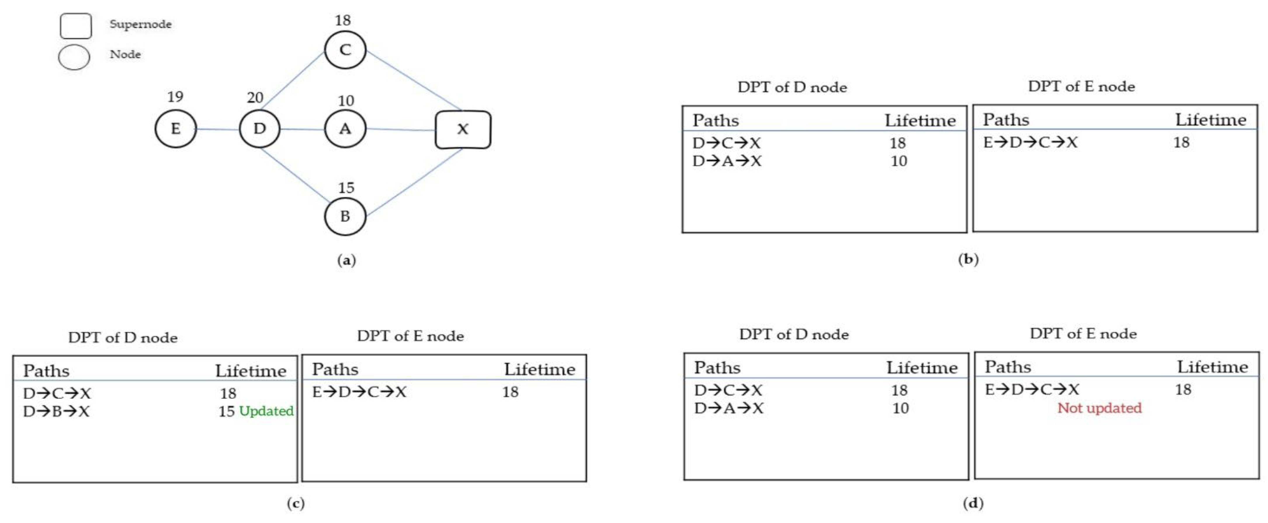
In DPV, ADPV, and MPD, each node that updates the DPT, receiving a new disjoint path or a disjoint path of a higher lifetime, sends the pathinfo message across the network. Consequently, the transmission of control messages persists until no further updates are observed. KDPMS has been refined through the identification and prevention of message transmissions that do not effectuate updates in the disjoint path tables (DPTs) of neighboring nodes, resulting in fewer control messages.
Given the disjoint nature of paths related to the neighbors of each node, the node is constrained to occupy, solely, one of its neighbor’s paths. It is imperative that this particular path possesses the maximum lifetime. Consequently, the transmission of a path characterized by a shorter lifetime would be ineffective in updating the DPT of the adjacent node.
Exemplifying this, node D possesses two disjoint paths to supernode X, and node E maintains a single disjoint path (
Figure 3b). Node B’s transmission of the pathinfo control message updates node D (
Figure 3c), yet node D’s transmission of the pathinfo message fails to update node E due to the latter’s pre-existing path containing node D with a superior lifetime (
Figure 3d). Precluding the transmission of such messages avoids increased message complexity at the source node and computational complexity at the destination node. Consequently, the preservation of the maximum lifetime among paths in segment i (Maxpl
i) is ensured, and potential paths capable of updating Maxpl
i are communicated via pathinfo messages.
Following the completion of pathinfo messages, DPT and MDPT with m + m′ segments are established. Subsequently, Algorithm 2 is executed at each node for connectivity construction, the identification of required neighbors, and clustering in KDPMS. The segments in the DPT are arranged based on the lifetimes, adhering to the condition ∀i (lifetime (DPTi) > lifetime (DPTi+1)). Concurrently, MDPT updates itself in alignment with DPT, maintaining ∀i (MDPTi.d = DPTi.d).
A requisite condition for achieving k-disjoint paths to m-supernode connectivity is that k ≥ m. To connect each node to m-supernodes, the proposed algorithm selects the first k − m + 1 paths of the first segment (DPT1, 1…k−m+1) to connect to the primary supernode, and the first paths of segments 2 to m (DPT2…m,1) to connect to the secondary supernode. For example, for k = 3 and m = 2, two paths of segment one are selected for connecting to the primary supernode, and one path of segment two is selected for linking to the secondary supernode. This yields k-disjoint paths to m-supernode connectivity, prioritizing paths with the longest lifetime from each node to the designated supernodes. Once the disjoint paths have been determined, each node identifies the first node of the selected paths (without considering itself) as its required neighbors and readjusts its transmission power to connect to its remotest neighbor. Subsequently, it communicates this neighborhood update to its neighbors via a Notify message.
In KDPMS, clustering is utilized to confine supernode movement and balance sensor node energy consumption. Designating each supernode as a cluster head, nodes join the cluster of a supernode within DPT
1.d. This straightforward clustering method optimally distributes network load, as each node possesses paths with the longest lifetime to the primary supernode. Subsequently, a notification message (comprising ID, node residual energy, DPT
1, and MDPT
1) is transmitted to the primary supernode, signaling membership. This data exchange mitigates data delay and the number of control messages during supernode movement, as explained in
Section 3.5.
| Algorithm 2 Finding required neighbors, sensor clustering, and connectivity-centric topology design |
Input: DPT, m, m′, k
Output: RN
RN ← 0
If |DPT| ≥ m + m′
Sort (DPT)
DPT ← {DPTi | i ≤ m + m′}
End if
S ← {DPT1, 1…k−m+1 ∪ DPT2…m,1}
For all p ∈ S
RN ← RN ∪ p. first
End for
For all p ∈ RN
Transmit notify(p) // Notify to required neighbors
End for
Notify (DPT1.d, DPTi, MDPTi, RE) // Notify to cluster head |
Theorem 1. The number of control messages in KDPMS is nearly equal to half of the messages sent by the DPV and ADPV.
Proof. In accordance with references [
5,
6], the message complexity for a node in both DPV and ADPV is expressed as O(
nΔ), where
n represents the node count and Δ signifies the maximum degree of a node. Within the framework of KDPMS, the guarantee to preserve the maximum lifetime within segment
i, denoted as Maxpl
i, is firmly established. The transmission of potential paths capable of updating Maxpl
i is facilitated through the exchange of pathinfo messages. It is imperative to emphasize that a path with a superior lifetime possesses the ability to update Maxpl
i. In the best-case, the initial path in DPT
i boasts the highest path lifetime. Consequently, subsequent paths received by the node lack the capacity to update Maxpl
i. In this context, the node’s control message transmissions amount to 1. Conversely, in a worst-case scenario, the first path in DPT
i features the lowest path lifetime, with subsequent paths arranged in ascending order of path lifetime in DPT
i. Each received path in this scenario triggers a Maxpl
i update, leading to the transmission of control messages. Given that the node’s degree is represented as Δ, the number of messages transmitted in this circumstance equals Δ. On average, the number of transmitted messages in KDPMS is denoted as
, which is nearly equal to half of the messages sent by the DPV and ADPV. □
Theorem 2. The message complexity of path information collection and connectivity-centric topology design in KDPM is O(nΔ), and the runtime equals O(nΔ2).
Proof. According to [
5,
6], a node’s message complexity is O(
nΔ), with
n denoting the number of nodes and Δ representing the maximum degree of the node. While KDPMS enhancements result in a reduction in the transmitted control messages, the message’s complexity remains unaffected.
Upon receiving the pathinfo message, a node combines the received and existing paths in LPT
i, sorting them by path lifetime.
K-disjoint paths are allocated to DPT
i, and the next
k′ paths are assigned to MDPTi. Each node then identifies required neighbors and a primary supernode. The union operation complexity is O(
p), path sorting is O(
p logp), selecting
k +
k′ disjoint paths (Algorithm A1) is O (
) [
5,
6], identifying the required neighbors is O(
k), and determining the primary supernode is O(1). This results in a computational complexity of O
), where
p signifies the number of joined paths in LPT
i. Given that each node transmits O(
nΔ) messages, it follows that each node receives O(
nΔ
2) messages. Consequently, the overall asymptotic running time for each node is expressed as O
. Given that
k,
k′, and
p are constants, the time complexity is thereby established as O(
nΔ
2). □
3.3. Node Failure Tolerance in KDPMS (the First Layer’s Fault Tolerance)
Once node failure leads to
k-disjoint paths to
m-supernode disconnectivity, the
node failure message, containing the failed node’s ID, is sent by the neighbors of the failed node along the network. Upon receiving the message, each node checks all the paths in the DPT and MDPT, removing the path containing the failed node. Given the disjoint nature of paths in DPT and MDPT, each node failure causing
k-vertex disconnectivity removes only one path. Therefore, the KDPMS algorithm ensures that it can restore
k-disjoint paths to
m-supernode connectivity if there is a path in the MDPT. Algorithm 3 represents the pseudocode of this subroutine, with the notations shown in
Table 1.
| Algorithm 3 Node failure tolerance algorithm in KDPMS |
Input: k, k′, DPT, MDPT
Output: DPT, MDPT
Failednode ← 0
For all received node failure δ do
If δ.failednode ∈ DPT1
If δ.failednode ∈ DPT1,1…k−m+1
DPT1← DPT1 − p | {p ∩ δ.failednode ≠ 0}
LPT1 ← DPT1 ⋃ MDPT1
Update path lifetime (LPT1)
Sort (LPT1)
DPT1 ← {pi ∈ LPT1 | i ≤ k}
MDPT1 ← {pi ∈ LPT1 | i > k}
Execute Algorithm 2
Else
DPT1 ← DPT1 − p | {p ∩ δ.failednode ≠ 0}
LPT1 ← DPT1 ⋃ MDPT1
Sort (LPT1)
DPT1 ← {pi ∈ LPT1 | i ≤ k}
MDPT1 ← {pi ∈ LPT1 | i > k}
Endif
Endif
Foreach (i > 1 && i ≤ m) // Failed node in segments 2 to m
If δ.failednode ∈ DPTi,1
DPTi ← DPTi − p | {p ∩ δ.failednode ≠ 0}
LPTi ← DPTi ⋃ MDPTi
Update path lifetime (LPTi)
Sort (LPTi)
DPTi ← {pj ∈ LPTi | j ≤ k}
MDPTi ← {pj ∈ LPTi | j > k}
Execute Algorithm 2
Else
DPTi ← DPTi − p | {p ∩ δ.failednode ≠ 0}
LPTi ← DPTi ⋃ MDPTi
Sort (LPTi)
DPTi ← {pj ∈ LPTi | j ≤ k}
MDPTi ← {pj ∈ LPTi | j > k}
Endif
Endfor
Foreach (i > m && i ≤ m + m′) // Failed node in segments m + 1 to m + m′
If δ.failednode ∈ DPTi
DPTi← DPTi − p | {p ∩ δ.failednode ≠ 0}
LPTi ← DPTi ⋃ MDPTi
Sort (LPTi)
DPTi ← {pj ∈ LPTi | j ≤ k}
MDPTi ← {pj ∈ LPTi | j > k}
Endif
Endfor
Foreach (i ≥ 1 && i ≤ m + m′) // Failed node in MDPT
If δ.failednode ∉ DPTi && δ.failednode ∈ MDPTi
MDPTi ← MDPTi − p | {p ∩ δ.failednode ≠ 0}
Endif
Endfor
Transmit (δ.failednode)
Endfor |
To elucidate this algorithm and its impact on connectivity restoration, we elaborate its effects on node l. Nodes are connected through k-disjoint paths to m-supernodes (in DPT1, 1…k−m+1 and DPT2…m,1). KDPMS ensures k-vertex disconnectivity if a failed node is present in these paths. Subsequently, the path with the failed node in DPTi is eliminated (where i denotes the segment of the node failure occurrence). After merging the remaining k − 1 paths in DPTi with MDPTi, path lifetimes are updated per (A7), and the updated paths are sorted by lifetime. The initial k paths are assigned to DPTi, and the remaining paths are assigned to MDPTi. Paths are updated via update lifetime messages from origin to destination and backward lifetime information from nodes in the path. Upon restoring k-vertex connectivity, a path shifts from MDPTi to DPTi, and the list of the required neighbors of the node is changed. Consequently, the node adjusts its transmission power to reach the farthest neighbor based on the updated list. The number of nodes in k paths is kλ, leading to a k-vertex disconnectivity probability of , where is the number of active sensor nodes in the network.
If the failed node is not in the subset of k-disjoint paths but is found in DPT1…m+m′, the failed node’s path is removed from DPTi. The remaining DPTi paths are then merged with MDPTi paths and reorganized. The initial k paths are reinstated in DPTi, and the remaining paths are allocated to MDPTi. As k-vertex disconnectivity does not occur in this case, path lifetimes remain unaltered to minimize the control message overhead. It should be noted that the following failed nodes update these paths. If the failed node exclusively exists in MDPTi, the path containing the failed node is eliminated, reducing the count of maintenance disjoint paths by 1. Ultimately, the node failure message is transmitted to neighboring nodes within the network.
Theorem 3. The number of paths eliminated from each node’s DPT and MDPT after node failure i is as follows: Theorem 4. The number of node failures resulting in path elimination and subsequently leading to k-vertex disconnectivity, is as follows: Theorem 5. The number of update lifetime messages of each node upon failed node i is Theorem 6. The message complexity of node failure tolerance in KDPMS is O(Δ2).
Proof. In the event of a node failure causing k-vertex disconnectivity, update lifetime messages are dispatched for k + k′ paths in DPTi and MDPTi. Given that k + k′ < Δ, the message complexity for k-vertex connectivity restoration is bounded by O(Δ). In the worst-case scenario, where paths are disjoint, the number of connectivity restorations is O(Δ), resulting in a message complexity of O(Δ2) for each node. □
3.4. Supernode Failure Tolerance in KDPMS (the Second Layer’s Fault Tolerance)
The transmission of the supernode failure message occurs through the neighboring nodes of the failed supernode in the network, and is triggered when it leads to k-vertex to m-supernode disconnectivity. Upon the reception of this message, a node activates the supernode failure tolerance algorithm. It is worth noting that the DPT comprises m + m′ segments, each corresponding to a required supernode. Paths to the primary supernode, secondary supernodes, and alternative supernodes are stored in DPT1, DPT2…m, and DPTm+1…m+m′, respectively. The failure of a supernode in DPT1…m results in both m-supernode and k-vertex disconnectivity. This is attributed to the fact that the k-disjoint paths, those with the longest lifetime, are connected to supernodes 1 to m. Additionally, the failure of the primary supernode in a node leads to the disconnection of the node from the cluster head. The details of KDPMS’s various and valuable scenarios for handling the supernode failure message are detailed below.
In the case of a failed supernode in DPT
1 (the primary supernode), the elimination of all paths in both DPT
1 and MDPT
1 is performed, resulting in the disconnection of this node from the cluster head. Subsequently, the shift operation
is executed, during which the DPT and MDPT segments replace the previous segments. The shift operation is defined as follows:
As the DPT1 and MDPT1 paths have changed, their union is classified, updating the lifetimes of the paths by sending an update lifetime message. Then, the paths are arranged based on their lifetimes, placing the first k paths in DPT1 and the remaining paths within MDPT1. Then, the node sends a notification to new supernode DPT1.d (containing the ID, residual energy, DPT1, and MDPT1) so that supernode d can consider it a cluster member. This is known as a cluster head change. Finally, this node executes Algorithm 2 to update its required neighbors and leads to k-vertex to m-supernode connectivity by adjusting transmission power.
Should a supernode failure be situated in DPT2…m, it results in k-vertex to m-supernode disconnectivity due to the presence of paths to the secondary supernodes within these segments. In such instances, is activated, with i denoting the segment corresponding to the failed supernode. Subsequently, the node executes Algorithm 2 to update required neighbors, thereby restoring k-vertex to m-supernode connectivity. In this case, the update lifetime message is not sent to avoid an increased number of control messages.
In the event of a supernode failure within DPT
m+1…m+m′, there is no
k-vertex to
m-supernode disconnectivity as these segments pertain to alternative supernodes. In this scenario, only the execution of
is required to eliminate the failed supernode from the list of alternative supernodes. Subsequently, each node communicates the supernode failure message to its neighbors. The pseudocode for the supernode failure tolerance algorithm is delineated in Algorithm 4.
| Algorithm 4 Supernode failure tolerance algorithm in KDPMS |
Input: k, k′
Output: DPT, MDPT
Failedsupernode ← 0
For all received supernode failure δ do
If δ.failedsupernode ∈ DPT1.d // primary supernode failure
Eliminate DPT1, MDPT1
For each i < m + m′
DPTi ← DPTi+1
MDPTi ← MDPTi+1
Endfor
LPT1 ← DPT1 ⋃ MDPT1
Update path lifetime (LPT1)
Sort (LPT1)
DPT1 ← {pi ∈ LPT1 | i ≤ k}
MDPT1 ← {pi ∈ LPT1 | i>k}
Execute Algorithm 2
Endif
If δ.failedsupernode ∈ DPT2…m.d // secondary supernode failure
i ← S(DPT.d) // Finding the segment corresponding to the failed supernode
Eliminate DPTi, MDPTi
For each l > i && l < m + m′
DPTl ← DPTl+1
MDPTl ← MDPTl+1
Endfor
LPTi ← DPTi ⋃ MDPTi
Sort (LPTi)
DPTi ← {pj ∈ LPTi | j ≤ k}
MDPTi ← {pj ∈ LPTi | j > k}
Execute Algorithm 2
Endif
If δ.failedsupernode ∈ DPTm+1…m+ m′.d // alternative supernode failure
i ← S (DPT.d)
Eliminate DPTi, MDPTi
For each l > i && l < m + m′
DPTl ← DPTl+1
MDPTl ← MDPTl+1
Endfor
Endif
End for |
Theorem 7. The number of paths eliminated from each node’s DPT and MDPT after supernode failure i and node failure j is Theorem 8. The number of update lifetime messages upon failed supernode i and failed node j is as follows: Theorem 9. The message complexity of supernode failure tolerance in KDPMS is O(Δ).
Proof. When supernode failure occurs in DPT1, an update lifetime message is sent for the k + k′ paths in DPT1 and MDPT1. Since k + k′ < Δ, message complexity in each m-supernode connectivity restoration is O(Δ). Given that each node has m + m′ segments, there are m + m′ restorations in the worst scenario. Thus, asymptotic message complexity is O(Δ (m + m′)). Since m and m′ are constants, message complexity is O(Δ). □
3.5. Supernode Mobility Model in KDPMS
In Algorithm 5 of KDPMS, clusters established through the application of Algorithm 2 are utilized. In this clustering method, each node belongs to the DPT
1.d cluster, and the number of clusters corresponds to the number of supernodes. It is important to highlight that a supernode failure would decrease the cluster count by 1. Given that DPT
1 has only one supernode, KDPMS guarantees that each node is a member of a single cluster. Consequently, a graph of sensor nodes is formed within each supernode. With an assumed uniform distribution of nodes in the clusters, the number of nodes in each cluster equals
, where
n is the number of sensor nodes and
ns is the number of supernodes.
| Algorithm 5 Determining migration points in KDPMS |
Input: N
Output: S
S ← 0
← N
is not empty
S ← S ⋃ MaxDegree()
← − S − { x| x ∈ neighbor(S) }
end while |
This phase aims to identify optimal migration points for distributing relay tasks within each cluster, a task known to be NP-hard [
27]. This paper addresses this challenge by adapting the optimization algorithm based on the dominating set problem, achieving a complexity of O(n
2). The goal of this algorithm is to identify a set of points, denoted as S, with the smallest cardinality such that every node is either in S or has a neighbor in S. It is essential to highlight that supernodes execute this distributed algorithm, ensuring it does not impact the computational complexity of individual nodes. The outcome is a minimal subset of sensor nodes, serving as the mounting points for the mobile supernode in each deployment. Following the identification of migration points within each cluster, the
migration point node message is transmitted to all nodes within these subsets. This ensures that, in the event of a supernode failure causing the disconnection of these nodes from the cluster head, the subsequent primary supernode is promptly notified about the migration points.
The relocation of each supernode to the new migration point induces a topological change, leading to
k-vertex to
m-mobile supernode disconnectivity. In a previous study [
28], all nodes in the network sent an
Init message, and
k-disjoint paths were extracted from each node to others, ensuring
k-vertex connectivity at each migration point. However, approach [
28] suffered from control message overhead and the requirement for substantial memory to store these paths. In our current research, upon identifying S for each cluster, S members transmit the
Init message to the network. Cluster members receive the message and execute Algorithm 1 to extract disjoint paths to the sender, conserving memory by storing these paths in the supernode. Subsequently, when the supernode migrates to a new point, it dispatches paths to its member nodes through a
path-update message.
An additional mobility challenge lies in determining the next migration point to avert relay node failure and maintain a balanced traffic distribution. To accommodate the adaptation of mobile supernodes to nodes’ residual energy, the migration point subset for mobile supernodes is organized according to the residual energy within each supernode. The node with the highest residual energy is chosen as the subsequent migration point, aiming to prolong the network’s lifetime. The duration of the supernode’s migration or stay at each migration point is computed based on the energy levels of neighboring nodes [
18]. Consequently, when the residual energy of neighboring nodes falls below a specified threshold, the supernode initiates migration to the next point.
Theorem 10. The message complexity of KDPMS equals O(nΔ), and the runtime equals O(nΔ2).
Proof. In [
52], it was proven that the maximum cardinality
γ(
G) in the minimum dominating problem was 3
n/8 or O(
n). Due to the disjoint nature of paths among neighboring nodes, each node can send a maximum of Δ messages. Therefore, the message complexity of the mobility model is equal to O(
nΔ). The number of
node failure tolerance messages sent is O(Δ
2), the number of
supernode failure tolerance messages sent is O(Δ), and the number of
path information collection messages sent is O(
nΔ). As a result, the total asymptotic message complexity of each node is O(
nΔ + Δ
2 + Δ +
nΔ). Therefore, the message complexity of each node is O(
nΔ). Given that each node sends O(
nΔ) messages, it can be concluded that each node receives O(
nΔ
2) messages. Based on Theorem 2, the computational complexity of each received message is O(
) = O(1). As a result, the computational complexity of KDPMS is O(
nΔ
2). □
4. Results and Discussion
This section evaluates the proposed algorithm against DPV and ADPV algorithms using manual simulation. The simulator operates on stochastic topologies, calculating and reporting various parameters. The results suggest that nodes and supernodes are uniformly distributed in a 600 m × 600 m area, with an initial maximum transmission range (R
max) of 100m for nodes and supernodes, as indicated in [
5,
6]. Experiments cover node counts from 100 to 550, with
k values of 2, 3, and 4,
m values of 2, 3, and 4, and supernode ratios of 3% and 5%. Each experiment runs the mentioned algorithms 100 times, reporting their average rates.
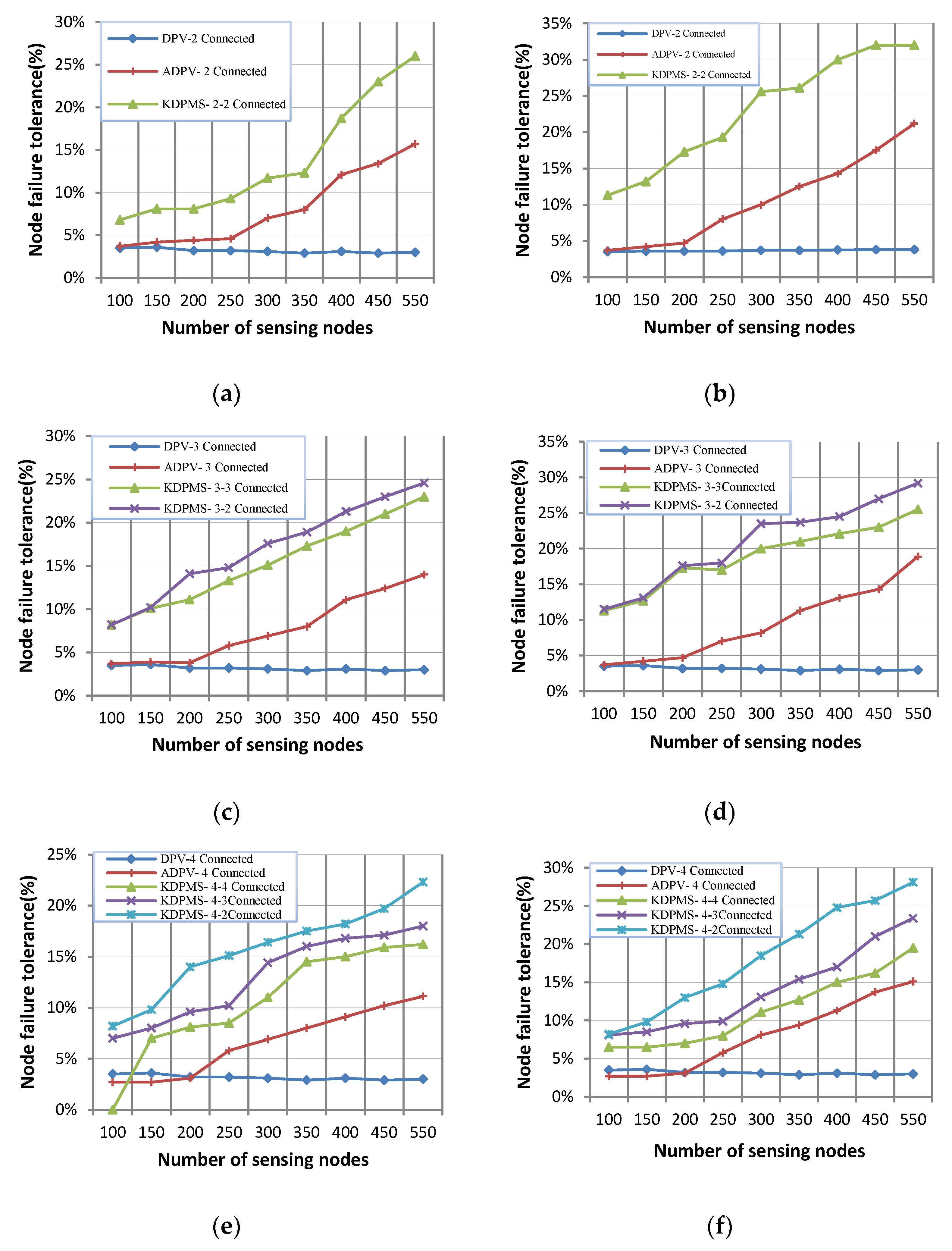
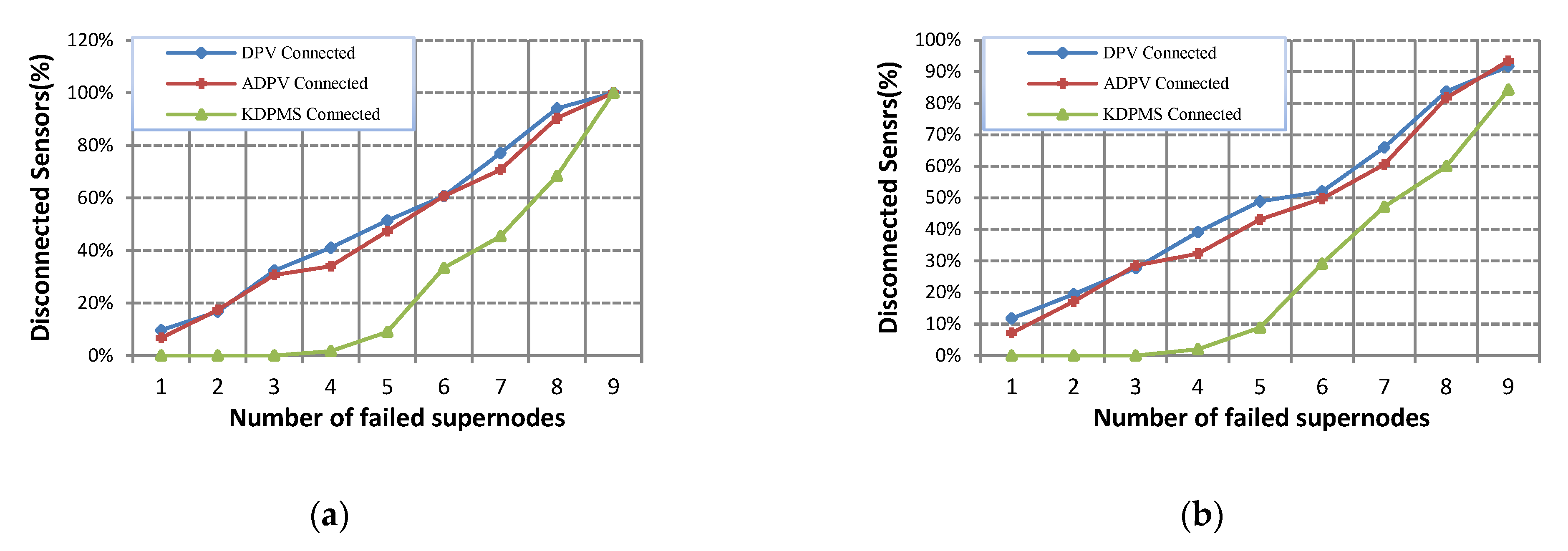
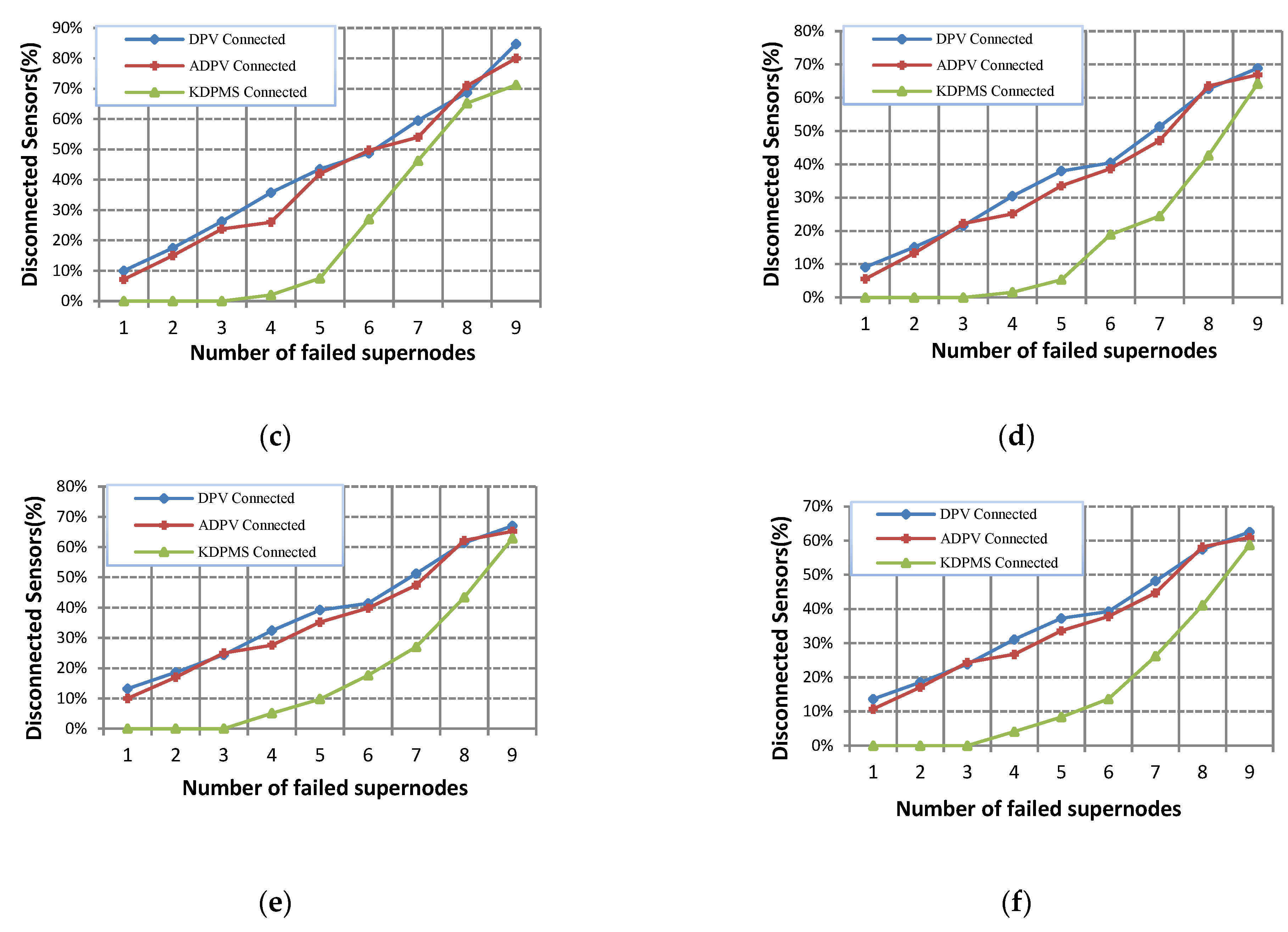
Figure 4 and
Figure 5 depict the node fault tolerance in ADPV, DPV, and KDPMS algorithms. Two modes of supernode disconnectivity and
k-disjoint paths to
m-supernode disconnectivity are considered for a more precise assessment of this evaluation. Supernode disconnectivity occurs when at least one active node exists in the network connecting to no supernode. The disconnectivity of
k-disjoint paths to
m-mobile supernodes occurs when a node exists in a network, and the number of its disjoint paths for access to
m-mobile supernodes is less than
k, or the number of supernodes available for connectivity is less than
m. According to this definition,
Figure 4 shows the percentage of node failure tolerance before supernode disconnectivity, and
Figure 5 depicts the percentage of node failure tolerance before
k-disjoint paths to
m-mobile supernode disconnectivity.
According to the simulation results, the KDPMS algorithm outperforms ADPV and DPV within two modes of supernode connectivity maintenance and
k-disjoint paths to
m-supernode connectivity.
Figure 4 and
Figure 5 show that the DPV algorithm cannot be considered a suitable solution for fault tolerance due to the stationary and damping status of nodes near the supernode. Relay node damping leads to the disconnectivity of many nodes from supernodes, and this algorithm does not provide a mechanism to overcome this problem. Regarding energy awareness and retrieval paths, the ADPV algorithm provides higher node fault tolerance than DPV does. ADPV outperforms dense networks compared to sparse ones because more supernodes exist in these networks, and more disjoint paths are available for connectivity. These figures show no significant difference between ADPV and DPV in sparse networks. Moreover, the damping status of nodes near the supernode is the main shortcoming of ADPV, like DPV, which results in the disconnectivity of other nodes from the supernode set.
In DPV and ADPV, supernode disconnectivity happens when 5% and 23% of nodes fail, respectively. K-vertex disconnectivity occurs after node failures of 2% and 8%. On the other hand, k-vertex disconnectivity and supernode disconnectivity occur from node failures of 16% and 58%, respectively, in the KDPMS algorithm. In sparse networks of 100, 150, and 200 nodes, the average node failure tolerance for k-vertex connectivity and supernode connectivity is, respectively, 3% and 5% in the DPV and 4% and 14% in the ADPV. In contrast these values are 10% and 48% in the KDPMS algorithm.
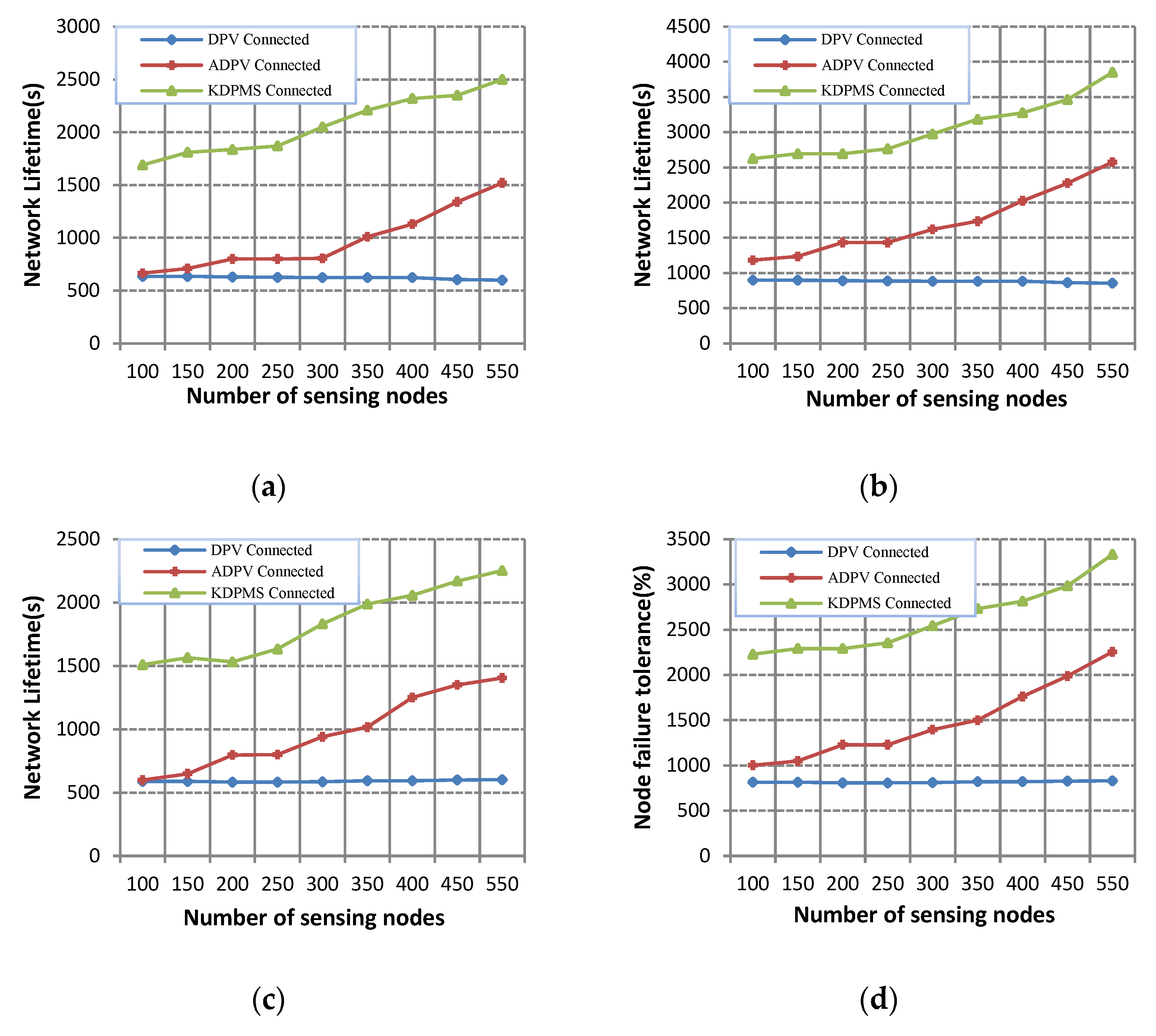
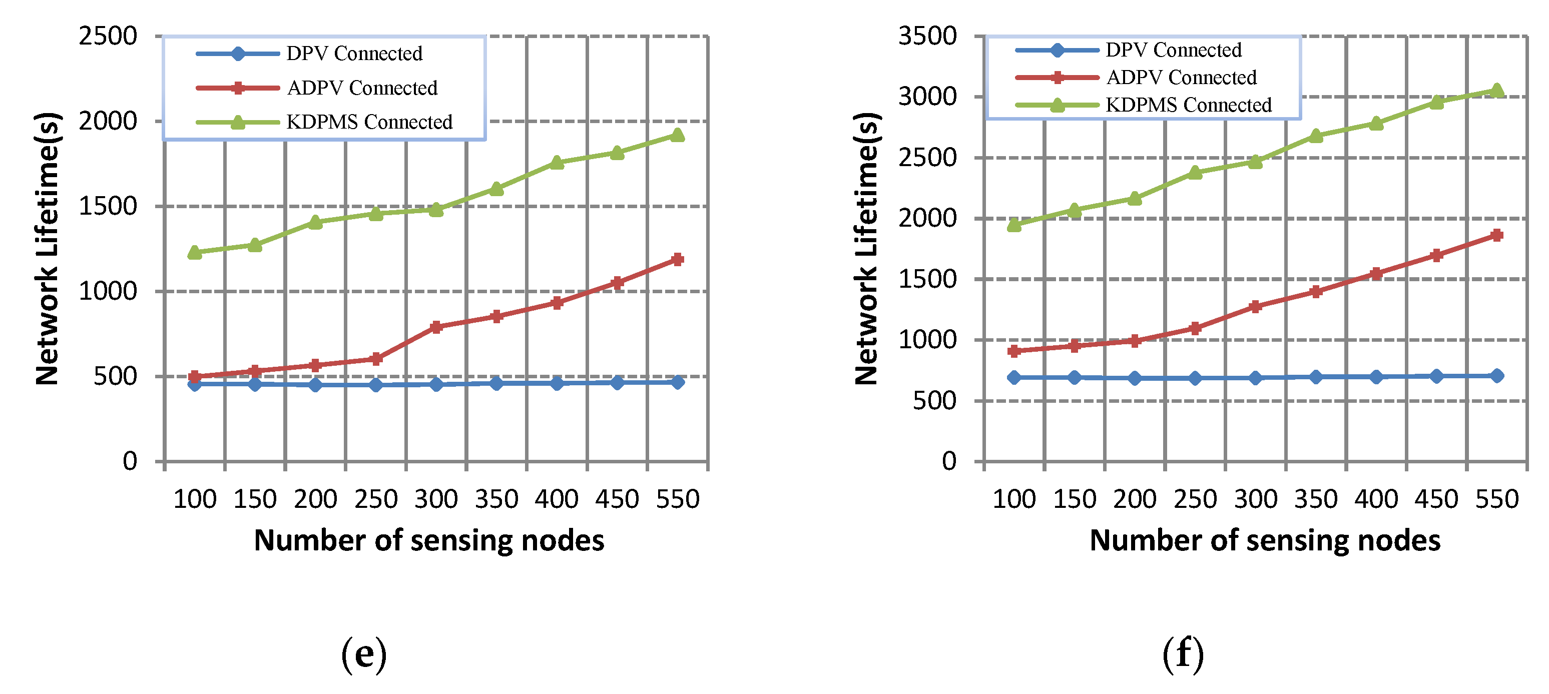
Figure 6 and
Figure 7 depict the network lifetime for instances depicted in
Figure 4 and
Figure 5. The network lifetime for the DPV algorithm is not significantly affected by network density, as relay node damping disconnects other nodes from the network, reducing the network’s lifetime. Regarding the energy awareness in the ADPV algorithm, the energy depletion of relay nodes is carried out more slowly than it is under DPV, resulting in a longer lifetime of this algorithm. Also, ADPV has a longer lifetime in dense networks than in sparse ones because more disjoint paths are extracted in dense networks. In addition to the nodes’ energy considered for extracting and retrieving disjoint paths in the KDPMS algorithm, mobile supernodes are used to solve the challenge of damping relay nodes. As seen in
Figure 6 and
Figure 7, this algorithm has a longer lifetime than that under previous techniques.
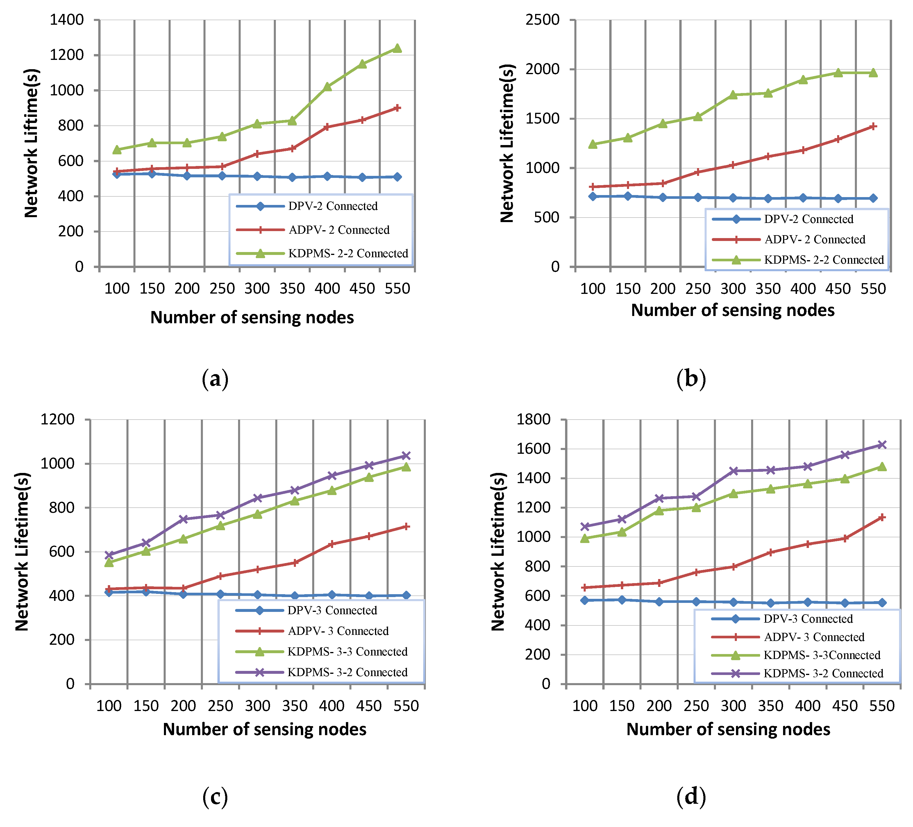
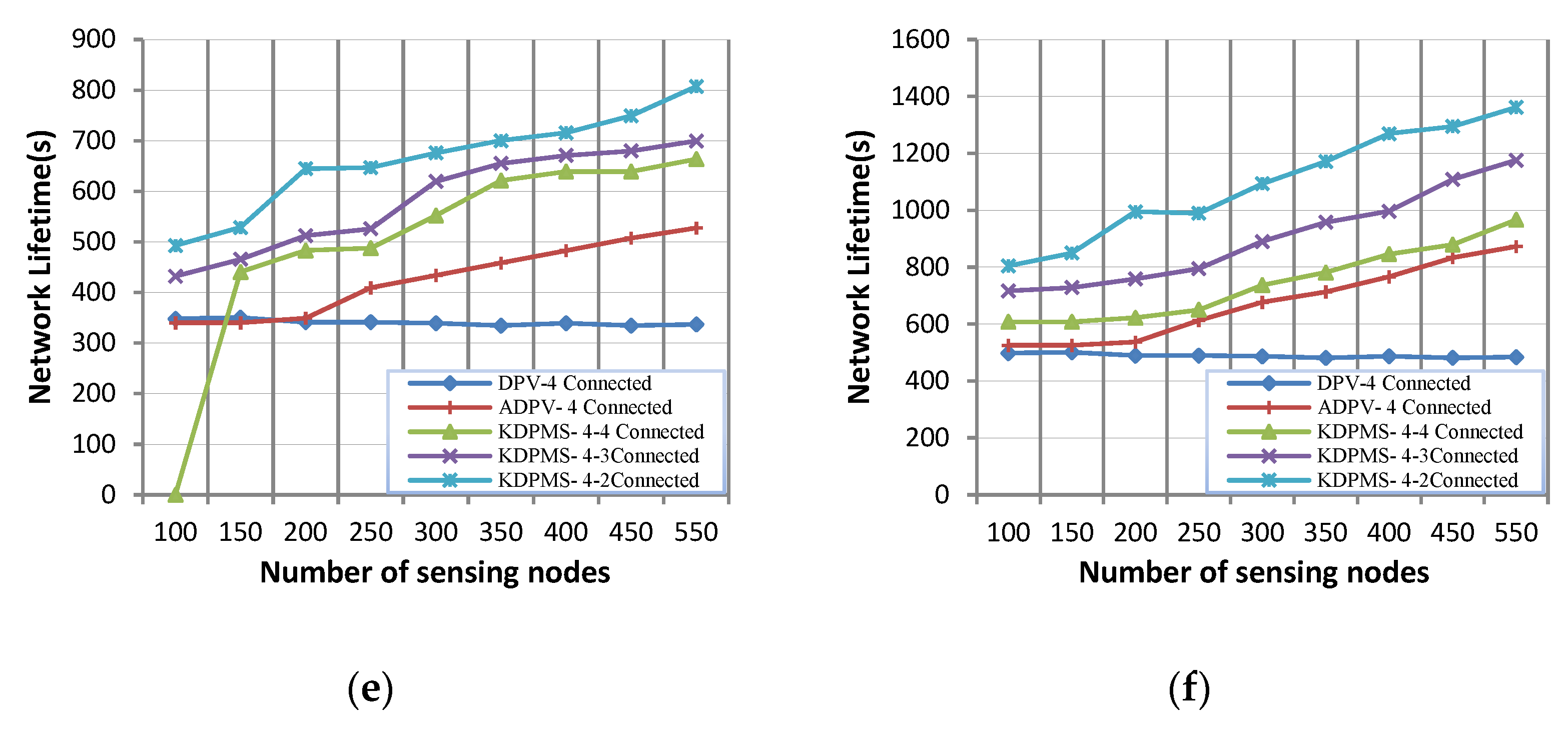
These data show that the KDPMS algorithm outperforms DPV and ADPV in terms of lifetime in supernode and k-vertex connectivity. Within 2-vertex, 3-vertex, 4-vertex, and 1-vertex supernode connectivity, respectively, the lifetime of this method is, on average, 107%, 123%, 79%, and 235% higher than that of the DPV algorithm. On the other hand, in the cases of 2-vertex, 3-vertex, 4-vertex, and 1-vertex supernode connectivity, respectively, the lifetime of this algorithm is 46%, 56%, 35%, and 88% higher than that of the ADPV algorithm.
Based on the results obtained, an increased k value leads to a higher node transmission range and a shorter network lifetime. Additionally, an Sr increase leads to a longer lifetime of the network. The strength of KDPMS is seen in k-vertex to m-mobile supernode connectivity. In this case, when supernode disconnectivity occurs, another supernode is retrieved for reconnection, and when k-vertex disconnectivity happens, another path of MDPT is retrieved for k-vertex connectivity. Therefore, this algorithm has a longer lifetime compared to that of the previous algorithm. For instance, in the case of k = 4 and sr = 3% and 550 nodes, the lifetime of KDPMS-4-2 connectivity equals 807 s, while it equals 527 s in ADPV-4 connectivity.
The supernode fault tolerance for the DPV, ADPV, and KDPMS algorithms is shown in
Figure 8. Many nodes are disconnected from the network with each supernode failure because DPV and ADPV do not offer a solution for supernode fault tolerance. Each node in the KDPMS algorithm is connected to
m supernodes, and
m′ alternative supernodes are used to retrieve
m-supernode connectivity. Examples of
Figure 8 have been assessed using the assumptions that
k = 2,
sr = 3%,
m = 2, and
m′ = 2.
It is assumed in all experiments in
Figure 8 that nodes are disconnected from the network only due to the failure of supernodes, while ignoring node failure in these experiments. As is seen in
n = 300, the first supernode failure causes a disconnectivity of 9.4% and 6.6% of nodes from the network in DPV and ADPV. The reason is that these nodes available in the generated topology are only connected to the failed supernode. This limitation hinders their effective strategy for supernode failure tolerance. In the KDPMS algorithm, no considerable disconnectivity occurs in the network up to the third supernode failure because two alternative supernodes exist for connectivity retrieval. The number of nodes’ disconnectivity dramatically increases after the
m +
m′ supernode failure. Therefore, unlike the previous techniques that do not have supernode fault tolerance, this algorithm provides an appropriate tolerance up to the
m +
m′ supernode failure level. On average, the percent of disconnected nodes before the failure of the
m +
m′ supernode equals 36% and 42% in ADPV and DPV algorithms, respectively, while it equals 2% in the KDPMS algorithm.
Figure 9 shows connectivity retrievals of ADPV and KDPMS algorithms for
k = 2, 3, and 4, and
sr = 3%. Connectivity retrieval occurs in the ADPV when a node failure leads to
k-vertex disconnectivity. Therefore, an increase in the
k number leads to an increase in connectivity retrievals. In dense networks with many nodes, an increase in node failure leads to an increase in the number of connectivity retrievals in ADPV. In addition to node failure, supernode failure and mobility result in connectivity retrieval in the KDPMS algorithm.
In this algorithm, as k increases, the disconnectivity of the k-vertex increases, necessitating more connectivity retrieval. Additionally, more nodes mean more instances of node failure and connectivity retrievals. Regarding the proposed technique’s supernode failure tolerance, more supernodes imply more supernode failures and also more requirements for connectivity retrieval. Additionally, supernode mobility and connectivity retrieval increase as the number of supernodes increases. For k = 2, 3, and 4, the connection retrievals in KDPMS are 4.9, 5.9, and 7.7 times higher than these rates in ADPV.
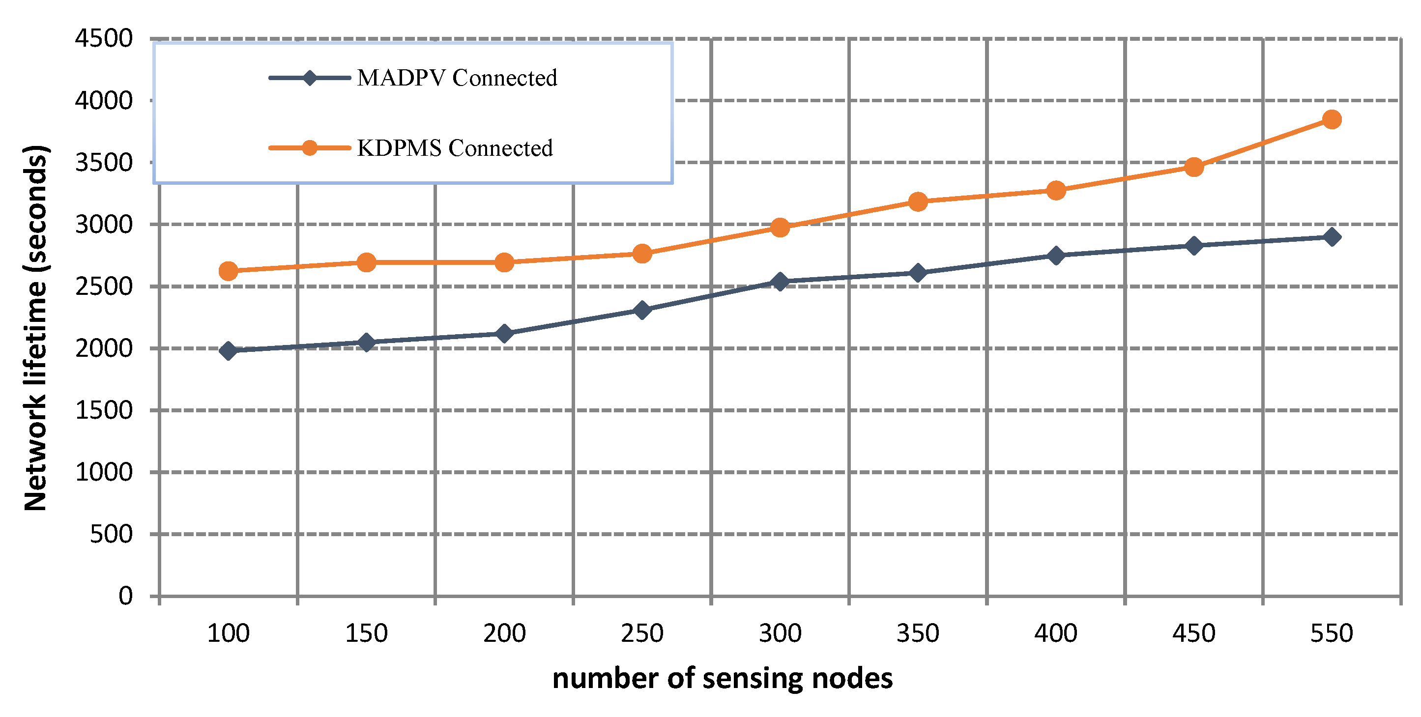
For a better and more accurate evaluation of the suggested technique and a comparison with fault tolerance solutions that use mobile supernodes, ADPV has been developed, enabling it to use mobile supernodes (MADPV). Each supernode moves to the next random migration point when the stay time has expired according to the fully stochastic movement pattern of KDPMS. The network lifetime and the total number of control message transmissions are compared in this examination. The total number of control messages in KDPMS and MADPV for k = 2 and sr = 5% is shown in
Figure 10.
According to the first observation, an increase in the number of sensor nodes and supernodes causes a rise in the mobility of supernodes and a corresponding increase in the number of message exchanges required for connectivity retrieval. The second observation demonstrates that the MADPV method offers more message exchanges than the suggested technique does since it needs some message exchange for each supernode’s mobility towards the new migration point to create a k-vertex topology, while the proposed method maintains k-vertex connectivity during migration. On average, the number of control messages transmitted in the proposed algorithm is 22% less than that under MADPV.
Figure 11 depicts the network lifetime for
k = 2 and
sr = 5% in KDPMS and MADPV algorithms. The first observation indicates that increasing the number of nodes and supernodes would increase the network lifetime due to the extraction of more disjoint paths. The second observation shows that the MADPV algorithm’s high number of control messages can reduce network lifetime by increasing node energy usage. The third observation shows that stochastic mobility in MADPV has prevented the covering of all relay nodes and the early death of these nodes would reduce the network’s lifetime. On average, the network lifetime of the proposed technique is 43% greater than that of MADPV.


