Conveyor-Belt Dryers with Tangential Flow for Food Drying: Mathematical Modeling and Design Guidelines for Final Moisture Content Higher Than the Critical Value

Abstract

The mathematical modeling presented in this work concerns the conveyor-belt dryer with the tangential flow of air with respect to food. This dryer, if operating in co-current, has the advantage of well preserving the organoleptic and nutritional qualities of the dried product. In fact, it has a low air temperature in the final stretch where the product has low moisture content and is therefore more temperature sensitive. It is a bulkier dryer than the continuous through-circulation conveyor dryer with a perforated belt. The latter is therefore more frequently used and has received greater study attention from researchers and designers of the industry. With the aim to propose guidelines for a rational design of the conveyor-belt dryer with tangential flow, a mathematical model was developed here through the differentiation of the drying rate equation followed by its integration performed along the dryer belt. Consequently, and with the assumption that the final moisture content X_F of the product is higher than the critical moisture content X_C, the relationships between the intensive quantities (temperatures, humidity and enthalpies), the extensive quantities (air and product flow rates) and the dimensional ones (length and width of the belt), were obtained. Finally, on the basis of these relationships, the rules for an optimized design for X_F > X_C were obtained and experimentally evaluated.

1. Introduction

The drying of food products aims to reduce the activity of water [1,2] and therefore to increase the shelf life of the product, without resorting to the more expensive refrigeration or freezing processes, and to contain storage and transportation costs for the reduction of weight and volume [3,4,5,6].

The lowering of the water content in solid food products must be carried out by evaporating the water contained in the product, exposing it to a stream of hot and dry air. All this inside a plant called a dryer.

Drying brings the product to relatively high temperatures [7,8] with negative effects on the quality of the dried product. Then, denaturation of proteins, loss of vitamins, etc., are possible. However, from the thermodynamics of the air it is known that during the removal of the water the product takes on a lower temperature than the drying air, in particular a value equal to or close to the wet bulb temperature. Therefore, the damage in many cases is limited and the drying operation remains highly interesting.

The fundamental problem of drying is the mathematical modeling of the thermo-hygrometric exchange processes between the air and the wet product [9,10]. The differential equations of the heat and mass transfer must be set and resolved in closed form [11,12,13] or by numerical methods. Over the course of several decades, the scientific literature has produced solutions of these differential equations, and therefore many simulations and experimental tests, with reference to a multitude of products [14,15,16,17,18,19,20,21,22,23,24,25,26,27,28,29,30,31,32,33,34,35,36,37,38,39,40,41,42,43,44,45,46,47,48,49,50,51,52,53].

A second problem that arises is the mathematical modeling of the operation of the dryers and therefore the definition of guidelines for their design.

From the dawn of agriculture, humanity has learned that it is possible to carry out the drying of agricultural products simply by posing them on surfaces lapped by the environmental air, if only it is hot and dry. This simple first drying way is still in use today, one thinks of the drying of tomatoes, seedless grapes, apricots, plums, figs, cod, hay, etc.

Its main characteristic is that the air mass of the environment is infinitely greater than the product placed in drying. Therefore, the drying air is able to maintain constant both its temperature T_A and its specific humidity x.

With elementary dryers of this type, called solar dryers, made with surfaces exposed to environmental air, the design guidelines are very simple and are reduced to the calculation of the drying time.

A second drying way refers instead to the use of preheated air sent with fans to touch the product according to a flow inside a closing carter. There are several dryers that refer to this continuous operation scheme, namely: the through-circulation conveyor-belt, tangential flow conveyor-belt, tunnel trucks, rotary, fluid bed and the pneumatic [54,55]. All are characterized not only by the movement of hot air forced by the fans, but also by the movement of the product. Compared to the product, the air can have a tangential flow in counter-current or co-current or a cross flow (through-circulation conveyor dryers). Further differences between the dryers are in the feed system of the food products, but all the dryers internally present variations in the thermodynamic parameters of the drying air, and therefore the mathematical modeling of the operation and design results more complex.

Finally, a third drying way provides preheated and forced air to pass through a mass of static product. This is the case with silo dryers. The crossing requires that the product be presented in granular or fibrous form so that the air passes through it regularly, creating a more intimate thermo-hygrometric exchange. The mathematical description of the operation of these silo dryers is also complex due to the discontinuous process. In fact, the product evolves its moisture content both over time and in the space, as well as the air, what requires the setting of partial differential equations.

Below we will deal with conveyor-belt dryers. The characteristic element of this type of dryer is the belt on whose surface the food product to be dried is distributed. The conveyor belt moves inside a tunnel where hot drying air circulates.

As can be seen from Figure 1 and Figure 2, two solutions are possible. In the first solution, the air passes through the product and then goes to the top of the tunnel. This is possible due to the presence of a perforated belt (through-circulation conveyor-belt dryer). In this case, the drying air is blown starting from the area below the belt (Figure 1).

In the second solution, the air flows tangentially over the product, as the conveyor belt has not perforated (conveyor-belt dryer with tangential flow). The drying air therefore circulates only in the volume above the belt, entering at one end and exiting at the opposite one (Figure 2).

The perforated belt dryer with crossing air from below or from the top was analyzed very thoroughly. In fact, various mathematical models are available [56,57,58,59,60,61,62] which hypothesize the drying air which uniformly crosses the entire length of the dryer with a constant air inlet temperature.

The conveyor-belt dryer with tangential flow (Figure 2), on the other hand, has the air channeled, what results in continuously changing its characteristics of temperature T_A and specific humidity x, in the length of the dryer. Therefore, the mathematical description of the thermo-hygrometric exchange between the air and the product is complicated precisely because of these variabilities. Below, a mathematical model will be developed to determine the average flow rate of evaporated water G_EV of the dryer and then to design it when the output product is still with a moisture content higher than the critical moisture content (X_F > X_C).

2. Materials and Methods

2.1. Preliminaries

The drying rate can be defined [55] as:

$$R=-\frac{dX}{dt}=\frac{G_{EV}}{m_D}$$

(1)

where: R (s⁻¹) is the drying rate; X = m_W/m_D (kg/kg) is the moisture content (dry basis) of the product without dimensions; m_W is the mass of water and m_D is the dry mass; G_EV = dm_W/dt is the flow rate of evaporated water (kg/s).

By applying an enthalpy balance [55] we obtain:

$$G_{EV}=\frac{q}{r}=\frac{\alpha ·A·\left(T_A-T_{WB}\right)}{r}$$

(2)

where: q (W) is the heat transfer rate from the air to the product; T_A (K) is the air temperature; T_WB (K) is the wet bulb temperature of the air. It is also the temperature of the food product if it has a moisture content X greater than the critical one X_C. In other words, if the product is moist enough to behave like pure water; α (Wm⁻¹K⁻¹) is the convection coefficient; A (m²) is the area of the product lapped by the air; r (J/kg) should be the latent heat of the water vapor at the wet bulb temperature T_WB, but it assumes a greater value as indicated by [55].

By inserting (2) in (1), we obtain:

$$R=\frac{\alpha ·A·\left(T_A-T_{WB}\right)}{r·m_D}$$

(3)

This equation indicates that, with X > X_C, T_WB is constant and if the air temperature T_A also remains constant, then the drying rate R becomes constant and is called R_C.

With the constant rate R_C, the (1) can be rewritten:

$$R_C=-\frac{dX}{dt}=\frac{\Delta X}{t_C}$$

(4)

where: $\Delta X=\left(X_F-X_I\right)$, X_I is the initial moisture content and X_F è is the final moisture content of the period at constant speed. Therefore, the drying time t_C at a constant rate is:

$$t_C=\frac{\left(X_I-X_F\right)}{R_C}$$

(5)

This is the situation that occurs with the first drying way (solar dryer), that is, with constant T_A and with X_F > X_C.

However, when the moisture content of the product X falls below the critical moisture content X_C, the water runs out on the surface of the product. This does not prevent drying since water from the inside comes by diffusion through the internal mass. However, the process is conditioned precisely by the reduced speed of water diffusion towards the surface. Therefore, the balance between the heat transfer rate q, from the hot air to the product, and the heat transfer rate q that accompanies the flow rate of evaporated water G_EV from the product to the air [55], occurs with a product temperature T_P higher than that of the wet bulb T_WB. Equation (2) is still valid provided that the temperature T_P replaces the T_WB, which confirms the reduction of G_EV and therefore also of the drying rate R.

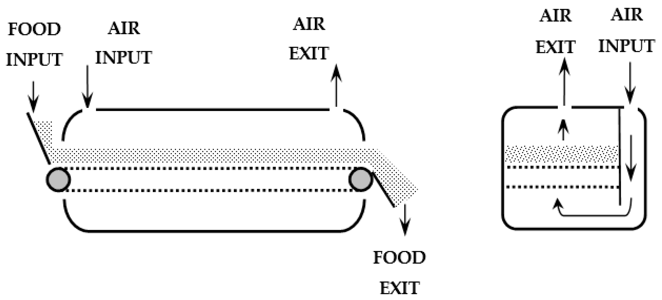
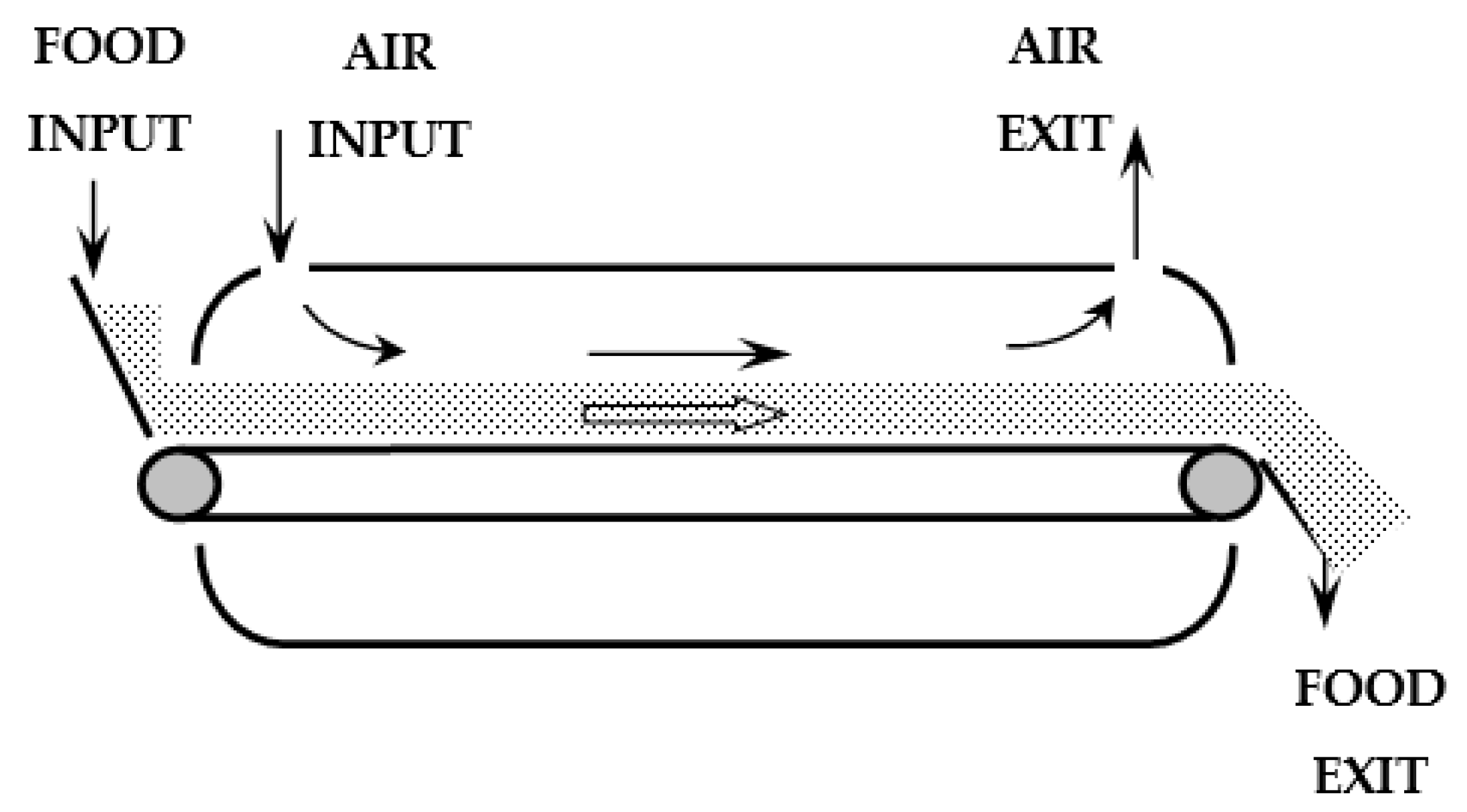
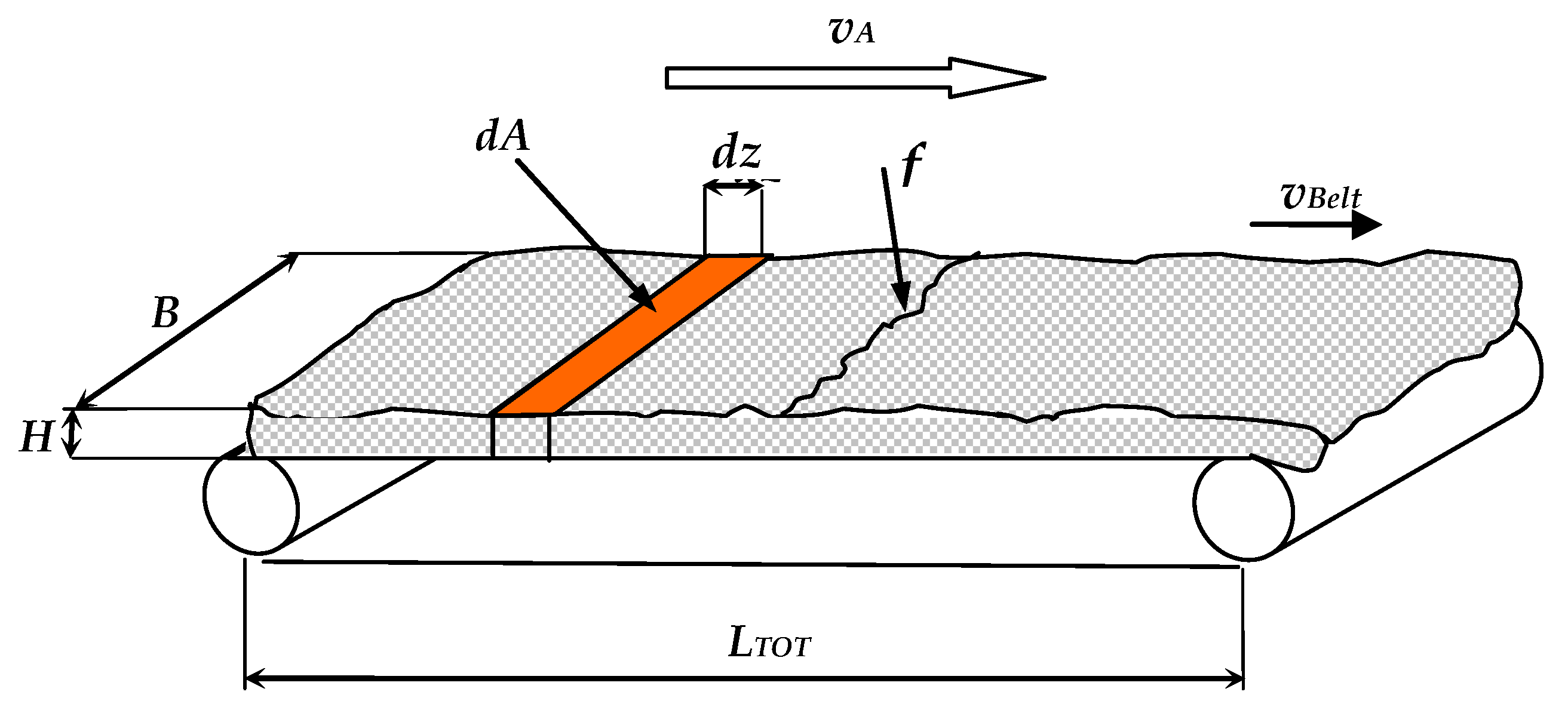
2.2. Mathematcal Modeling of the Conveyor-Belt Dryer with Tangential Flow

In the introduction, a second drying mode was defined. It refers to the use of preheated air sent with fans to touch the product according to a flow inside a top closing carter. Among the various types of dryers, the conveyor-belt dryer with tangential flow (Figure 2) will be discussed below.

In this case, the temperature of the drying air decreases in the length of the dryer, from the inlet to the outlet, and therefore it is necessary to write the Equation (2) in differential form:

$$d{G}_{EV}=\frac{dq}{r}=\frac{\alpha ·dA·\left(T_A-T_{WB}\right)}{r}$$

(6)

To develop a mathematical model suitable for determining the overall flow rate of the evaporated water G_EV in the entire dryer, it is necessary to proceed with the integration of (6). This requires knowledge of the mathematical relationship between the air temperature T_A and the coordinate along which the dryer belt develops.

The mathematical model will be developed under the condition X_F > X_C, that is the output product is still with a moisture content higher than the critical one. This means that the product maintains its T_P temperature constant and equal to that of the wet bulb of the T_WB air throughout the dryer.

Figure 3 shows the scheme of a belt dryer completed by the diagram of the temperatures of the T_A air and the T_P product.

The infinitesimal heat transfer rate dq in (6) is transferred from the air to the product through the elementary area dA (Figure 3):

$$dq=\alpha ·dA·\left(T_A-T_{WB}\right)$$

(7)

where: α is the convection coefficient; dA is the elementary area; T_A is the air temperature when it comes into contact with the dA area; T_P = T_WB is the temperature of the product, assumed equal to that of the wet bulb of the air.

Under the condition that the drying process is adiabatic, i.e., that it takes place in the absence of heat dispersion through the walls, then the elementary heat transfer rate dq can also be written in relation to the elementary variation of temperature dT_A of the air (in its dry component). In fact, it undergoes a decrease by flowing over the elementary area dA, as it warms to the same area dA (Figure 3):

$$dq=-G_A·c_A·d{T}_A$$

(8)

where: G_A is the mass flow rate of dry air; c_A is the specific heat of dry air; dA is the elementary area; dT_A is the elementary decrease in air temperature when it laps the dA area. The negative sign appears to make the heat transfer rate dq positive since dT_A is negative.

Figure 3 shows that, from the beginning of the dryer, the temperature of the product, T_PI, was considered equal to the wet bulb T_WB. This is an acceptable approximation because, in the enthalpy balance of the dryer [55], the thermal energy required to heat the dry component of the product, from T_PI to T_WB, is less than 1% of the total thermal energy supplied by the hot air. While the thermal energy necessary to heat the water contained in the product from T_PI to T_WB is approximately 3% and will be taken into consideration during the development of the mathematical model.

By equating (7) with (8), we obtain: $\alpha ·dA·\left(T_A-T_{WB}\right)=-G_A·c_A·d{T}_A$; from which, by separating the variables A and T_A and moving on to integration, we have:

$$\frac{\alpha }{G_A·c_A}·\underset{0}{\overset{A_{TOT}}{{\displaystyle \int }}}dA=\underset{T_{AE}}{\overset{T_{AI}}{{\displaystyle \int }}}\frac{d{T}_A}{\left(T_A-T_{WB}\right)}$$

(9)

where: A_TOT is the total area of the product surface inside the dryer; and T_AI and T_AE are the dryer input and exit air temperatures (Figure 3). The result of the integration is:

$$\frac{\alpha }{G_A·c_A}·A_{TOT}=\ln \left(\frac{T_{AI}-T_{WB}}{T_{AE}-T_{WB}}\right)$$

(10)

Setting, as shown in Figure 3, $T_{AI}-T_{WB}=\Delta T_a$ and $T_{AE}-T_{WB}=\Delta T_b$, then moving the logarithmic term to the left and the product G_A·c_A to the right, and multiplying both members by $T_{AI}-T_{AE}$, we have:

$$\alpha ·A_{TOT}\frac{\left(T_{AI}-T_{AE}\right)}{\ln \left(\frac{\Delta T_a}{\Delta T_b}\right)}=G_A·c_A\left(T_{AI}-T_{AE}\right)$$

(11)

The right term:

$$G_A·c_A\left(T_{AI}-T_{AE}\right)=q$$

(12)

is precisely the heat transfer rate q released to the product from the drying air throughout the length of the dryer due to the cooling effect from T_AI to T_AE. Having admitted that it goes completely to the product without dispersion to the outside, then the left term of (11) becomes the heat exchange equation between the air and the product. Just add and subtract the T_WB temperature inside the parenthesis, to have $\left(T_{AI}-T_{AE}\right)=\left(\left(T_{AI}-T_{WB}\right)-\left(T_{AE}-T_{WB}\right)\right)=\Delta T_a-\Delta T_b$. Definitely:

$$q=\alpha ·A_{TOT}\frac{\left(\Delta T_a-\Delta T_b\right)}{\ln \left(\frac{\Delta T_a}{\Delta T_b}\right)}=\alpha ·A_{TOT}·\Delta T_{mL}$$

(13)

As is known [63] the quantity: $\frac{\left(\Delta T_a-\Delta T_b\right)}{\ln \left(\frac{\Delta T_a}{\Delta T_b}\right)}$ is defined as the logarithmic mean temperature difference between the air and the product: $\Delta T_{mL}$.

Here, the total flow rate of evaporated water G_EV from the product bed within the tunnel of the dryer is:

$$G_{EV}=\frac{q}{r}=\frac{\alpha ·A_{TOT}}{r}·\Delta T_{mL}$$

(14)

where: r is the thermal energy to produce 1 kg of superheated steam at the temperature of the T_A air as we will see in Section 3.1.6.

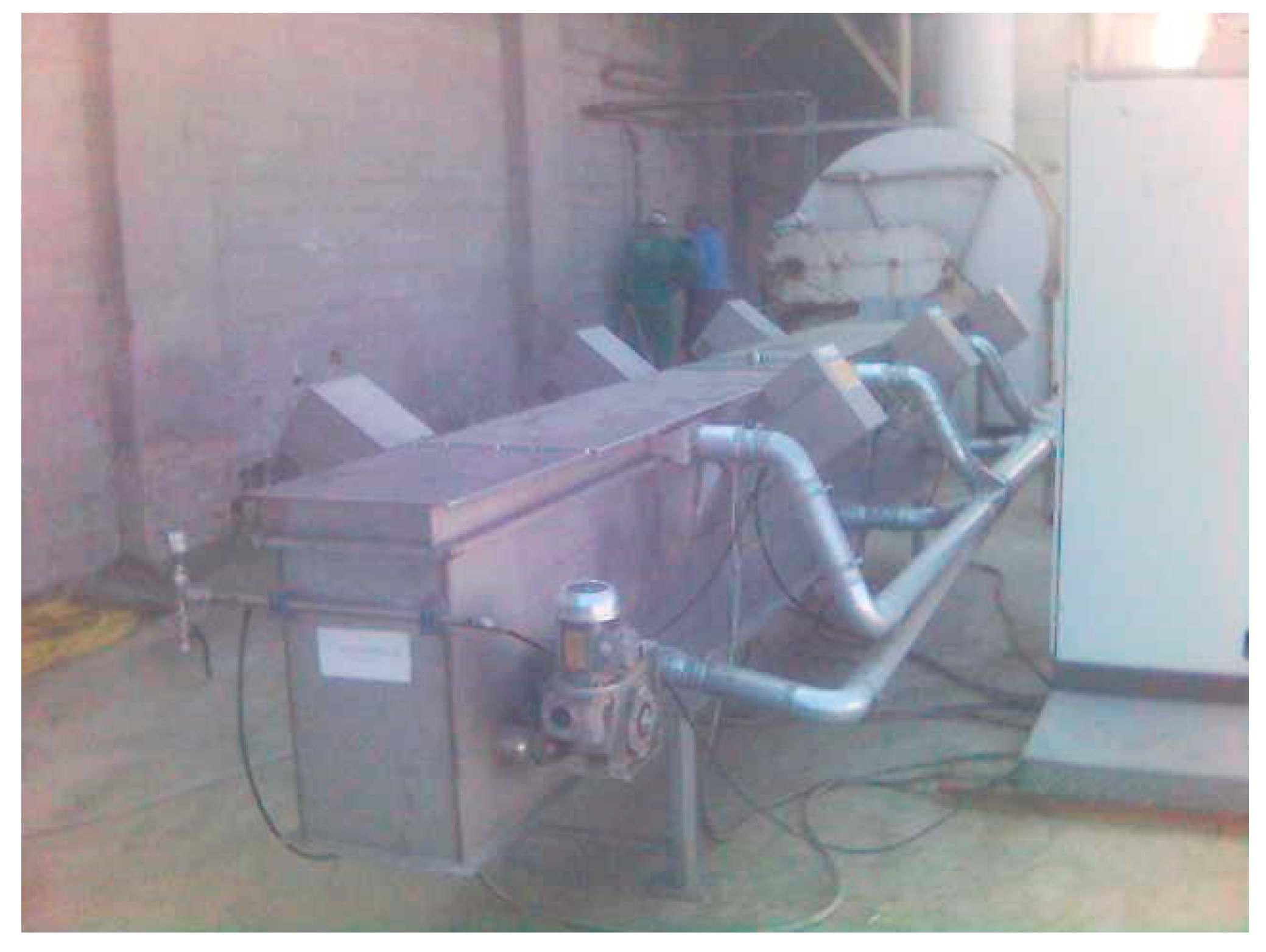
2.3. Experimental Equipment

A pilot dryer consisting of a non-perforated belt, B_I = 0.3 m wide and L_TOT = 6 m long, was used (Figure 4). The scheme of its operation was the same as in Figure 3. The dryer was fed with alfalfa distributed on the belt for a height (H_I) of 0.05 m. The geometric and operational characteristics are shown in

Table 1. Geometrical and operational data of the pilot dryer.

Quantity	Symbol	Value
Belt width	BI (m)	0.3
Belt length	LTOT (m)	6.0
Belt speed	vBelt (m/s)	0.005
Air input velocity	vAI (m/s)	2.6
Air section	AA (m2)	0.15
Air input volumetric flow rate	QAI (m3/s)	0.395
Air input temperature	TAI (K)	393
Air input density	ρAI (kg/m3)	0.896
Air mass flow rate	GAI (kg/s)	0.354
Alfalfa input moisture content (D.B.)	Xl	1.892 ± 0.110
Alfalfa input moisture content (W.B.)	YI (%)	65.4 ± 1.3
Alfalfa input bulk density	ρBulkI (kg/m3)	197 ± 7.5

.

Five PT100 resistance thermometers were installed along the air flow channel: one at the air inlet and the others following one every 1.5 m; therefore, the last probe was on the exit of the dryer. Consequently, the air temperatures were measured and registered in a data logger. The alfalfa temperature at the input and exit of the dryer was measured with an infrared thermometer. Each test was replicated 5 times.

The moisture content of alfalfa was measured in the laboratory by weighing before and after drying in a stove at 408 K (135 °C) for 2 h respectively. Each test was replicated 5 times. The bulk density was obtained by measuring the mass and volume of the samples.

3. Results

3.1. Design Guideline Conveyor-Belt Dryer with Tangential Flow for Food with X_F > X_C

The two previous Equations (12) and (14) are useful for designing a conveyor-belt dryer with tangential flow. Below we analyze the various quantities to identify what will be the starting data of the design problem and the unknowns to be obtained.

3.1.1. Input and Exit Temperatures of the Drying Air

The air temperatures, at the input T_AI and at the exit T_AE of the dryer, must be defined in order to calculate the logarithmic mean temperature difference in ΔT_mL. The input temperature must be established according to the characteristics of the product to be dried. It may be greater, the smaller and more uniform the size of the product, and the more permeable the surface of the product and the more humid the entering product are. All these facts allow to keep the product sufficiently humid on the surface and therefore its temperature equal to the wet bulb. Furthermore, it is necessary to avoid denaturing some components of the product. For example, and with reference to the grain, the maximum recommended T_AI for maize is 115–120 °C, while oilseeds, such as soy, can be subjected to a T_AI temperature of no more than 90 °C. For rice, it must be below 70 °C. For herbaceous products, due to the size of the leaves and the stems, as well as to the high permeability of the surfaces, the T_AI can reach 500 °C [64] and, if very humid, even 800 °C [65].

Regarding the air exit temperature T_AE, it must be adequately higher than that of the wet bulb T_WB. In fact, even if the product were pure water, this temperature T_WB would be reached by the air at the end of a continuous dryer only if it had infinite length (Figure 3).

Therefore, in order to have not too long dryers, the next Equation (23) indicates that we must keep the logarithmic mean temperature difference ΔT_mL, between the air and the product, high enough. As is known, it is assumed here that the product is throughout the dryer with a moisture content higher than the critical value, and therefore, at a temperature equal to that of the wet bulb T_WB. In order to have good values of the logarithmic mean temperature difference: $\Delta T_{mL} \frac{\left(\Delta T_a-\Delta T_b\right)}{\ln \left(\frac{\Delta T_a}{\Delta T_b}\right)}$, both ΔT_a and ΔT_b must be high; as shown in Figure 3, the latter is high if the temperature of the air at the exit of the dryer T_AE is also high.

As a rule of thumb, T_AE is set a few tens of degrees higher than that of the exit product. For example, with a T_AI of 120 °C, the T_WB, provided by the psychrometric diagram, is 34 °C and therefore the final temperature of the T_AE air can be set between 50 °C and 60 °C.

3.1.2. Flow Rate of Evaporated Water and Final Moisture Content

The flow rate of the evaporated water G_EV must be considered a datum of the problem. It is related to the flow rate of the product to be dried G_I, the input moisture content X_I and the final moisture content X_F to be reached during the process. Indeed, the manufacturers identify the performance of the dryers, in their production range, precisely through the flow rate of evaporated water expressed in kg/h.

The evaporated water flow rate is the difference in the initial water mass m_WI of the product and the final one m_WF, divided by the time interval Δt required for this evaporation: $G_{EV}=\frac{m_{WI}-m_{WF}}{\Delta t}$. The total mass of wet product (dry mass m_D plus water mass m_WI) that enters the dryer in this time interval Δt is the flow rate of the wet product, i.e., at the conditions of input into the dryer: $G_I=\frac{m_D+m_{WI}}{\Delta t}$.

By dividing the flow rate of the evaporated water by the flow rate of the wet product $\frac{G_{EV}}{G_I}$, we obtain: $\frac{G_{EV}}{G_I}=\frac{m_{WI}-m_{WF}}{m_D+m_{WI}}$. Dividing above and below by the dry mass m_D and defining the moisture content on a dry basis $X=\frac{m_W}{m_D}$, we have: $\frac{G_{EV}}{G_I}=\frac{X_I-X_F}{1+X_I}$.

Therefore, given the three quantities mentioned above X_I, X_F and G_I, relating to the wet product and its drying process, the determination of G_EV, as the initial datum of the problem, is immediate:

$$G_{EV}=G_I\frac{X_I-X_F}{1+X_I}$$

(15)

3.1.3. Wet Product Flow Rate

The mass flow rate of the wet product at the input of the dryer G_I can be defined as the volumetric flow rate of the bulk wet product Q_BulkI multiplied by the bulk density of the wet product at the input of the dryer, ρ_BulkI: $G_I={\rho }_{BulkI}·Q_{BulkI}$.

It is convenient to highlight the volumetric flow rate Q_BulkI since it is equal to the initial section multiplied by the feed speed of the product, equal to the belt speed v_Belt: $Q_{BulkI}=B_I\cdot H_I\cdot v_{Belt}$. It is therefore very easy to control Q_BulkI both by adjusting the initial height of the bulk product H_I (B_I is the initial width) with a toothed roller and by adjusting the speed of advancement of the belt v_Belt. Therefore:

$$G_I=B_I·H_I·v_{Belt}·{\rho }_{BulkI}$$

(16)

Finally, by inserting (16) in (15) we have:

$$G_{EV}=B_I·H_I·v_{Belt}·{\rho }_{BulkI}\frac{X_I-X_F}{1+X_I}$$

(17)

3.1.4. Area of the Product Lapped by the Air

The total area of the product, A_TOT, exposed to the drying air, can be imagined as the length, L_TOT, of the belt of the dryer multiplied by a transverse dimension f (Figure 5):

$$A_{TOT}=f·L_{TOT}$$

(18)

The quantity f is an unknown and it is difficult to predict, therefore it will have to be determined experimentally as we will see in the subsequent Section 3.1.9.

3.1.5. Convection Coefficient

The convection coefficient α depends on the velocity of the drying air v_A, in addition to other parameters. We can proceed to the calculation of α through the formulas between the dimensionless numbers of Nusselt, Reynolds and Prandtl Nu = f (Re, Pr) [55,66].

However, for greater precision, we can proceed experimentally as we will see in the subsequent Section 3.1.9.

3.1.6. Thermal Energy r

The thermal energy r to produce 1 kg of superheated steam at the air temperature T_A is equal to the difference in enthalpy [55] of the superheated steam at T_A and that of the water contained in the product to be dried at the temperature T_PI:

$$r=c_W\left(T_{WB}-T_{PI}\right)+{\lambda }_{WB}+c_{SV}\left(T_A-T_{WB}\right)$$

(19)

where: c_W is the water specific heat capacity equal to 4.187 kJ kg⁻¹K⁻¹; λ_WB is the latent heat at the wet bulb temperature T_WB; c_SV is the superheated steam specific heat capacity equal to 1.92 kJ kg⁻¹K⁻¹.

Using hot air in the dryer with temperatures T_A between 343 K (70 °C) and 423 K (150 °C) and considering an initial product temperature T_PI of 293 K (20 °C), the thermal energy r assumes a value between 2542 and 2694 kJ kg⁻¹. If an arithmetic mean value r of 2617 kJ kg⁻¹ is assumed, a standard error of 1.6% and a maximum error of 2.9% are verified. These errors must be accepted as a consequence of the imposition r = constant. Otherwise, the mathematical modeling developed in the previous Section 2.2 would have been much more complicated and consequently the design guidelines would become impractical.

3.1.7. Flow Rate of Drying Air

Having admitted as negligible both the thermal dispersion from the walls of the dryer and the thermal energy of preheating the dry mass of the product, the heat transfer rate q is used for preheating, evaporating and overheating up to T_A the flow rate of the water G_EV contained in the product, so that the moisture content drops from X_I to X_F. For this reason, this heat transfer rate q will be related to the G_EV given by Equation (17) and to the thermal heat r provided by Equation (19):

$$q=G_{EV}·r=B_I·H_I·v_{Belt}·{\rho }_{BulkI}\frac{X_I-X_F}{1+X_I}·r$$

(20)

This heat transfer rate q is provided by the incoming hot air in the dryer with the flow rate G_A, i.e., by Equation (12). By equating (12) with (20), we can finally derive the flow rate of drying air G_A:

$$G_A=\frac{B_I·H_I·v_{Belt}·{\rho }_{BulkI}}{c_A·\left(T_{AI}-T_{AE}\right)}·\frac{X_I-X_F}{1+X_I}·r$$

(21)

3.1.8. Length of the Dryer

By combining Equations (14), (17) and (18), we obtain:

$$L_{TOT}=\frac{B_I·H_I·v_{Belt}·{\rho }_{BulkI}·r}{\alpha ·f·\Delta T_{mL}}·\frac{X_I-X_F}{\left(1+X_I\right)}$$

(22)

It is convenient to collect the quantities B_I, H_I and f in a single parameter that could be called a form factor, $F=\frac{f}{B_I·H_I}$:

$$L_{TOT}=\frac{v_{Belt}·{\rho }_{BulkI}·r}{F·\alpha ·\Delta T_{mL}}·\frac{X_I-X_F}{\left(1+X_I\right)}$$

(23)

This equation becomes the design equation because it defines the length of the dryer belt, L_TOT, after the values of the dryer belt speed, v_Belt, and the initial moisture content X_I and the final moisture content X_F, were chosen.

Before using the Equation (23), it is necessary to calculate: (1) the value of ΔT_mL as in Section 3.1.1; (2) the value of thermal energy r as in Section 3.1.6; the value of the bulk density of the wet product at the beginning of the dryer ρ_BulkI, with the experimental method as in the next Section 3.1.9; the value of the product, F·α, of the form factor F and of the convection coefficient α, with experimental method as in the next Section 3.1.9.

3.1.9. Experimental Evaluation of F·α

The difficulties of the theoretical evaluation of F and the approximation of the calculation result of α with the monomial relations Nu = f (Re, Pr) [66], due to the complex shape of the objects to be dried, suggest proceeding with the experimental determination of the product F·α. In the laboratory, we prepared a batch dryer with a B_I · H_I product section identical to that of the belt dryer to be designed, but with a short length, L_D. Above the product, high H_I, flows the drying air with the same characteristics and the same flow rate G_A (and speed v_A) as the dryer.

If L_D is short, the exponential decrease in T_A can be approximated with a segment from T_AI to T_AD. Therefore, the average air temperature T_Aa above the product is: $T_{Aa}=\frac{\left(T_{AI}+T_{AD}\right)}{2}$. The heat transfer rate associated with the decrease in air temperature is: $q=c_A·G_A\left(T_{AI}-T_{AD}\right)$. This heat transfer rate must equal that exchanged between the air and the product: $q=\alpha ·A\left(T_{Aa}-T_{WB}\right)$. Since the area of product A lapped by the air is (18) $A=f·L_D$ and remembering that: $F=\frac{f}{B_I·H_I}$, in the absence of thermal loss through the walls and measuring the temperatures T_AI, T_AE and T_WB, we have:

$$F·\alpha =\frac{c_A·G_A·\left(T_{AI}-T_{AD}\right)}{B_I·H_I·L_D·\left(\left(T_{AI}+T_{AD}\right)/2-T_{WB}\right)}$$

(24)

3.1.10. Adjustment of Parameters of the Dryer

If the product keeps the incoming moisture content X_I constant, the dryer, sized with the L_TOT length via Equation (23), will ensure that the product will be dried at the final moisture content X_F expected according to the programmed G_PI flow rate of the wet product.

However, the incoming moisture content can vary, considering that the status of many products depends on the environmental conditions of the previous storage or on the weather conditions, if the products come directly from the field.

Then the same Equation (23) can be used, besides the design equation for the dryer, also as a mathematical modeling to highlight the influence of all the quantities on the final moisture content X_F:

$$X_F=X_I-\left(1+X_I\right)\frac{F·\alpha ·\Delta T_{mL}}{v_{Belt}·{\rho }_{BulkI}·r}·L_{TOT}$$

(25)

Clearly if the incoming moisture content X_I increases, the final X_F increases as well, failing the food safety objective due to the consequent increase in the water activity of the product subsequently stored. Conversely, a decrease in the final moisture content X_F can also occur when X_I decreases, with an unnecessary energy consumption and an increased risk of fire/explosion in the final section of the dryer if the product is dusty. At certain concentrations, the dry dust raised and floating in the drying air can produce explosions from any accidental spark.

In essence, the dryers must be equipped with a feedback system that directly detects the final moisture content of the product X_F, and if this is not the desired one, intervenes accordingly on one of the parameters in Equation (25). For example, the feed speed of the product, through v_Belt, can be varied, decreasing it for example if the X_F is too high, thus leaving the product in the dryer for a longer time.

Alternatively, the inlet temperature of the drying air can be varied. For example, if the final moisture content X_F is still too high, then one can proceed by increasing the inlet temperature of the drying air T_AI. It also follows a partial increase in the exit temperature of the air T_AE. Since the product remains at the temperature of the wet bulb, there is an increase in the logarithmic mean temperature difference between the air and the product, ΔT_mL, which leads to an increase in the heat transfer rate q from the air to the product, intensifying the evaporated water flow rate G_EV. The Equation (25) confirms it.

3.2. Experimental Results

Table 2. Experimental data of the pilot dryer and the batch dryer.

Quantity	Symbol	Value
Air input temperature	TAI ± S.D. (K)	392.2 ± 1.3
Air exit temperature	TAE ± S.D. (K)	331.4 ± 1.2
Air temperature at z = 1.5 m as batch dryer for F·α assessment	TAD ± S.D. (K)	368.8 ± 1.2
Alfalfa input temperature	TPI (K)	310.7 ± 0.6
Alfalfa exit temperature	TPE (K)	311.6 ± 0.9
Log. mean temperature difference	ΔTmL (K)	45.2
Simulated batch dryer length	LD (m)	1.5
Alfalfa final moisture content (D.B.)	XF ± S.D.	0.332 ± 0.016

reports the results of the tests reflecting the mean values of the air temperature T_A and alfalfa T_P ones, together with the relative standard deviation (S.D.), at the input and the exit of the dryer. In addition, the table shows the mean value and the S.D. of the alfalfa moisture content at the input and exit of the dryer. There was no significant difference between the experimental values of the alfalfa temperature T_P and the wet bulb temperature T_WB, quantified with the psychrometric chart.

The T_AI, T_AE e T_P temperatures were used to calculate the logarithmic mean temperature difference ΔT_mL showed in Table 2.

The values of the quantities of Table 2 and some of those of Table 1 were implemented in Equation (23) allowing to calculate the exact value of the quantity F·α:

$$F·\alpha =\frac{v_{Belt}·{\rho }_{BulkI}·r}{L_{TOT}·\Delta T_{mL}}·\frac{X_I-X_F}{\left(1+X_I\right)}=5144 \frac{W}{m^{3}K}$$

(26)

In Section 3.1.9, a simplified equation was proposed to determine the quantity F·α starting from data detectable with a simple test on a batch dryer. To simulate the batch dryer, the pilot dryer belt was stopped and the air temperature T_AD, at distance from input z = 1.5 m, was measured together with the T_AI temperature value, the alfalfa temperature value T_P = T_WB and the length L_D = 1.5 m. This allowed to use Equation (24) which gave an approximate value of F·α equal to:

$$F·\alpha =\frac{c_A·G_A·\left(T_{AI}-T_{AD}\right)}{B_I·H_I·L_D·\left(\frac{\left(T_{AI}+T_{AD}\right)}{2}-T_{WB}\right)}=5248 \frac{W}{m^{3}K}$$

(27)

Comparing this value with the exact value of Equation (26), an error of 2.6% occurs. This is an acceptable error testifying that the procedure proposed in Section 3.1.9 is a valid method.

Figure 6 shows the curve of the air temperature decay, T_A, vs. the distance z from the input of the dryer.

4. Conclusions

Various studies on the mathematical modeling and design guidelines of perforated belt dryer (through-circulation conveyor-belt dryer) are available, while non-perforated belt dryer (conveyor-belt dryer with tangential flow) have been neglected, probably because it is less common.

The co-current version of the conveyor-belt dryer with tangential flow has the advantage of low air temperature in the final stretch where the product has low moisture content. In this condition where the product is in the most temperature-sensitive condition, the fact of being in contact with air less hot, presents itself as a positive aspect of this dryer.

For a greater diffusion of the conveyor belt dryer and therefore for its rational design, a mathematical modeling was carried out in this work. The equations obtained show a decreasing drying rate according to an exponential law, under the condition of the final moisture content of the product higher than the critical one.

Consequently, a series of rational design guidelines were proposed. To validate the mathematical model and the guidelines, especially the Section 3.1.9, experimentation on a pilot dryer was carried out. The results confirmed the validity of the innovative design procedures proposed in this work with an error of 2.6%.

Concerning the last rule of Section 3.1.10, and adjustment of the dryer with the feedback system, the final equation of the mathematical model indicates, for the feedback control chain, the need to start from an instantaneous measurement of the final moisture content of the product. The difficulties of creating a sensor for instantaneous moisture content measurement and the not always acceptable results of hygrometers on the market suggest to study this problem in depth in a future work. A mathematical analysis will have to be done in order to find further relationships between the quantities: in particular, a relationship between the moisture content and a different parameter that is more easily measurable for starting the feed-back control chain.

Finally, it is also necessary to extend the mathematical modeling and the design guidelines for the case of the final product moisture content lower than the critical one (X_F < X_C) in further future work.

References

1. Omolola, A.O.; Jideani, A.I.O.; Kapila, P.F. Quality properties of fruits as affected by drying operation. Crit. Rev. Food Sci. Nutr. 2017, 57, 95–108. [Google Scholar] [CrossRef] [PubMed]
2. Caccavale, P.; De Bonis, M.V.; Ruocco, G. Conjugate heat and mass transfer in drying: A modeling review. J. Food Eng. 2016, 176, 28–35. [Google Scholar] [CrossRef]
3. Fernandes, F.A.N.; Rodrigues, S.; Law, C.L.; Mujumdar, A.S. Drying of exotic tropical fruits: A comprehensive review. Food Bioprocess. Technol. 2011, 4, 163–185. [Google Scholar] [CrossRef]
4. Kaleta, A.; Gornicki, K.; Winiczenko, R.; Chojnacka, A. Evaluation of drying models of apple (var. Ligol) dried in a fluidized bed dryer. Energy Convers. Manag. 2013, 67, 179–185. [Google Scholar] [CrossRef]
5. Marquez, C.A.; de Michelis, A. Comparison of drying kinetics for small fruits with and without particle shrinkage considerations. Food Bioprocess. Technol. 2011, 4, 1212–1218. [Google Scholar] [CrossRef]
6. Tzempelikos, D.A.; Mitrakos, D.; Vouros, A.P.; Bardakas, A.V.; Filios, A.E.; Margaris, D.P. Numerical modeling of heat and mass transfer during convective drying of cylindrical quince slices. J. Food Eng. 2015, 156, 10–21. [Google Scholar] [CrossRef]
7. Bezerra, C.V.; Meller Da Silva, L.H.; Correa, D.F.; Rodrigues, A.M.C. A modeling study for moisture diffusivities and moisture transfer coefficients in drying of passion fruit peel. Int. J. Heat Mass Tran. 2015, 85, 750–755. [Google Scholar] [CrossRef]
8. García-Alvarado, M.A.; Pacheco-Aguirre, F.M.; Ruiz-Lopez, I.I. Analytical solution of simultaneous heat and mass transfer equations during food drying. J. Food Eng. 2014, 142, 39–45. [Google Scholar] [CrossRef]
9. Ertekin, C.; Firat, M.Z. A comprehensive review of thin layer drying models used in agricultural products. Crit. Rev. Food Sci. Nutr. 2017, 57, 701–717. [Google Scholar] [CrossRef]
10. Fernando, W.J.N.; Low, H.C.; Ahmad, A.L. Dependence of the effective diffusion coefficient of moisture with thickness and temperature in convective drying of sliced materials. A study on slices of banana, cassava and pumpkin. J. Food Eng. 2011, 102, 310–316. [Google Scholar] [CrossRef]
11. Friso, D. A Mathematical Solution for Food Thermal Process Design. Appl. Math. Sci. 2015, 9, 255–270. [Google Scholar] [CrossRef]
12. Friso, D.; Baldoin, C. Mathematical Modelling and Experimental Assessment of Agrochemical Drift using a Wind Tunnel. Appl. Math. Sci. 2015, 9, 5451–5463. [Google Scholar] [CrossRef]
13. Friso, D. An Approximate Analytic Solution to a Non-Linear ODE for Air Jet Velocity Decay through Tree Crops Using Piecewise Linear Emulations and Rectangle Functions. Appl. Sci. 2019, 9, 5440. [Google Scholar] [CrossRef] [Green Version]
14. Akdas, S.; Baslar, M. Dehydration and degradation kinetics of bioactive compounds for mandarin slices under vacuum and oven drying conditions. J. Food Process. Preserv. 2015, 39, 1098–1107. [Google Scholar] [CrossRef]
15. Askari, G.R.; Emam-Djomeh, Z.; Mousavi, S.M. Heat and mass transfer in apple cubes in a microwave-assisted fluidized bed drier. Food Bioprod. Process. 2013, 91, 207–215. [Google Scholar] [CrossRef]
16. Aversa, M.; Curcio, S.; Calabro, V.; Iorio, G. An analysis of the transport phenomena occurring during food drying process. J. Food Eng. 2007, 78, 922–932. [Google Scholar] [CrossRef]
17. Baini, R.; Langrish, T.A.G. Choosing an appropriate drying model for intermittent and continuous drying of bananas. J. Food Eng. 2007, 79, 330–343. [Google Scholar] [CrossRef]
18. Barati, E.; Esfahani, J.A. A new solution approach for simultaneous heat and mass transfer during convective drying of mango. J. Food Eng. 2011, 102, 302–309. [Google Scholar] [CrossRef]
19. Ben Mabrouk, S.; Benali, E.; Oueslati, H. Experimental study and numerical modelling of drying characteristics of apple slices. Food Bioprod. Process. 2012, 90, 719–728. [Google Scholar] [CrossRef]
20. Bon, J.; Rossellò, C.; Femenia, A.; Eim, V.; Simal, S. Mathematical modeling of drying kinetics for Apricots: Influence of the external resistance to mass transfer. Dry Technol. 2007, 25, 1829–1835. [Google Scholar] [CrossRef]
21. Castro, A.M.; Mayorga, E.Y.; Moreno, F.L. Mathematical modelling of convective drying of fruits: A review. J. Food Eng. 2018, 223, 152–167. [Google Scholar] [CrossRef]
22. Chandra Mohan, V.P.; Talukdar, P. Three dimensional numerical modeling of simultaneous heat and moisture transfer in a moist object subjected to convective drying. Int. J. Heat Mass Tran. 2010, 53, 4638–4650. [Google Scholar] [CrossRef]
23. Corzo, O.; Bracho, N.; Alvarez, C.; Rivas, V.; Rojas, Y. Determining the moisture transfer parameters during the air-drying of mango slices using biot-dincer numbers correlation. J. Food Process. Eng. 2008, 31, 853–873. [Google Scholar] [CrossRef]
24. Corzo, O.; Bracho, N.; Pereira, A.; Vàsquez, A. Application of correlation between Biot and Dincer numbers for determining moisture transfer parameters during the air drying of coroba slices. J. Food Process. Preserv. 2009, 33, 340–355. [Google Scholar] [CrossRef]
25. Da Silva, W.P.; e Silva, C.M.D.P.S.; e Silva, D.D.P.S.; de Araújo Neves, G.; de Lima, A.G.B. Mass and heat transfer study in solids of revolution via numerical simulations using finite volume method and generalized coordinates for the Cauchy boundary condition. Int. J. Heat Mass Tran. 2010, 53, 1183–1194. [Google Scholar] [CrossRef]
26. Da Silva, W.P.; Silva, C.M.D.P.S.; Gomes, J.P. Drying description of cylindrical pieces of bananas in different temperatures using diffusion models. J. Food Eng. 2013, 117, 417–424. [Google Scholar] [CrossRef]
27. Da Silva, W.P.; Hamawand, I.; Silva, C.M.D.P.S. A liquid diffusion model to describe drying of whole bananas using boundary-fitted coordinates. J. Food Eng. 2014, 137, 32–38. [Google Scholar] [CrossRef]
28. Da Silva, W.P.; Precker, J.W.; e Silva, D.D.P.S.; e Silva, C.D.P.S.; de Lima, A.G.B. Numerical simulation of diffusive processes in solids of revolution via the finite volume method and generalized coordinates. Int. J. Heat Mass Tranf. 2009, 52, 4976–4985. [Google Scholar] [CrossRef]
29. Datta, A.K. Porous media approaches to studying simultaneous heat and mass transfer in food processes. I: Problem formulations. J. Food Eng. 2007, 80, 80–95. [Google Scholar] [CrossRef]
30. Defraeye, T. When to stop drying fruit: Insights from hygrothermal modelling. Appl. Therm. Eng. 2017, 110, 1128–1136. [Google Scholar] [CrossRef] [Green Version]
31. Defraeye, T. Advanced computational modelling for drying processes—A review. Appl. Energy. 2014, 131, 323–344. [Google Scholar] [CrossRef]
32. Defraeye, T.; Radu, A. International Journal of Heat and Mass Transfer Convective drying of fruit: A deeper look at the air-material interface by conjugate modeling. Int. J. Heat Mass Tran. 2017, 108, 1610–1622. [Google Scholar] [CrossRef] [Green Version]
33. Defraeye, T.; Verboven, P.; Nicolai, B. CFD modelling of flow and scalar exchange of spherical food products: Turbulence and boundary-layer modelling. J. Food Eng. 2013, 114, 495–504. [Google Scholar] [CrossRef] [Green Version]
34. Erbay, Z.; Icier, F. A review of thin layer drying of foods: Theory, modeling, and experimental results. Crit. Rev. Food Sci. Nutr. 2010, 50, 441–464. [Google Scholar] [CrossRef]
35. Esfahani, J.A.; Vahidhosseini, S.M.; Barati, E. Three-dimensional analytical solution for transport problem during convection drying using Green’s function method (GFM). Appl. Therm. Eng. 2015, 85, 264–277. [Google Scholar] [CrossRef]
36. Esfahani, J.A.; Majdi, H.; Barati, E. Analytical two-dimensional analysis of the transport phenomena occurring during convective drying: Apple slices. J. Food Eng. 2014, 123, 87–93. [Google Scholar] [CrossRef]
37. Fanta, S.W.; Abera, M.K.; Ho, Q.T.; Verboven, P.; Carmeliet, J.; Nicolai, B.M. Microscale modeling of water transport in fruit tissue. J. Food Eng. 2013, 118, 229–237. [Google Scholar] [CrossRef]
38. Giner, S.A. Influence of Internal and External Resistances to Mass Transfer on the constant drying rate period in high-moisture foods. Biosyst. Eng. 2009, 102, 90–94. [Google Scholar] [CrossRef]
39. Golestani, R.; Raisi, A.; Aroujalian, A. Mathematical modeling on air drying of apples considering shrinkage and variable diffusion coefficient. Dry. Technol. 2013, 31, 40–51. [Google Scholar] [CrossRef]
40. Guiné, R.P. Pear drying: Experimental validation of a mathematical prediction model. Food Bioprod. Process. 2008, 86, 248–253. [Google Scholar] [CrossRef]
41. Janjai, S.; Lamlert, N.; Intawee, P.; Mahayothee, B.; Haewsungcharern, M.; Bala, B.K.; Müller, J. Finite element simulation of drying of mango. Biosyst. Eng. 2008, 99, 523–531. [Google Scholar] [CrossRef]
42. Kaya, A.; Aydin, O.; Dincer, I. Experimental and numerical investigation of heat and mass transfer during drying of Hayward kiwi fruits (Actinidia Deliciosa Planch). J. Food Eng. 2008, 88, 323–330. [Google Scholar] [CrossRef]
43. Khan, F.A.; Straatman, A.G. A conjugate fluid-porous approach to convective heat and mass transfer with application to produce drying. J. Food Eng. 2016, 179, 55–67. [Google Scholar] [CrossRef]
44. Lamnatou, C.; Papanicolaou, E.; Belessiotis, V.; Kyriakis, N. Conjugate heat and mass transfer from a drying rectangular cylinder in confined air flow. Numer. Heat Tran. 2009, 56, 379–405. [Google Scholar] [CrossRef]
45. Lemus-Mondaca, R.A.; Zambra, C.E.; Vega-Gàlvez, A.; Moraga, N.O. Coupled 3D heat and mass transfer model for numerical analysis of drying process in papaya slices. J. Food Eng. 2013, 116, 109–117. [Google Scholar] [CrossRef]
46. Oztop, H.F.; Akpinar, E.K. Numerical and experimental analysis of moisture transfer for convective drying of some products. Int. Commun. Heat Mass Tran. 2008, 35, 169–177. [Google Scholar] [CrossRef]
47. Ramsaroop, R.; Persad, P. Determination of the heat transfer coefficient and thermal conductivity for coconut kernels using an inverse method with a developed hemispherical shell model. J. Food Eng. 2012, 110, 141–157. [Google Scholar] [CrossRef]
48. Ruiz-Lòpez, I.I.; García-Alvarado, M.A. Analytical solution for food-drying kinetics considering shrinkage and variable diffusivity. J. Food Eng. 2007, 79, 208–216. [Google Scholar] [CrossRef]
49. Sabarez, H.T. Mathematical modeling of the coupled transport phenomena and color development: Finish drying of trellis-dried sultanas. Dry. Technol. 2014, 32, 578–589. [Google Scholar] [CrossRef]
50. Vahidhosseini, S.M.; Barati, E.; Esfahani, J.A. Green’s function method (GFM) and mathematical solution for coupled equations of transport problem during convective drying. J. Food Eng. 2016, 187, 24–36. [Google Scholar] [CrossRef]
51. Van Boekel, M.A.J.S. Kinetic modeling of food quality: A critical review. Compr. Rev. Food Sci. Food Saf. 2008, 7, 144–158. [Google Scholar] [CrossRef]
52. Villa-Corrales, L.; Flores-Prieto, J.J.; Xamàn-Villasenor, J.P.; García-Hernàndez, E. Numerical and experimental analysis of heat and moisture transfer during drying of Ataulfo mango. J. Food Eng. 2010, 98, 198–206. [Google Scholar] [CrossRef]
53. Wang, W.; Chen, G.; Mujumdar, A.S. Physical interpretation of solids drying: An overview on mathematical modeling research. Dry. Technol. 2007, 25, 659–668. [Google Scholar] [CrossRef]
54. Friso, D. Ingegneria dell’industria Agroalimentare (Food Engineering Operations), 1st ed.; CLEUP: Padova, Italy, 2018; Volume 2, pp. 98–105. [Google Scholar]
55. Geankoplis, C.J. Transport Process Unit Operations, 3rd ed.; Prentice-Hall International: Englewood Cliffs, NJ, USA, 1993; pp. 520–562. [Google Scholar]
56. Salemović, D.; Dedić, A.; Ćuprić, N. Two-dimensional mathematical model for simulation of the drying process of thick layers of natural materials in a conveyor-belt dryer. Therm. Sci. 2017, 21, 1369–1378. [Google Scholar] [CrossRef] [Green Version]
57. Salemović, D.R.; Dedić, A.D.; Ćuprić, N.L. A mathematical model and simulation of the drying process of thin layers of potatoes in a conveyor-belt dryer. Therm. Sci. 2015, 19, 1107–1118. [Google Scholar] [CrossRef]
58. Xanthopoulos, G.; Okoinomou, N.; Lambrinos, G. Applicability of a single-layer drying model to predict the drying rate of whole figs. J. Food Eng. 2017, 81, 553–559. [Google Scholar] [CrossRef]
59. Khankari, K.K.; Patankar, S.V. Performance analysis of a double-deck conveyor dryer—A computational approach. Dry. Technol. 1999, 17, 2055–2067. [Google Scholar] [CrossRef]
60. Kiranoudis, C.T.; Maroulis, Z.B.; Marinos-Kouris, D. Dynamic Simulation and Control of Conveyor-Belt Dryers. Dry. Technol. 1994, 12, 1575–1603. [Google Scholar] [CrossRef]
61. Pereira de Farias, R.; Deivton, C.S.; de Holanda, P.R.H.; de Lima, A.G.B. Drying of Grains in Conveyor Dryer and Cross Flow: A Numerical Solution Using Finite-Volume Method. Rev. Bras. Prod. Agroind. 2004, 6, 1–16. [Google Scholar] [CrossRef]
62. Kiranoudis, C.T.; Markatos, N.C. Pareto design of conveyor-belt dryers. J. Food Eng. 2000, 46, 145–155. [Google Scholar] [CrossRef]
63. Andrade, B.; Amorin, I.; Silva, M.; Savosh, L.; Ribeiro, L.F. Heat Pump Dryer Design Optimization Algorithm, Inventions. Inventions 2019, 4, 63. [Google Scholar] [CrossRef] [Green Version]
64. Xianzhe, Z.; Lan, Y.; Jianying, W.; Hangfei, D. Process analysis for an alfalfa rotary dryer using an improved dimensional analysis method. Int. J. Agric. Biol. Eng. 2009, 2, 76–82. [Google Scholar] [CrossRef]
65. Dalai, A.; Schoenau, G.; Das, D.; Adapa, P. Volatile Organic Compounds emitted during High-temperature Alfalfa Drying. Biosyst. Eng. 2006, 94, 57–66. [Google Scholar] [CrossRef]
66. Kreith, F. Principi di Trasmissione di Calore (Principles of Heat Transfer), 3rd ed.; Liguori: Napoli, Italy, 1988; pp. 455–470. [Google Scholar]
Figure 1. Through-circulation conveyor-belt dryer (perforated belt) in co-current: (left) side view; (right) front view.
Inventions 05 00022 g001
Figure 2. Conveyor-belt dryers with tangential flow (not perforated belt) for food drying.
Inventions 05 00022 g002
Figure 3. The conveyor-belt dryer with tangential flow and a diagram of the temperatures of the air and the product with a moisture content XF > XC.
Inventions 05 00022 g003
Figure 4. Pilot conveyor-belt dryer with tangential flow.
Inventions 05 00022 g004
Figure 5. Conveyor-belt dryer with tangential flow in co-current: transverse dimension f; velocity of the drying air vA; velocity of the belt vBelt; length of the belt LTOT; height of the product bed H; width of the product bed B; elementary area of the product exposed to the air dA; elementary length dz.
Inventions 05 00022 g005
Figure 6. Experimental curve of the air temperature decay, TA, vs. the horizontal distance, z, from the input of the dryer.
Inventions 05 00022 g006