The Impact of the Covariance Matrix Sampling on the Angle of Arrival Estimation Accuracy

Abstract

Several works show that the linear Angle of Arrival (AoA) methods such as Projection Matrix (PM) have low computational complexity compared to the subspace methods. Although the PM method is classified as a subspace method, it does not need decomposition of the measured matrix. This work investigates the effect of the sampled columns within the covariance matrix on the projection matrix construction. To the authors’ knowledge, this investigation has not been addressed in the literature. Unlike the subspace methods such as Multiple Signal Classification (MUSIC), Estimation of Signal Parameters via Rotational Invariance Technique (ESPRIT), Minimum Norm, Propagator, etc., which have to use a specific number of columns, we demonstrate this aspect is not applicable in the PM method. To this end, the projection matrix is formed based on a various number of sampled columns to estimate the arrival angles. A theoretical analysis is accomplished to illustrate the relationship between the number of the sampled columns and the degrees of freedom (DOFs). The analysis shows that with the same aperture size, the DOFs can be increased by increasing only the number of sampled columns in the projection matrix calculation step. An intensive Monte Carlo simulation for different scenarios is presented to validate the theoretical claims. The estimation accuracy of the PM method, based on the proposed selected sampling methodology outperforms all the other techniques with less complexity compared to the Capon and MUSIC methods. The estimation accuracy is evaluated in terms of Root Mean Square Error (RMSE) and the Probability of Successful Detection (PSD). The results are presented and discussed.

1. Introduction

The major application of a sensor array is to estimate parameters of a signal or signals impinging on the array [1,2,3]. Examples include radar systems [4], public security [1], and emergency call locating [5]. The Fifth Generation (5G) utilizes Massive Multiple Input Multiple Output (Massive MIMO) and beamforming technologies to compensate for penetration loss, to produce multiple beams simultaneously and to provide huge bandwidth and data rate [6,7]. Direction-finding systems encounter many challenges caused by mutual coupling [8,9] and propagation environments such as multipath, limited data (few snapshots), and the time-varying nature of the signals [10]. Arriving signals typically suffer from fading channels, which may cause a low Signal-to-Noise Ratio (SNR). The new applications mentioned, in addition to the challenges presented by the channel, made direction estimation an active area during the last few decades.

Bartlett’s method is one of the earliest Angle of Arrival (AoA) estimation techniques. It applies an equal weighting to each antenna element to construct the steering vector in the specific direction [11]. The method reinforces the radiation of an antenna array towards the Direction of Arrival (DoA) by aligning the propagation delays of incident signals at the elements, while sources that are propagating from other directions, and the noise, are not enhanced. This method gives poor estimation resolution, which depends mainly on the size of the antenna array. However, increasing the aperture size leads to rising hardware and computational complexity.

Capon proposed an algorithm to estimate the power of incoming signals from one direction, and it considers all other signals as interference [12]. The Capon method has much better resolution than the Bartlett method, but it is more complicated to implement, as it requires the computation of the inverse of the covariance matrix. Moreover, its performance falls below that of the Bartlett algorithm when the received signals are highly correlated [13].

A Maximum Entropy (ME) algorithm proposed by Burg [14] depends on the extrapolation of the covariance matrix, where the extrapolation has to be selected to maximize signal entropy. This is accomplished by searching for the autoregressive coefficients that minimize the expected prediction error subject to the constraint that the first auto-regressive (AR) coefficient is unity. The ME method uses the Lagrange Multiplier technique to solve this condition and find the optimum weights.

Pisarenko Harmonic Decomposition (PHD) was the first approach that exploited the eigenvectors of the covariance matrix to estimate the direction of incoming signals [15]. It assumes the dimension of the noise is equal to one column, regardless of the number of arriving signals [16], and uses the eigenvector associated with the least eigenvalue. This method is only applicable to Uniform Linear Arrays (ULAs). Producing false peaks is its main drawback [17,18].

A Multiple Signal Classification (MUSIC) method is an Eigenstructure technique, which provides fairly estimates for the angles of arrival, the number of signals, and their strengths [19,20]. This algorithm conceptually depends on the orthogonality between the noise subspace and steering vector of the antenna array to generate the spatial spectra of received array signals. The maximum points of the spectrum indicate the directions of the impinging sources.

The Root-MUSIC technique was proposed to reduce the computational complexity of the MUSIC method [21]. Its main idea is searching the roots, which are associated with the direction of arrival signals, instead of extensive searching through the antenna array vector. Although it is faster than MUSIC, it is again only applicable to the (ULA), and not all of the roots give the correct location of the arrival angles.

An Estimation of Signal Parameters via Rotational Invariance Technique (ESPRIT) was also suggested to estimate the direction of arrival signals [22]. This method assumes the type of source is a narrowband signal, and that the number of received signals is less than the number of antenna elements. The main idea of this technique depends on exploiting the rotational invariance of the signal subspace, which is produced by two arrays with a translationally invariant structure. It is vital to separate these subarrays translationally and not rotationally.

Another subspace technique called propagator has been proposed to estimate the DoAs of the signals [23]. The advantage of this method is reduced complexity compared with other subspace techniques since it does not require decomposition of the covariance matrix. However, it uses the whole of the covariance matrix to obtain the propagation operator. Further, it is only suitable in the presence of Additive White Gaussian Noise (AWGN) channels, and its performance deteriorates significantly under non-uniform spatial noise. An Orthonormal Propagator Method (OPM) has been presented [24] and has been shown to improve the performance of the original propagator method, although it increases the computational burden of constructing the propagator operator.

In Reference [25], the authors proposed a maximum likelihood approach known as Space Alternating Generalized Expectation-maximization (SAGE) for channel modeling. This approach has been used to obtain path parameters from channel measurement data by performing an iterative joint Expectation-Maximization (EM) on many parameters, for instance, incidence angles, relative delay, and Doppler frequency, of the incident signals. SAGE can obtain multiple parameter estimations and separate the received signals via simultaneously searching in different domains [26]. However, EM searching iterations on many factors entail a substantial computational burden and increase the complexity.

A Unitary Matrix Pencil (U-MP) method was proposed in Reference [27] to reduce the complexity of the computation. The authors applied the unitary matrix transformation to the matrix pencil (PM) method to estimate the DoAs of the signals efficiently. The transformation maps the Centro-Hermitian matrices to real matrices. It has been demonstrated that this real matrix is symmetrical, and hence, both matrix decomposition and spectral search can be implemented with real-valued computation. However, most of the presented real-valued methods are only suitable for Centro-Symmetrical Arrays (CSAs) [28] which severely limits their applications [29,30].

Root-MUSIC has been developed to be applicable for Uniform Circular Arrays (UCAs) so that it can provide 360° azimuthal coverage [31,32]. The UCA Root-MUSIC transforms the array measurement data from element space to the Beamspace Sample Covariance Matrix (BSCM) using Beamspace Transform (BT), which is based on the phase mode excitation.

A modified Real-Value MUSIC was proposed in Reference [33] to reduce the computational complexity of the Real MUSIC method without losing its suitability for an arbitrary array. This method uses only the real values of the measured covariance matrix in both the Eigen decomposition and spectral search stages, leading to significant complexity reduction.

In Reference [34], the authors presented a Maximum Signal Subspace (MSS) AoA method, which depends on the orthogonality between the manifold vector and the eigenvector that is associated with the highest eigenvalue regardless of the number of incoming signals. This method reduced the computational load in the grid-searching step; however, it is only suitable for ULAs. Later, the authors proposed an algorithm called Subtracting Signal Subspace (SSS), which is based on the orthogonality between the manifold vector and signal subspace and can estimate signal directions of arrival in both Two-Dimensional (2D) and Three-Dimensional (3D) applications [35]. The SSS technique can be used any array geometry and has a lower computational load in the grid searching stage compared to the MUSIC method.

A Propagator Direct Data Acquisition (PDDA) that can determine the DoAs directly from the measurement data without the need to form the covariance matrix has been presented in Reference [36]. This method partitions the received data matrix into two parts and then finds the cross-correlation between them. A Minimum Variance Norm (MVN) method [37] was presented, based on the Maximum Likelihood (ML) function that assumes the wanted signals are arriving from a specific direction, whereas the other directions are assumed as interferers. This algorithm uses a Lagrange optimization technique in which the obtained optimum weights apply to the received array in order to find the arrival angles in 2D and 3D planes.

In Reference [38], a sparse-based off-grid method using coprime arrays to deal with the DoA estimation problem was proposed. This method uses separate coarse and fine processing stages to reduce the estimation error in the case of a limited number of snapshots. The coprime arrays have been used to extend the virtual array aperture, hence increasing the degrees of freedom, and so to detect more sources than the number of sensors.

Besides the work referenced above, many methodologies, ideas, and theories have been presented to improve the estimation accuracy and/or reduce the computational complexity, while overcoming particular limitations. However, to the authors’ knowledge, no effort has yet been made to address the influence of the sampled number of rows/columns on the performance of the Projection Matrix (PM) method for direction estimation applications. The present work now considers the impact of such sampled columns on the estimation efficiency of the PM method. It is worth mentioning that the final dimension of the projection matrix used in the grid-searching step is constant whether a few or many sampled columns are selected. This means the complexity of the computations at this step is constant, regardless of the number of selected columns. It is proved that any increase in the number of chosen sampled columns has a positive effect on the projection matrix construction in terms of increasing the number of generated nulls towards the arrival signals, and enhances robustness to noise. Hence, the estimation accuracy will be improved without needing to increase the size of the array aperture. It is worth noting that the number of exploited columns cannot be changed for the methods which need to decompose the measured matrix, such as MUSIC, ESPRIT, MP, etc., or the techniques that need to divide the Covariance Matrix (CM), for instance, Propagator, OPM, etc.

The paper is organized so that Section 2 presents AoA modeling with an arbitrary antenna array, while the working principles of the PM and several related algorithms are given in Section 3. Section 4 discusses the proposed matrix-sampling methodology for constructing the projection matrix, together with its effect on resolving the arrival angles and the complexity of computation. In Section 5, simulation results, discussions, and comparisons are carried out. Finally, Section 6 summarizes the results and sets out conclusions.

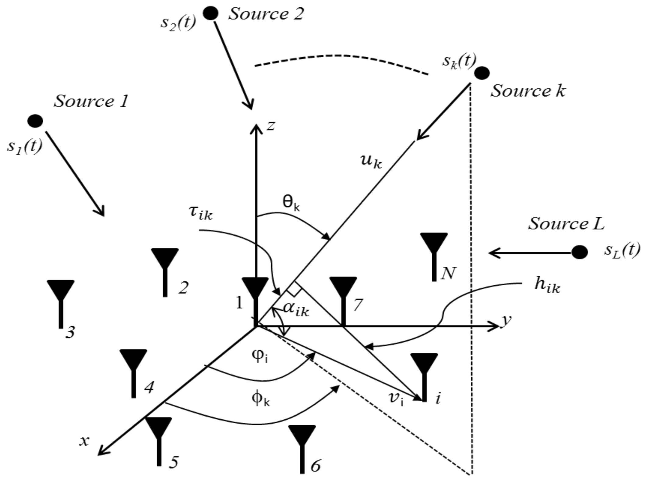
2. AoA Model and Problem Formulation

It is assumed that L narrowband signals, arriving from different elevation (${\theta }_j$) and azimuth angles (${\varphi }_j$) angles are incident on an arbitrary antenna array, as shown in Figure 1 [36]. The signal sources are assumed to lie in the far-field. At the receiving end, these signals are received by M sensors and processed digitally to determine their DoAs.

The total received baseband signal, $\mathit{X}\left(t\right)$ under Gaussian noise channel conditions is given as follows:

$$\mathit{X}\left(t\right)=\mathit{A}\left(\theta , \varphi \right) \mathit{S}\left(t\right)+\mathit{N}\left(t\right)$$

(1)

where:

• $\mathit{S}\left(t\right)={\left[{\mathit{s}}_{\mathbf{1}}\left(t\right),{\mathit{s}}_{\mathbf{2}}\left(t\right),\dots , {\mathit{s}}_{\mathit{L}}\left(t\right)\right]}^{\mathit{T}}$ is a Binary Phase Shift Keying (BPSK) modulated signal.
• $\mathit{N}\left(t\right)=\left[{\mathit{n}}_{\mathbf{1}}\left(t\right), {\mathit{n}}_{\mathbf{2}}\left(t\right), \dots , {\mathit{n}}_{\mathit{M}}\left(t\right)\right]$ is an AWGN for each channel.
• $\mathit{A}\left(\theta , \varphi \right)$ is the M × L matrix of steering vectors and is defined as follows:

  $$\mathit{A}(\theta , \varphi )=\left[\mathit{a}({\theta }_1, {\varphi }_1) \mathit{a}({\theta }_2, {\varphi }_2) \dots \mathit{a}({\theta }_L, {\varphi }_L)\right]$$

  (2)

With k signals impinging on the above array, the unit vector defining the incidence azimuth and elevations angles of one signal is described below:

$${\mathit{u}}_{\mathit{k}}=\cos {\varphi }_k\sin {\theta }_k{\widehat{a}}_x+\sin {\varphi }_k\sin {\theta }_k{\widehat{a}}_y+\cos {\theta }_k{\widehat{a}}_z$$

(3)

where, ${\widehat{a}}_x, {\widehat{a}}_y,$ and ${\widehat{a}}_z$ are the unit vectors for Cartesian co-ordinates. The unit vector that measures the distance from an original reference point to the i’th element can be given below:

$${\mathit{v}}_{\mathit{i}}=r_i\cos {\phi }_i{\widehat{a}}_x+r_i\sin {\phi }_i{\widehat{a}}_y, i= 1, 2, \dots , M.$$

(4)

Here, ${\phi }_i$ represents the angular separation between the x-plane and the locations of the ith element. Next, the angles (${\mathit{\alpha }}_{\mathit{i}\mathit{k}}$) should be calculated from the dot product between unit vectors ${\mathit{v}}_{\mathit{i}}$ and ${\mathit{u}}_{\mathit{k}}$, as below:

$${\alpha }_{ik}={\cos }^{-1}\left(\frac{v_i·u_k}{\left|\right|v_i\left|\right|·\left|\right|u_k\left|\right|}\right)={\cos }^{-1}\left(\frac{\sin {\theta }_k\cos ({\varphi }_k-{\phi }_i)}{\left|\right|v_i\left|\right|·\left|\right|u_k\left|\right|}\right)={\cos }^{-1}\left(\sin {\theta }_k\cos ({\varphi }_k-{\phi }_i)\right)$$

(5)

The whole set of produced angles due to L signals incident on M elements can be constructed as a matrix, as described below:

$${{\rm Y}}_{\mathit{i}\mathit{k}}= \left[\begin{array}{cccc}{\alpha }_{11}& {\alpha }_{12}& \cdots & {\alpha }_{1L}\\ {\alpha }_{21}& {\alpha }_{22}& ⋮& {\alpha }_{2L}\\ ⋮& ⋮& \ddots & ⋮\\ {\alpha }_{M1}& {\alpha }_{M2}& \cdots & {\alpha }_{ML}\end{array} \right]$$

(6)

The corresponding time delay, ${\mathit{\tau }}_{\mathit{i}\mathit{k}}$, of each ${\mathit{\alpha }}_{\mathit{i}\mathit{k}}$ can be computed as follows:

$${\tau }_{ik}=r\cos {\alpha }_{ik}= r\cos \left({\cos }^{-1}\left(\sin {\theta }_k\cos ({\varphi }_k-{\phi }_i)\right)\right)=r\sin {\theta }_k\cos ({\varphi }_k-{\phi }_i)$$

(7)

The matrix that includes the time delays of all incident signals on M sensors can be given as follows:

$${\mathit{{\rm T}}}_{\mathit{i}\mathit{k}}=\left[\begin{array}{cccc}{\tau }_{11}& {\tau }_{12}& \cdots & {\tau }_{1L}\\ {\tau }_{21}& {\tau }_{22}& ⋮& {\tau }_{2L}\\ ⋮& ⋮& \ddots & ⋮\\ {\tau }_{M1}& {\tau }_{M2}& \cdots & {\tau }_{ML}\end{array}\right]$$

(8)

The angular phase difference (${\psi }_{ik}$) is presented below:

$${\psi }_{ik}=\beta {\tau }_{ik}=\frac{2\pi }{\lambda }r\sin {\theta }_k\cos ({\varphi }_k-{\phi }_i)$$

(9)

where, $\lambda$ is the wavelength. Then, the corresponding phase difference of the ${\mathit{T}}_{\mathit{i}\mathit{k}}$ can be presented as follows:

$${\mathit{\psi }}_{\mathit{i}\mathit{k}}=\left[\begin{array}{cccc}{\psi }_{11}& {\psi }_{12}& \cdots & {\psi }_{1L}\\ {\psi }_{21}& {\psi }_{22}& ⋮& {\psi }_{2L}\\ ⋮& ⋮& \ddots & ⋮\\ {\psi }_{M1}& {\psi }_{M2}& \cdots & {\psi }_{ML}\end{array}\right]$$

(10)

The array steering vector of the above antenna array under these assumptions and conditions can be defined as follows:

$$\mathit{a}({\theta }_k, {\varphi }_k)=\left[\begin{array}{ccc}{e}^{-j{\psi }_{1k}}& \begin{array}{cc}{e}^{-j{\psi }_{2k}}& \cdots \end{array}& e^{-j{\psi }_{Mk}}\end{array}\right]$$

(11)

3. The Projection Matrix Construction

It is well-known that the subspace AoA techniques are very sensitive to under- or over-estimation of the sources number L, where any mistake in this estimation can cause a poor resolution. Although the PM method is classified as a subspace method, it does not need to separate the signal and noise subspaces. In this work, it is shown that the PM method can work without the need to know the number of arriving signals. Considering that M receivers are used to measure the data of impinging signals at N times, then the received data matrix, $\mathit{X}\left(\mathit{t}\right)$, can be given as follows:

$$\mathit{X}\left(\mathit{t}\right)=\left[\begin{array}{c}\begin{array}{c}{x}_1\left(t_1\right)\\ x_2\left(t_1\right)\\ ⋮\end{array}\\ ⋮\\ x_M\left(t_1\right)\end{array} \begin{array}{c}\begin{array}{c}{x}_1\left(t_2\right)\\ x_2\left(t_2\right)\\ ⋮\end{array}\\ ⋮\\ x_M\left(t_2\right)\end{array} \begin{array}{c}\begin{array}{c}\cdots \\ ⋮\\ \ddots \end{array}\\ ⋮\\ \dots \end{array} \begin{array}{c}\begin{array}{c}\cdots \\ ⋮\\ ⋮\end{array}\\ \ddots \\ \dots \end{array} \begin{array}{c}\begin{array}{c}{x}_1\left(t_{\mathit{N}}\right)\\ x_2\left(t_{\mathit{N}}\right)\\ ⋮\end{array}\\ ⋮\\ x_M\left(t_{\mathit{N}}\right)\end{array}\right]$$

(12)

Once the received data matrix is measured, one needs to compute the array covariance matrix (${\mathit{ℛ}}_{\mathit{x}\mathit{x}}$) as follows:

$$\begin{gathered} {\mathit{ℛ}}_{\mathit{x}\mathit{x}}=\mathit{E}\left[\mathit{X}\left(t\right) {\mathit{X}}^{\mathit{H}}\left(t\right)\right]=\left[\mathit{A}\left(\theta , \varphi \right) \mathit{S}\left(t\right){\mathit{S}}^H\left(\mathit{t}\right)\mathit{A}{\left(\theta , \varphi \right)}^H\right]+\mathit{E}\left[\mathit{N}\left(t\right) {\mathit{N}}^H\left(t\right)\right] \\ {\mathit{ℛ}}_{\mathit{x}\mathit{x}}=\mathit{A}\left(\theta , \varphi \right) {\mathit{ℛ}}_{\mathit{s}\mathit{s}}\mathit{A}{\left(\theta , \varphi \right)}^H+{\sigma }_n{}^{\mathbf{2}}{\mathit{I}}_{\mathit{M}} \end{gathered}$$

(13)

where, ${\mathit{ℛ}}_{\mathit{s}\mathit{s}}$ is the (L × L) source signal correlation matrix ${\mathit{ℛ}}_{\mathit{s}\mathit{s}}=\mathit{E}\left(\mathit{S}\left(t\right)\mathit{S}\left(t\right)\right)$, ${{\sigma }_n}^2$ is the noise variance, ${\mathit{I}}_{\mathit{M}}$ is the M × M identity matrix, and $\mathit{H}$ denotes the Hermitian transpose.

When some or all of the signals’ sources are non-stationary, in other words when they move from one location to another during the estimation or tracking process time, the directions of their sent signals will change, and thus, the directions of emitted signals will arrive at the receiving array end from different angles. This means $\mathit{A}\left(\theta , \varphi \right)$ can be changed partially or completely and consequently the spatial spectrum of the ${\mathit{ℛ}}_{\mathit{x}\mathit{x}}$ will change. To this end, the covariance matrix needs to be measured frequently in the practical applications to ensure reliable estimation. A complete knowledge of ${\mathit{ℛ}}_{\mathit{x}\mathit{x}}$ cannot be assumed, instead, we may use as necessary the sample-average estimated array input auto-covariance matrix given by:

$${\widehat{\mathit{ℛ}}}_{\mathit{x}\mathit{x}}\approx \frac{1}{N}{\displaystyle \sum }_{k=1}^N\mathit{X}\left(t\right){\mathit{X}}^H\left(t\right)$$

(14)

The Capon method [12] needs to calculate the inverse of the CM and, therefore, its spatial spectrum can be defined as follows:

$${\mathit{P}}_{\mathit{C}\mathit{a}\mathit{p}\mathit{o}\mathit{n}}(\theta ,\phi )=\frac{1}{\mathit{a}(\theta ,\phi ){\mathit{ℛ}}_{\mathit{x}\mathit{x}}^{-1}\mathit{a}{(\theta ,\phi )}^{\mathit{H}}}$$

(15)

Alternatively, the idea of the propagator method [24] is to divide the covariance matrix into two sub-matrices, as described below:

$${\mathit{ℛ}}_{\mathit{x}\mathit{x}}=\left[\begin{array}{c}{\mathit{ℛ}}_{\mathbf{1}}\\ {\mathit{ℛ}}_{\mathbf{2}}\end{array}\right]\begin{array}{c}\}\\ \}\end{array}\begin{array}{c}\mathrm{L}\\ M-L\end{array}$$

(16)

By considering ${\mathit{ℛ}}_{\mathbf{1}}$ is a non-singular matrix, the propagator may be defined as a unique linear operator $\mathcal{P}$ of C^M-L into C^L. In the noiseless system, the propagator is given as follows:

$${\mathit{ℛ}}_{\mathbf{2}}={\mathcal{P}}^{\mathit{H}}{\mathit{ℛ}}_{\mathbf{1}}$$

(17)

However, when the environment is noisy, the least mean square (LMS) method is used to estimate $\mathcal{P}$ as expressed below,

$$\mathcal{P}={\left({\mathcal{R}}_{\mathbf{1}}^{\mathit{H}}{\mathit{ℛ}}_{\mathbf{1}}\right)}^{-1}{\mathcal{R}}_{\mathbf{1}}^{\mathit{H}}{\mathit{ℛ}}_{\mathbf{2}}$$

(18)

Next, we need to construct a $\mathcal{V}$ matrix, such that:

$$\mathcal{V}=[{\mathcal{P}}_{\mathit{H}}-{\mathit{I}}_{\mathit{M}-\mathit{L}}]$$

(19)

${\mathit{I}}_{\mathit{M}-\mathit{L}}$ is the identity with dimension (M - L) × M. The spatial spectrum of the propagator method can be constructed as follows:

$${\mathit{P}}_{propagator}(\theta ,\phi )=\frac{\mathbf{1}}{{\left|\right|\mathit{a}(\theta ,\phi )\mathit{V}\left|\right|}^2}$$

(20)

For the subspace methods, one needs to apply the Eigenvalue Decomposition (EVD) approach to ${\mathit{ℛ}}_{\mathit{x}\mathit{x}}$ and then sorting the eigenvalues in a descending way yields:

$${\mathit{ℛ}}_{\mathit{x}\mathit{x}}=\mathit{Q} \mathit{\Sigma }{\mathit{Q}}^H=\left[{\mathit{Q}}_{\mathit{S}\mathit{S}} {\mathit{Q}}_{\mathit{N}\mathit{S}}\right] \left[\begin{array}{cc}{\Sigma }_{\mathit{S}\mathit{S}}& 0\\ 0& {\Sigma }_{\mathit{N}\mathit{S}}\end{array}\right]\left[\begin{array}{c}{\mathit{Q}}_{\mathit{S}\mathit{S}}^H\\ {\mathit{Q}}_{\mathit{N}\mathit{S}}^H\end{array}\right]$$

(21)

${\mathit{Q}}_{\mathit{S}\mathit{S}}=\left({\mathit{q}}_{\mathit{1}}, {\mathit{q}}_{\mathit{2}}, \dots \dots , {\mathit{q}}_{\mathit{L}}\right)$ is the Signal Subspace (SS) matrix, which associates with L largest eigenvalues, ${\mathit{\Sigma }}_{\mathit{S}\mathit{S}}=\left({\Sigma }_1,{\Sigma }_2,\dots \dots ,{\Sigma }_L\right)$. whereas ${\mathit{Q}}_{\mathit{N}\mathit{S}}=\left({\mathit{q}}_{\mathit{L}+\mathit{1}}, {\mathit{q}}_{\mathit{L}+\mathit{2}}, \dots \dots , {\mathit{q}}_{\mathit{M}}\right)$ represents a Noise Subspace (NS) matrix, which is associated with the M-L lowest eigenvalues, ${\mathit{\Sigma }}_{\mathit{N}\mathit{S}}=\left({\Sigma }_{L+1},{\Sigma }_{L+2},\dots \dots ,{\Sigma }_M\right).$ MUSIC exploits the orthogonality between the manifold vector (i.e., steering vector) and the eigenvectors of the NS to determine the directions of arrival signals. The spatial spectrum of the MUSIC method can be constructed as follows [19]:

$${\mathit{P}}_{\mathit{M}\mathit{U}\mathit{S}\mathit{I}\mathit{C}}\left(\theta ,\varphi \right)=\frac{1}{\mathit{a}(\theta ,{ }_{ }\varphi ){\mathit{Q}}_{\mathit{N}\mathit{S}} {\mathit{Q}}_{\mathit{N}\mathit{S}}{}^{\mathit{H}}\mathit{a}{(\theta , \varphi )}^{\mathit{H}}}$$

(22)

Alternatively, one can exploit the orthogonality between the manifold vector and SS to estimate the AoAs. To achieve this task, projections of the L eigenvectors (i.e., ${\mathit{Q}}_{\mathit{S}\mathit{S}}$) should be calculated first as follows [39]:

$${\mathcal{U}}_{\mathit{S}\mathit{S}}={\mathit{I}}_{\mathit{M}}-{\mathit{Q}}_{\mathit{S}\mathit{S}}{\left({\mathit{Q}}_{\mathit{S}\mathit{S}}{}^H {\mathit{Q}}_{\mathit{S}\mathit{S} }\right)}^{-1 }{\mathit{Q}}_{\mathit{S}\mathit{S}}{}^H$$

(23)

Then, the pseudo-spectrum of the PM method based on the SS matrix can be constructed as follows [37]:

$${\mathit{P}}_{PM/{\mathcal{U}}_{SS}}\left(\theta ,\varphi \right)=\frac{1}{\mathit{a}(\theta ,{ }_{ }\varphi ){\mathcal{U}}_{\mathit{S}\mathit{S}} {\mathcal{U}}_{\mathit{S}\mathit{S}}{}^{\mathit{H}}\mathit{a}{(\theta , \varphi )}^{\mathit{H}}}$$

(24)

With this assumption, the construction of the projection matrix is based on the SS eigenvectors, and therefore, the decomposition of the CM is required. Instead, it can directly exploit L rows/columns of the CM to construct a projection matrix without the need to decompose the CM. Consider the observed CM defined as follows:

$${\mathit{ℛ}}_{\mathit{x}\mathit{x}}=\mathit{X}\left(\mathit{t}\right) \mathit{X}{\left(\mathit{t}\right)}^H=\left[\begin{array}{c}\begin{array}{c}{r}_{11}\\ r_{21}\end{array}\\ ⋮\\ r_{M1}\end{array} \begin{array}{c}\begin{array}{c}{r}_{12}\\ r_{22}\end{array}\\ ⋮\\ r_{M2}\end{array} \begin{array}{c}\begin{array}{c}\cdots \\ ⋮\end{array}\\ \ddots \\ \dots \end{array} \begin{array}{c}\begin{array}{c}{r}_{1L}\\ r_{2L}\end{array}\\ ⋮\\ r_{ML}\end{array} \begin{array}{cc}\begin{array}{c}\cdots \\ ⋮\end{array}& \begin{array}{c}{r}_{1M}\\ r_{2M}\end{array}\\ \ddots & ⋮\\ \dots & r_{MM}\end{array}\right]$$

(25)

In this case, one needs to select L rows/columns of ${\mathit{ℛ}}_{\mathit{x}\mathit{x} }$ to sample ${\mathit{Q}}_{\mathit{L}}$ as given below:

$${\mathit{Q}}_{\mathit{L}}=\left[\begin{array}{c}\begin{array}{c}{r}_{11}\\ r_{21}\end{array}\\ ⋮\\ r_{M1}\end{array} \begin{array}{c}\begin{array}{c}{r}_{12}\\ r_{22}\end{array}\\ ⋮\\ r_{M2}\end{array} \begin{array}{c}\begin{array}{c}\cdots \\ ⋮\end{array}\\ \ddots \\ \dots \end{array} \begin{array}{c}\begin{array}{c}{r}_{1L}\\ r_{2L}\end{array}\\ ⋮\\ r_{ML}\end{array} \right]$$

(26)

Then, the projection matrix based on ${\mathit{Q}}_{\mathit{L}}$ can be computed as follows:

$${\mathcal{U}}_{\mathit{L}}={\mathit{I}}_{\mathit{M}}-{\mathit{Q}}_{\mathit{L}}{\left({\mathit{Q}}_{\mathit{L}}{}^{\mathit{H}} {\mathit{Q}}_{\mathit{L}}\right)}^{-\mathit{1}}{\mathit{Q}}_{\mathit{L}}{}^H$$

(27)

The pseudo-spectrum of the PM method using ${\mathcal{U}}_{\mathit{L}}$ can be constructed using the following formula.

$${\mathit{P}}_{PM/{\mathcal{U}}_L}\left(\theta ,\varphi \right)=\frac{1}{\mathit{a}(\theta , \varphi ){\mathcal{U}}_{\mathit{L}} {\mathcal{U}}_{\mathit{L}}{}^H\mathit{a}{(\theta , \varphi )}^H}$$

(28)

The working principle of the above formula still depends on the previous knowledge of the number of arrival signals, which is difficult in the practical applications. Thus, a pre-processing is required to find the actual number of arrival signals, and this, in turn, will increase the computational complexity. Therefore, in the next section, the projection matrix will be formed regardless of the number of arrival signals.

4. The Methodology of Matrix Sampling

The way of sampling the rows/columns of a matrix has a substantial influence on estimating the eigenvalues and eigenvectors of the covariance matrix [40,41]. Volume sampling is the picking of k-subsets of the rows/columns of a certain matrix with probabilities proportional to the squared volumes of the simples defined by them. It was first introduced in Reference [42] in the context of low-rank approximation of matrices. The problem at hand is to find a method that can increase the estimation resolution of the PM method without increasing M. Thus, our approach is based on picking a P-subset of rows of M ∈ C^M×P so that projecting onto their span can provide sufficient information about the incident signals but without raising the computational burden of a complete spectral analysis significantly. This problem is identical to the column-subset problem of the matrix transpose mentioned in Reference [40].

The PM method assumes the number of arrival signals is known and less than a number of array sensors [43]. However, it is considered a low-complexity method since it does not need to compute the inversion or decomposition of the CM, as is done in the Capon and MUSIC methods, respectively. Although the PM method that is defined in Equation (28) is categorized as a signal subspace method, where L should be known in advance, it seems this assumption is not entirely accurate since the SS and NS matrices are obtained after applying EVD. Therefore, there is no need to separate these matrixes in order to calculate the projection matrix.

Hence, a new projection matrix will be constructed based on selecting P rows/columns instead of using only L, where L ≤ P < M. Under this assumption, the PM method will be considered as a blind method. Then, the estimation accuracy of the PM method will depend mainly upon the value of P; ${\mathit{Q}}_{\mathit{P}}$ can be defined as described below;

$${\mathit{Q}}_{\mathit{P}}=\left[\begin{array}{c}\begin{array}{c}{r}_{11}\\ r_{21}\end{array}\\ ⋮\\ r_{M1}\end{array} \begin{array}{c}\begin{array}{c}{r}_{12}\\ r_{22}\end{array}\\ ⋮\\ r_{M2}\end{array} \begin{array}{c}\begin{array}{c}\cdots \\ ⋮\end{array}\\ \ddots \\ \dots \end{array} \begin{array}{c}\begin{array}{c}{r}_{1P}\\ r_{2P}\end{array}\\ ⋮\\ r_{MP}\end{array} \right]$$

(29)

The way and selected sampling size of (29) can affect significantly on the signal parameters estimations. To justify this point, one can investigate the relationship between the sampled matrices and the obtained eigen/singular values of the L arrival signals. It is known the estimation accuracy is directly proportional to the power of the eigenvalues. To this end, a covariance matrix that contains data for seven signals is generated randomly with size (30 × 30). Then, ${\mathit{Q}}_{\mathit{P}}$ has been sampled based on different values of P namely: P = ( 7, 10, 15, 20, 24, 27), where the Singular Value Decomposition (SVD) applied to each sampled matrix as follows:

$${\mathit{Q}}_{\mathit{P}}=\mathit{U} \Sigma {\mathit{V}}^{\mathit{H}}$$

(30)

The summation of the L largest singular values for each sampled matrix is calculated as follows:

$$SV={\displaystyle \sum }_{i=1}^L{\mathsf{\Sigma }}_i$$

(31)

The calculated results are plotted as a Cumulative Distribution Function (CDF), as shown in Figure 2. Apparently, the obtained power of the L dominated singular values increased significantly with the increasing number of sampled columns. Thus, one can improve the performance of the PM method by increasing only the number of sampled columns at the projection matrix construction step. Then, the projection matrix based on the proposed sampled matrix, ${\mathit{Q}}_{\mathit{P}}$, can be computed as follows:

$${\mathcal{U}}_{\mathit{P}}={\mathit{I}}_{\mathit{M}}-{\mathit{Q}}_{\mathit{P}} {\left({\mathit{Q}}_{\mathit{P}}{}^H {\mathit{Q}}_{\mathit{P}}\right)}^{-1} {\mathit{Q}}_{\mathit{P}}{}^H$$

(32)

Finally, the spatial spectrum of the proposed method can be constructed as given below:

$${\mathit{P}}_{prop}\left(\theta ,\varphi \right)=\frac{1}{\mathit{a}\left(\theta ,\varphi \right){\mathcal{U}}_{\mathit{P}} {\mathcal{U}}_{\mathit{P}}{}^H\mathit{a}{\left(\theta ,\varphi \right)}^H}$$

(33)

The procedures of the proposed sampling methodology for AoA estimation are given in

Table 1. Showing the simulation steps of the proposed sampling method.

Input:	The measured data matrix, $X\in C^{M\times N}$, with M receivers, N number of measurements, L incident signals.
Output:	The estimated AoAs.
Step 1:	Calculate the CM using (25)
Step 2:	Sample ${\mathit{Q}}_{\mathit{P}}$ matrix based on a specific P as follows: ${\mathit{Q}}_{\mathit{P}}={\mathcal{R}}_{\mathit{x}\mathit{x}}(:,1:\mathrm{P})$
Step 3:	Construct the projection matrix (i.e., ${\mathcal{U}}_{\mathit{P}}$) using (32)
Step 4:	Construct the pseudo spectrum using (33)
Step 5:	Find the locations of the produced peaks to determine the AoAs

.

4.1. Estimation Accuracy Analysis

In this section, it will be proven that an increase in the number of sampled columns leads to an increase in the Degrees of Freedom (DOFs). For the AoA estimation, the aim is to determine the number of the resultant nulls of the array factor instead of the number of maxima. To justify the advantage of angle resolution using the proposed sampled approach compared to the classically used one, we will compute the possible nulls produced using both methods. Using the classical sampling approach, the Array Factor (AF) based on the L selected columns can be shaped as follows:

$$\mathit{A}{\mathit{F}}_{\mathit{L}}\left(\theta \right)=\left[1 e^{-j\psi } e^{-j2\psi } \dots e^{-j\left(L-1\right)\psi }\right]$$

(34)

where $\psi = \pi \cos \theta$; multiplying both sides of the above equation by function $e^{-j\psi }$, leads to:

$$\mathit{A}{\mathit{F}}_{\mathit{L}}\left(\theta \right) e^{-j\psi }=\left[ e^{-j\psi } e^{-2j\psi } e^{-j3\psi } \dots e^{-jL\psi }\right]$$

(35)

Subtracting equation (35) from (34) results in:

$$\mathit{A}{\mathit{F}}_{\mathit{L}}\left(\theta \right)=\frac{\left(e^{-jL\psi }-1 \right) }{\left(e^{-j\psi }-1\right)}$$

(36)

which simplifies to a $\raisebox{1ex}{$\sin x$}\!\left/ \!\raisebox{-1ex}{$x$}\right.$ function:

$$\mathit{A}{\mathit{F}}_{\mathit{L}}\left(\theta \right)=\frac{\sin (L\frac{\psi }{2})}{\sin (\frac{\psi }{2})}$$

(37)

From the above equation, it can be concluded there are L-1 nulls available to point in the directions of the incident signals. For the proposed weighting methodology, it is decided to select P columns and, therefore, the array factor can be given by:

$$\mathit{A}{\mathit{F}}_{\mathit{P}}\left(\theta \right)=[1 e^{-j\psi } \dots \dots e^{-j(P-1)\psi }]$$

(38)

Multiplying both sides of the above equation by function $e^{-j\psi }$ yields:

$$\mathit{A}{\mathit{F}}_{\mathit{P}}\left(\theta \right)e^{-j\psi }=\left[e^{-j\psi } e^{-2j\psi } \dots \dots e^{-jP\psi }\right]$$

(39)

Subtracting equation (39) from (38) results in:

$$\mathit{A}{\mathit{F}}_{\mathit{P}}\left(\theta \right)=\frac{(e^{-jP\psi }-1)}{(e^{-j\psi }-1)}=\frac{\sin \left(P\frac{\psi }{2}\right)}{\sin \left(\frac{\psi }{2}\right)}$$

(40)

The generated array nulls using the proposed sampling method occur when the numerator argument $\frac{\left(P-1\right)}{2}\cos {\theta }_P=\pm n\pi$. Hence,

$${\theta }_P={\cos }^{-1}\left(\pm \frac{2n\pi }{\left(P-1\right)}\right), n=1, 2, \dots , (P-1)$$

(41)

Obviously, the total number of nulls that can be obtained from the above equation is P-1, and this number can be increased by increasing the P sampled columns. To compare the expected number of nulls that can be pointed towards the angles of the received signals between the classical and proposed sampling methodology, Equation (40) is divided by Equation (37) as follows:

$$NR=\frac{\mathit{A}{\mathit{F}}_{\mathit{P}}\left(\theta \right)}{\mathit{A}{\mathit{F}}_{\mathit{L}}\left(\theta \right)}=\frac{P-1}{L-1}$$

(42)

Based on the above arguments, the Nulls Ratio (NR) number can be increased by increasing the number of the sampled columns, which, in turn, will increase DOFs. The NR can play a significant role in adjusting the AoAs resolution to resolve very closely spaced incidents signals on the array.

4.2. The Computational Complexity Analysis

Several works in the DoA estimation area show that the linear methods such as the PM algorithm have much lower computational complexity than subspace methods [39,44]. This is because it does not require inversion or decomposition of the CM, which costs approximately O (M³), where M is a number of the antenna elements. With massive MIMO, the O (M³) entails forbiddingly high-computational complexity. Generally, obtaining limited hardware cost with large array apertures cause serious challenges for real-time signal processing and parameter estimation.

The computational burden of the projection matrix construction needs O (M²P) arithmetic operations. The PM method based on the new methodology replaces the computation of the matrix inverse with a new problem of size (M × M) by (P × P) matrix, where P is the number of selected sampled columns. Then, the calculations reduction factor of this method compared to the methods that need covariance matrix decomposition such as MUSIC, ESPRIT, etc., or the methods that require the covariance matrix inversion such as Capon is O (P/M).

Finally, the complexity of computations of the PM method at the searching grid step is O (M²${\mathrm{J}}_{\mathsf{\theta }}$), where ${\mathrm{J}}_{\mathsf{\theta }}=180/{\mathsf{\delta }}_{\mathsf{\theta }}$ and ${\mathsf{\delta }}_{\mathsf{\theta }}$ is the scanning step. As can be seen from the above Equations (24), (28), and (33), the dimensions of ${\mathcal{U}}_{\mathit{S}\mathit{S}}$, ${\mathcal{U}}_{\mathit{L}}$ and ${\mathcal{U}}_{\mathit{P}}$ are equal, which means we have the same computational burden at the grid scanning stage. The overall computational complexity of the proposed method is compared with some well-known AoA algorithms, as in

Table 2. Computational complexity comparison for several AoA methods.

Algorithm	The Needed Computational Operations
Capon	O (M3 + M2${\mathrm{J}}_{\mathsf{\theta }}$)
MUSIC	O (M3 + M2${\mathrm{J}}_{\mathsf{\theta }}$)
Propagator	O (M2 L + M2${\mathrm{J}}_{\mathsf{\theta }}$)
Original PM	O (M2 L + M2${\mathrm{J}}_{\mathsf{\theta }}$)
Proposed	O (M2 P + M2${\mathrm{J}}_{\mathsf{\theta }}$)

.

5. Numerical Simulations and Discussions

To verify the theoretical claims of this investigation, MATLAB software has been used to simulate the presented method and compare it with other AoA methods. The simulation is divided into three main scenarios: the first scenario investigates the effect of changing a number of rows/columns used (P) with SNR variations. The second scenario shows the impact of changing P with the available numbers of snapshots that are used to collect the matrix data. Finally, the proposed methodology is compared with several AoA methods in terms of the estimation accuracy and the required computational burden. Each scenario has been implemented with intensive Monte Carlo simulation to ensure a fair and robust comparison of results. In each scenario, the Average Root Mean Square Error (ARMSE) is calculated as follows:

$$\mathrm{ARMSE}=\frac{1}{K}{{\displaystyle \sum }}_{i=1}^K\sqrt{\frac{1}{L}{{\displaystyle \sum }}_{k=1}^L\left[{\left({\theta }_k-{\widehat{\theta }}_k\right)}^2\right]}$$

(43)

where, K is the number of Monte Carlo trials, ${\theta }_k$ is the randomly generated AoAs, and ${\widehat{\theta }}_k$ is the estimated AoAs. The Probability of Successful Detection (PSD) of AoAs was also computed according to the following formula:

$$\mathrm{PSD}\left(\mathrm{AoAs}\right)=\frac{{{\displaystyle \sum }}_{j=1}^{K}N{r}_j}{LK}$$

(44)

where, Nr is the number of successful-detected AoAs at each trial.

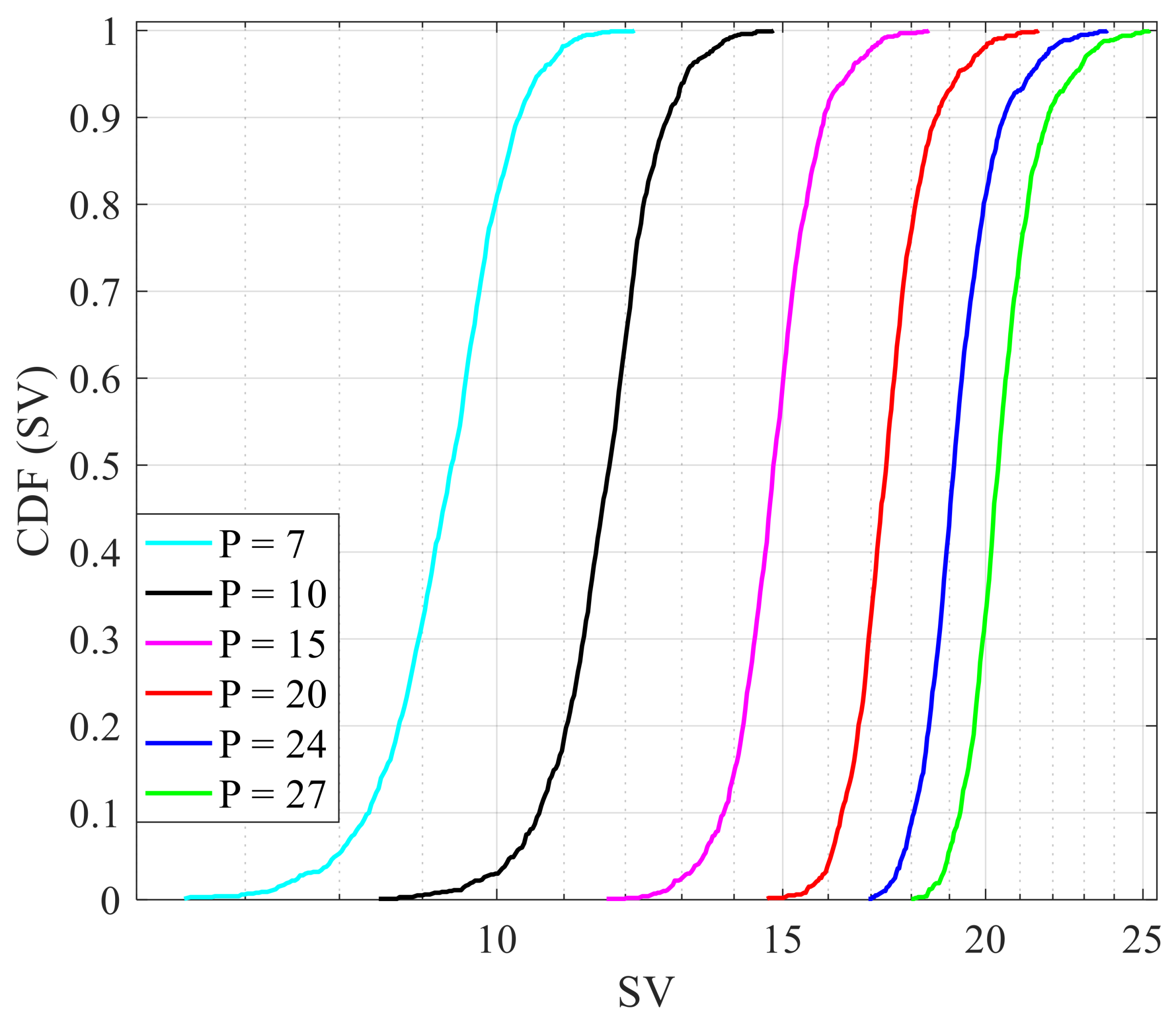
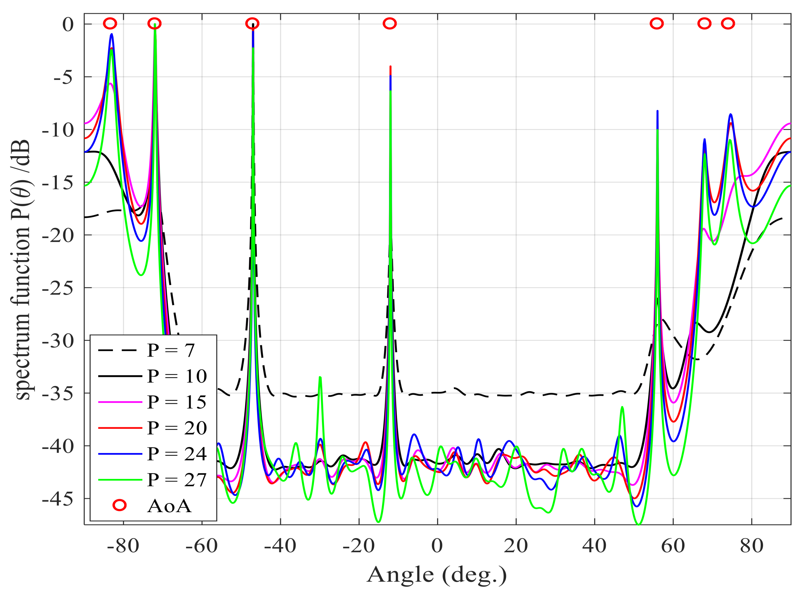
5.1. Intercomparison: Numerical Example

A numerical example is presented to show the advantage of the increasing number of sampled columns in the calculation of the projection matrix. In this example, seven plane waves (L = 7) are assumed impinging on the ULA with M = 30 and d = 0.5$\lambda$. The number of snapshots used to collect the data matrix is N =100 and the SNR at the array output is 10 dB. The scanning step angle is ${\mathsf{\delta }}_{\mathsf{\theta }}=$ 0.5°. The directions of the plane waves have been generated randomly and indicated by a red circle. Two sets of angles are supposed incident on the antenna array with close directions: the first set consists of two angles and the second of three angles. Six different values of P = (7, 10, 15, 20, 24, 27) columns have been used to construct the projection matrix.

The performance estimation of the PM method with P = L = 7 failed to detect three angles, as shown in Figure 3, whereas, its performance with P = 10 failed to detect two targets. However, with P = 15, the PM method found difficulty in resolving one of the sets with two close AoAs on the right side. At P = 20, 24, and 27, the PM method detects all the arrival angles successfully and the produced peaks become sharp and accurate. This demonstrates that the estimation resolution of the PM technique increases with increasing the number of sampled columns in the matrix projection construction stage.

However, as P increases, the computational burden is slightly increased, as shown in

Table 3. The computational burden of the PM method with a different number of sampled columns.

No. of Sampled Columns	The Computational Load
P = 7	O (3.3 × 105)
P = 10	O (3.33 × 105)
P = 15	O (3.37 × 105)
P = 20	O (3.42 × 105)
P = 24	O (3.45 × 105)
P = 27	O (3.48 × 105)

. It can be concluded the PM method is still working even with the overestimating case (i.e., P > L) and its estimation accuracy increases with increasing P.

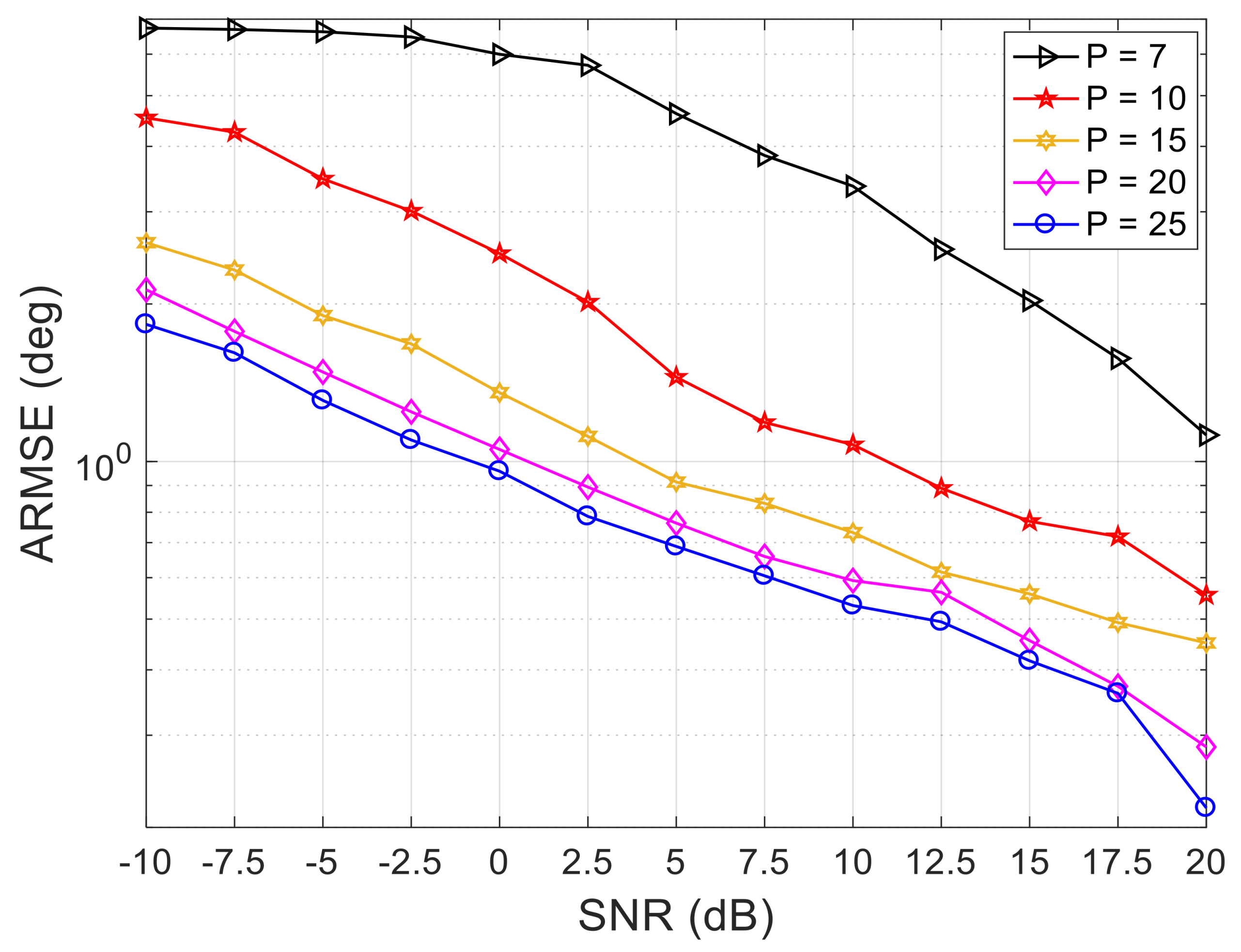
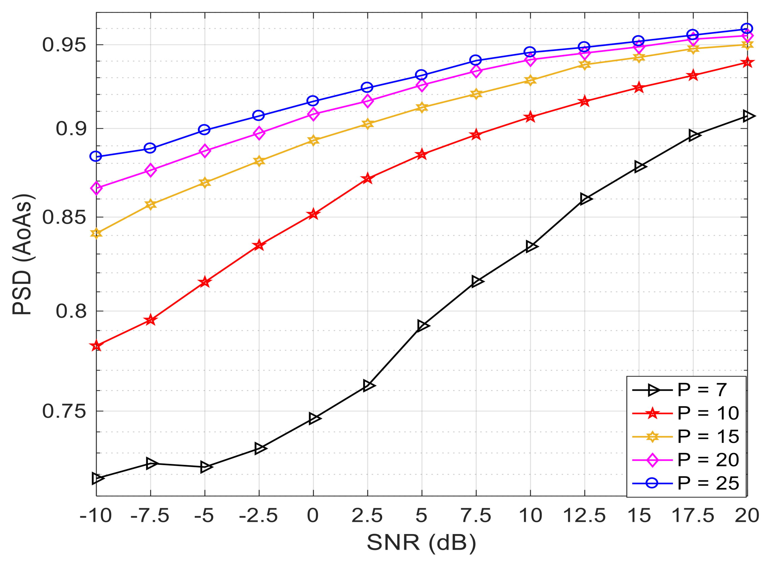
5.2. The Performance Comparison Based on the Various Signal-to-Noise Ratios (SNRs)

The SNR observed at the input to the antenna array receiver plays a crucial role in the performance estimation of direction-finding systems. This scenario investigates the variations in the performance estimation of PM methods with a variation of SNR. Five different values of P = (7, 10, 15, 20, 25) are considered in this scenario, and for each P, the SNR is assumed to vary from –10 dB to 20 dB in 2.5 dB increments. In order to investigate the effect of P values intensively, two thousand independent trials of Monte Carlo simulation (K = 2000) are carried out at each step. The 2000 sets of seven AoAs are randomly generated within the angular range (–90°, 90°), each set being applied to each P to ensure a fair comparison. The other simulation parameters are assumed the same as those given in Section 5.1. The ARMSE of every SNR is calculated and then plotted for every selected P as shown in Figure 4, whereas Figure 5 illustrates the PSD (AoAs) of the PM method at each P. Unquestionably, the ARMSE and PSD (AoAs) of the PM method are improved considerably with increased P. This is due to increasing P resulting in an increase in the aperture size of the sampled matrix and the obtained data from the covariance matrix. These advantages will enable the PM method of resolving two or many closely spaced signals with a limited number of antenna array elements.

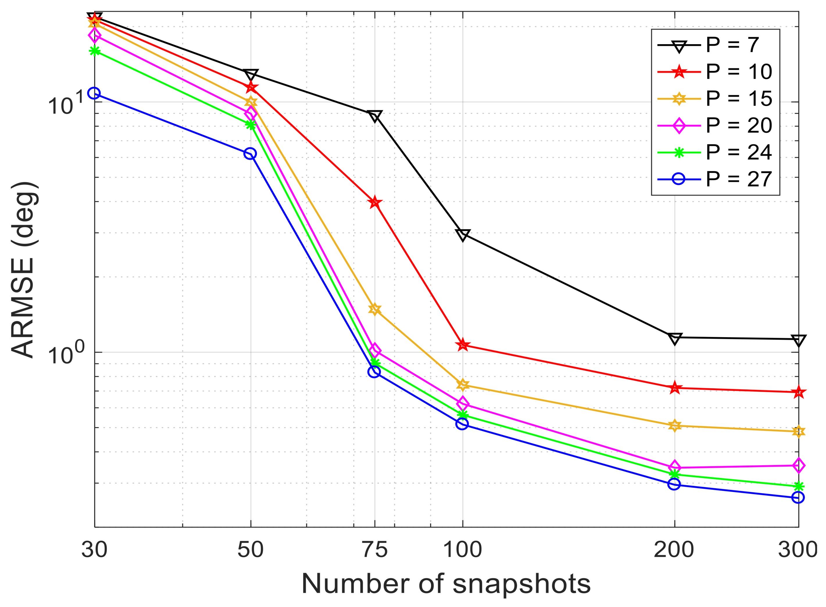
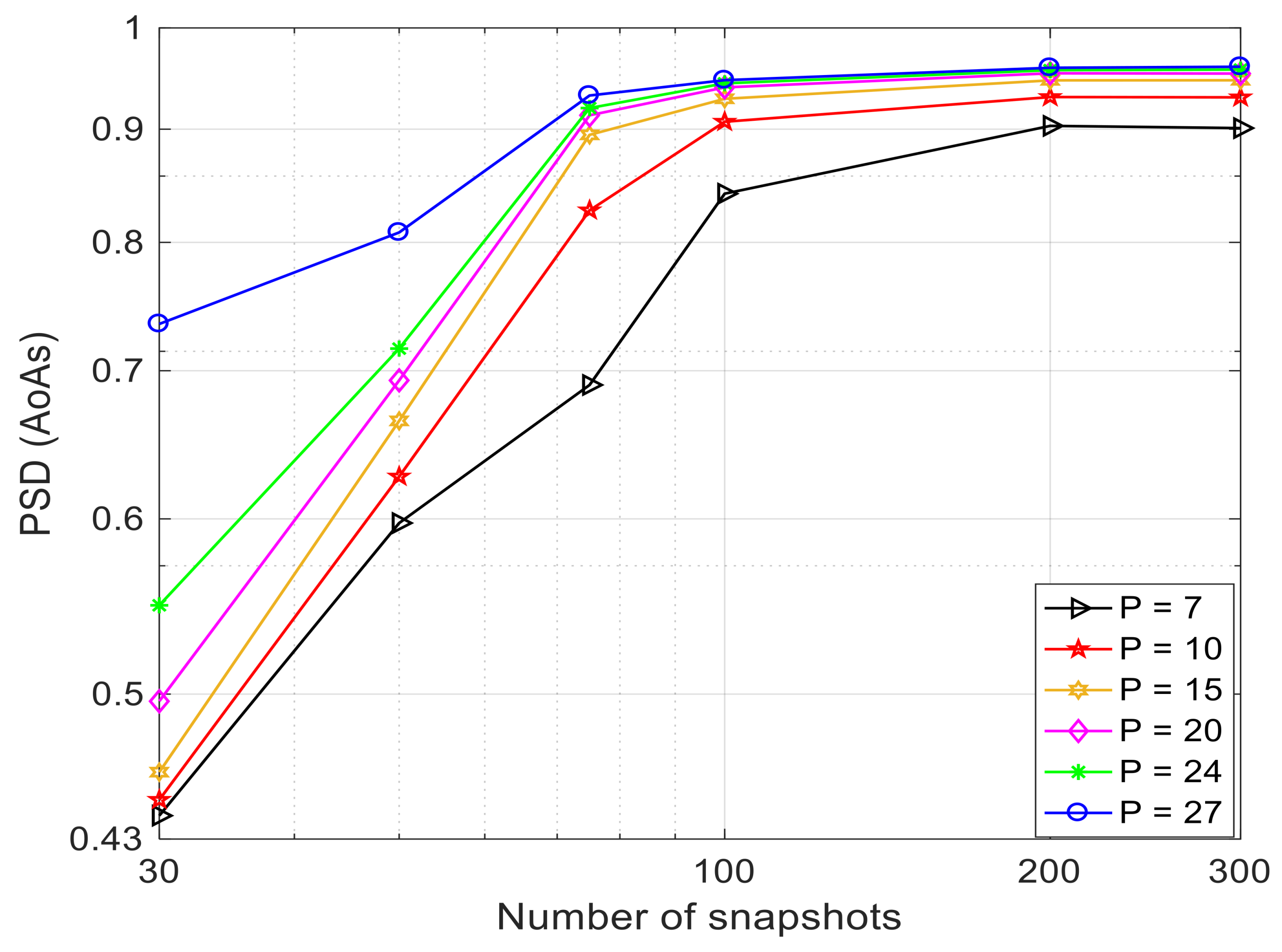
5.3. Performance Comparison Based on Different Numbers of Snapshots

The second scenario is an investigation of the number of measurements of data taken with various values of P for obtaining a reliable estimation for signals emitters. Six numbers of sampled columns have been used to construct the projection matrix, namely: P =(7, 10, 15, 20, 24, and 27). At each number of selected columns, six numbers of snapshots, namely: N = (30, 50, 75, 100, 200, and 300) with SNR = 3 dB were used to study the impact of sampled columns on the effectiveness of the projection matrix method. The other simulation parameters were the same as in the previous section, while the Monte Carlo simulation applied in Section 5.2 was considered here to ensure a reliable investigation. The ARMSE and the percentage detection probability of AoAs were computed for all the P values and are plotted in Figure 6 and Figure 7.

Clearly, increasing P increases both the estimation accuracy and the detection probability of the PM method through the whole number of snapshots range. It can be seen that any increase in the number of covariance-sampled columns improves the capability of the PM method to distinguish two or many closely spaced signals with a limited number of antenna elements. This issue has a positive effect on the localization system’s ability to detect the correct number of arrival signals without increasing the aperture size of the array. On the other hand, the computational burden of the projection matrix (${\mathcal{U}}_{\mathit{P}}$) will rise slightly.

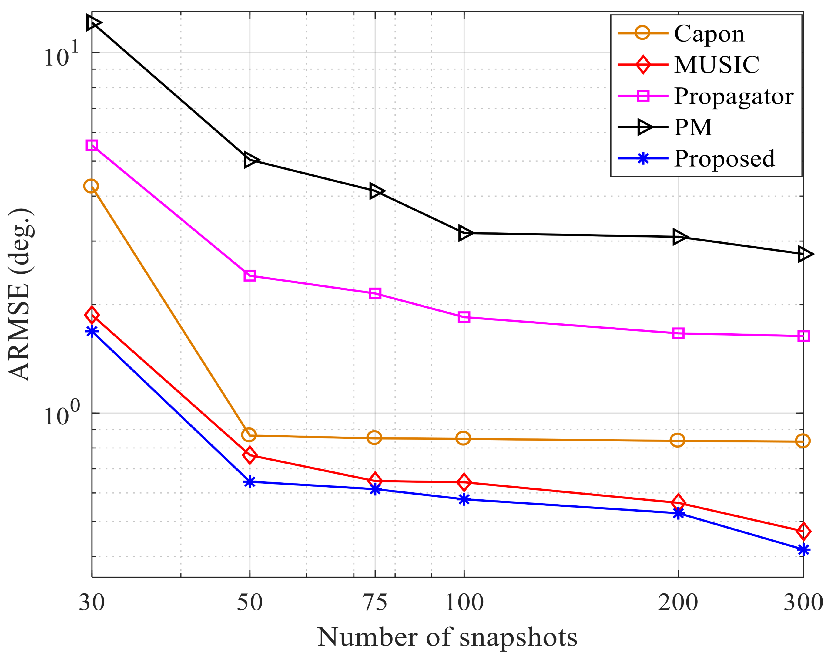
5.4. Comparison with Other AoA Methods

This section compares the performance of the PM method based on the proposed sampled matrix approach with the well-known AoA methods such as Capon, MUSIC, Propagator, and the original PM method. This comparison includes the impact of the collected number of snapshots on the estimation precision. Six values of the number of data observations are assumed namely: N = (30, 50, 75, 100, 200, 300). The number of the receivers is selected as M = 30, and the distance between the adjacent sensors is chosen as a half-wavelength. The SNR at the array output is set to 10 dB, and the proposed projection matrix is constructed based on P = 20 column samples. Two thousand Monte Carlo simulations were applied to generate the arrival angles randomly, and these were applied to all the relevant methods to ensure a fair comparison. The estimation resolution is evaluated in terms of the RMSE and. Figure 8 shows the ARMSE of each method against the number of snapshots that are used to measure the received data matrix, while Figure 9 shows the number of successfully detected angles. These graphs show that the proposed method outperforms the other methods through the whole tested range.

Notably, the proposed method can be applied directly to the covariance matrix without needing to know the number of arriving signals, unlike the MUSIC, Propagator, and the original PM methods. As can be seen from

Table 4. Required number of multiplications for each method.

Algorithm	Number of Multiplications
Capon	O (3.5 × 105)
MUSIC	O (3.5 × 105)
Propagator	O (3.3 × 105)
Original PM	O (3.3 × 105)
Proposed	O (3.4 × 105)

, the computational burden of the proposed method is less than for the Capon and MUSIC algorithms and higher than for the Propagator and original PM algorithms. However, the estimation accuracy of the presented method is significantly better than the Propagator, and original PM techniques through the whole tested range.

6. Conclusions

The effect of the matrix sampling on the covariance matrix has been investigated in this work. It was proven that the way of sampling the rows/columns of a matrix has a substantial influence on the performance of the PM algorithm. Various sampled matrices have been applied to construct the projection matrix in order to estimate the DoAs of the signals. With the proposed methodology, the PM method will not need prior knowledge of the number of arriving signals. Moreover, the estimation accuracy and PSD (AoAs) of the PM method were improved significantly without the requirement to increase the physical size of the aperture array. These improvements have been tested over a wide range of SNRs and numbers of collected data. The present method has outperformed the well-known methods and showed less computational burden compared to the MUSIC and Capon methods. The results obtained in the simulation also justified our theoretical claims.

References

1. Wan, L.; Han, G.; Shu, L.; Chan, S.; Zhu, T. The Application of DOA Estimation Approach in Patient Tracking Systems with High Patient Density. IEEE Trans. Ind. Inf. 2016, 12, 353–2364. [Google Scholar] [CrossRef]
2. Cremer, M.; Dettmar, U.; Hudasch, C.; Kronberger, R.; Lerche, R.; Pervez, A. Localization of Passive UHF RFID Tags Using the AoAct Transmitter Beamforming Technique. IEEE Sens. J. 2016, 16, 1762–1771. [Google Scholar] [CrossRef]
3. Hameed, K.W.; Al-Sadoon, M.; Jones, S.M.R.; Noras, J.M.; Dama, Y.A.S.; Masri, A.; Abd-Alhameed, R.A. Low complexity single snapshot DoA method. In Proceedings of the 2017 Internet Technologies and Applications (ITA), Wrexham, UK, 12–15 September 2017; pp. 244–248. [Google Scholar]
4. Zhang, X.; Xu, D. Angle estimation in MIMO radar using reduced-dimension capon. Electron. Lett. 2010, 46, 860–861. [Google Scholar] [CrossRef]
5. Kabir, A.L.; Saha, R.; Khan, M.A.; Sohul, M.M. Locating Mobile Station Using Joint TOA/AOA. In Proceedings of the 4th International Conference on Ubiquitous Information Technologies & Applications, Fukuoka, Japan, 20–22 December 2009; pp. 1–6. [Google Scholar]
6. Raghavan, V.; Cezanne, J.; Subramanian, S.; Sampath, A.; Koymen, O. Beamforming Tradeoffs for Initial UE Discovery in Millimeter-Wave MIMO Systems. IEEE J. Sel. Top. Signal Process. 2016, 10, 543–559. [Google Scholar] [CrossRef]
7. Zeng, Y.; Zhang, R. Millimeter Wave MIMO With Lens Antenna Array: A New Path Division Multiplexing Paradigm. IEEE Trans. Commun. 2016, 64, 1557–1571. [Google Scholar] [CrossRef]
8. Al-Sadoon, M.A.G.; Abdullah, A.S.; Ali, R.S.; Tu, Y.; Abd-Alhameed, R.A.; Jones, S.M.R.; Noras, J.M. The effects of mutual coupling within antenna arrays on angle of arrival methods. In Proceedings of the 2016 Loughborough Antennas & Propagation Conference (LAPC), Loughborough, UK, 14–15 November 2016; pp. 1–5. [Google Scholar]
9. Al-Sadoon, M.; Danjuma, I.; Abdussalam, F.; Elfergani, I.; Rodriguez, J.; Abd-Alhameed, R.; Jones, S.M.R. Dual-band compact-size antenna array for angle of arrival estimation. In Proceedings of the Loughborough Antennas & Propagation Conference (LAPC 2017), Loughborough, UK, 13–14 November 2017. [Google Scholar]
10. Al-Sadoon, M.A.G.; Asif, R.; Obeidat, H.; Bin-Melha, M.S.; Obeidat, H.; Zweid, A.; Abd-Alhameed, R.A. Low Complexity Antenna Array DOA System for Localization Applications. In Proceedings of the 6th International Conference on Wireless Networks and Mobile Communications 2018 (WINCOM), Marrakesh, Morocco, 16–19 October 2018. [Google Scholar]
11. Bartlett, M. An Introduction to Stochastic Processes with Special References to Methods and Applications; Cambridge University Press: New York, NY, USA, 1961. [Google Scholar]
12. Capon, J. High-Resolution Frequency-Wavenumber Spectrum Analysis. Proc. IEEE 1969, 57, 1408–1418. [Google Scholar] [CrossRef]
13. Gross, F. Smart Antennas for Wireless Communications; McGraw-Hill Companies Inc.: New York, NY, USA, 2005. [Google Scholar]
14. Burg, J.P. The Relationship between Maximum Entropy Spectra and Maximum Likelihood Spectra. Geophysics 1972, 37, 375–376. [Google Scholar] [CrossRef]
15. Pisarenko, V.F. The Retrieval of Harmonics from a Covariance Function. Geophys. J. R. Astrono. Soc. 1973, 33, 347–366. [Google Scholar] [CrossRef]
16. Wax, M.; Tie-Jun, S.; Kailath, T. Spatio-temporal spectral analysis by eigenstructure methods. IEEE Trans. Acoust. Speech Signal Process. 1984, 32, 817–827. [Google Scholar] [CrossRef]
17. Al-Sadoon, M.A.G.; Hameed, K.W.; Zweid, A.; Jones, S.; Abd-Alhameed, R.A.; Abusitta, M. Analysis and investigation the estimation accuracy and reliability of Pisarenko Harmonic Decomposition algorithm. In Proceedings of the 2017 Internet Technologies and Applications (ITA), Wrexham, UK, 12–15 September 2017; pp. 249–253. [Google Scholar]
18. Al-Sadoon, M.; Bin-Melha, M.; Zubo, R.; Asharaa, A.; Asif, R.; Shepherd, S. Partial Noise Subspace Method for DOA Estimation Applications. In Proceedings of the 2018 IEEE 2nd International Conference for Engineering, Technology and Sciences of Al-Kitab (2ndICETS-2018), Karkuk, Iraq, 4–6 December 2018. [Google Scholar]
19. Schmidt, R. Multiple emitter location and signal parameter estimation. IEEE Trans. Antennas Propag. 1986, 34, 276–280. [Google Scholar] [CrossRef] [Green Version]
20. Reddi, S.S. Multiple Source Location-A Digital Approach. IEEE Trans. Aerosp. Electron. Syst. 1979, AES-15, 95–105. [Google Scholar] [CrossRef]
21. Barabell, A. Improving the resolution performance of eigenstructure-based direction-finding algorithms. In Proceedings of the ICASSP ’83. IEEE International Conference on Acoustics, Speech, and Signal Processing, Boston, MA, USA, 14–16 April 1983; pp. 336–339. [Google Scholar]
22. Roy, R.; Kailath, T. ESPRIT-Estimation of Signal Parameters via Rotational Invariance Techniques. IEEE Trans. ASSP 1989, 37, 984–995. [Google Scholar] [CrossRef]
23. Munier, J.; Delisle, G.Y. Spatial analysis using new properties of the cross-spectral matrix. IEEE Trans. Signal Process. 1991, 39, 746–749. [Google Scholar] [CrossRef]
24. Marcos, S.; Marsal, A.; Benidir, M. The propagator method for source bearing estimation. Signal Process. 1995, 42, 121–138. [Google Scholar] [CrossRef]
25. Fleury, B.H.; Dahlhaus, D.; Heddergott, R.; Tschudin, M. Wideband angle of arrival estimation using the SAGE algorithm. In Proceedings of the ISSSTA’95 International Symposium on Spread Spectrum Techniques and Applications, Mainz, Germany, 25 September 1996; Volume 1, pp. 79–85. [Google Scholar]
26. Fleury, B.H.; Tschudin, M.; Heddergott, R.; Dahlhaus, D.; Pedersen, K.I. Channel parameter estimation in mobile radio environments using the SAGE algorithm. IEEE J. Sel. Areas Commun. 1999, 17, 434–450. [Google Scholar] [CrossRef]
27. Yilmazer, N.; Koh, J.; Sarkar, T.K. Utilization of a unitary transform for efficient computation in the matrix pencil method to find the direction of arrival. IEEE Trans. Antennas Propag. 2006, 54, 175–181. [Google Scholar] [CrossRef]
28. Yan, F.G.; Jin, T.; Jin, M.; Shen, Y. Subspace-based direction-of-arrival estimation using centro-symmetrical arrays. Electron. Lett. 2016, 52, 1895–1896. [Google Scholar] [CrossRef]
29. Yan, F.G.; Shen, Y.; Jin, M. Fast DOA estimation based on a split subspace decomposition on the array covariance matrix. Signal Process. 2015, 115, 1–8. [Google Scholar] [CrossRef]
30. Yan, F.G.; Cao, B.; Liu, S.; Jin, M.; Shen, Y. Reduced-complexity direction of arrival estimation with centro-symmetrical arrays and Its performance analysis. Signal Process. 2018, 142, 388–397. [Google Scholar] [CrossRef]
31. Jiang, G.; Mao, X.; Liu, Y. Direction-of-arrival estimation for uniform circular arrays under small sample size. J. Syst. Eng. Electron. 2016, 27, 1142–1150. [Google Scholar] [CrossRef]
32. Zhang, D.; Zhang, Y.; Zheng, G.; Feng, C.; Tang, J. Improved DOA estimation algorithm for co-prime linear arrays using root-MUSIC algorithm. Electron. Lett. 2017, 53, 1277–1279. [Google Scholar] [CrossRef]
33. Yan, F.G.; Wang, J.; Liu, S.; Shen, Y.; Jin, M. Reduced-Complexity Direction of Arrival Estimation Using Real-Valued Computation with Arbitrary Array Configurations. Int. J. Antennas Propag. 2018, 2018, 3284619. [Google Scholar] [CrossRef]
34. Al-Sadoon, M.A.; Abdullah, A.S.; Ali, R.S.; Al-Abdullah, A.S.; Abd-Alhameed, R.A.; Jones, S.M.R.; Noras, J.M. New and Less Complex Approach to Estimate Angles of Arrival. In Proceedings of the 8th International Conference on Wireless and Satellite Services, WiSATS 2016, Cardiff, UK, 19–20 September 2016; pp. 18–27. [Google Scholar]
35. Al-Sadoon, M.; Abduljabbar, N.; Ali, N.; Asif, R.; Zweid, A.; Alhassan, H.; Noras, J.M.; Abd-Alhameed, R.A. A More Efficient AOA Method for 2D and 3D Direction Estimation with Arbitrary Antenna Array Geometry. In Proceedings of the 8th International Conference on Broadband Communications, Networks and Systems, Faro, Portugal, 19–20 September 2018; pp. 419–430. [Google Scholar]
36. Al-Sadoon, M.A.; Ali, N.T.; Dama, Y.; Zuid, A.; Jones, S.M.R.; Abd-Alhameed, R.A.; Noras, J.M. A New Low Complexity Angle of Arrival Algorithm for 1D and 2D Direction Estimation in MIMO Smart Antenna Systems. Sensors 2017, 17, 2631. [Google Scholar] [CrossRef] [PubMed]
37. Gross, F. Smart Antennas with Matlab: Principles and Applications in Wireless Communication; McGraw-Hill Professional: New York, NY, USA, 2015. [Google Scholar]
38. Si, W.; Zeng, F.; Hou, C.; Peng, Z. A sparse-based off-grid DOA estimation method for coprime arrays. Sensors 2018, 18, 3025. [Google Scholar] [CrossRef] [PubMed]
39. Krim, H.; Viberg, M. Two decades of array signal processing research: The parametric approach. IEEE Signal Process. Mag. 1996, 13, 67–94. [Google Scholar] [CrossRef]
40. Deshpande, A.; Rademacher, L. Efficient volume sampling for row/column subset selection. In Proceedings of the 2010 IEEE 51st Annual Symposium on Foundations of Computer Science, Las Vegas, NV, USA, 23–26 October 2010; pp. 329–338. [Google Scholar]
41. Mestre, X. Improved estimation of eigenvalues and eigenvectors of covariance matrices using their sample estimates. IEEE Trans. Inf. Theory 2008, 54, 5113–5129. [Google Scholar] [CrossRef]
42. Deshpande, A.; Rademacher, L.; Vempala, S.; Wang, G. Matrix approximation and projective clustering via volume sampling. In Proceedings of the Seventeenth Annual ACM-SIAM Symposium on Discrete Algorithm, Miami, Florida, 22–26 January 2006; pp. 1117–1126. [Google Scholar]
43. Yeh, C.C. Projection approach to bearing estimations. IEEE Trans. Acoust. Speech Signal Process. 1986, 34, 1347–1349. [Google Scholar]
44. Godara, L.C. Application of antenna arrays to mobile communications. II. Beam-forming and direction-of-arrival considerations. Proc. IEEE 1997, 85, 1195–1245. [Google Scholar] [CrossRef] [Green Version]
Figure 1. M-Arbitrary element array with L arriving signals [36].
Inventions 04 00043 g001
Figure 2. The performance estimation of the Projection Matrix (PM) method with various P.
Inventions 04 00043 g002
Figure 3. Performance of the PM method with various numbers of sampled columns.
Inventions 04 00043 g003
Figure 4. ARMSE versus SNR comparison with different P.
Inventions 04 00043 g004
Figure 5. The PSD (AoAs) versus SNRs comparison.
Inventions 04 00043 g005
Figure 6. ARMSE versus the number of snapshots compared for various numbers of sampled columns.
Inventions 04 00043 g006
Figure 7. The corresponding detection probability of the AoAs for Figure 6.
Inventions 04 00043 g007
Figure 8. Comparison between the proposed method and other AoA techniques.
Inventions 04 00043 g008
Figure 9. The corresponding detection probability for AoAs shown in Figure 8.
Inventions 04 00043 g009