Design and Uncertainty Analysis of an AC Loss Measuring Instrument for Superconducting Magnets

Abstract

A novel instrument was designed and numerically validated for measuring AC losses in ramped superconducting magnets. These power losses are expected to be in the 1 $\mathrm{W}$ to 100 $\mathrm{W}$ range. The instrument improves metrological performance compared to existing instruments by reaching a target power loss uncertainty in the order of $0.1$ watt. This allows accurate measurement of the power losses to improve magnet modeling. A Monte Carlo analysis is used to evaluate the measurement uncertainty. Such an analysis addresses the lack of uncertainty investigation in the literature for this kind of measurement, and the proposed approach can be applied to various magnet models. The physical design of the instrument is carried out by relying on an FPGA-based acquisition platform. Results on a representative case study reveal that the target uncertainty can be reached without any compensation or correction mechanism. Instead, when aiming to use compensation or correction of the inductive magnet voltage, the sensitivity analysis points out that offset errors and time delays must be limited. This also suggests that the magnet’s inductance estimation should be improved more than the metrological performance of the instrumentation.

1. Introduction

During the acceleration phase of a particle beam, it is necessary to precisely adjust the magnetic field generated by the magnets. This is crucial for maintaining the correct bending and focus strength needed to ensure the proper beam operation [1]. Therefore, non-continuous magnetic fields are key elements for particle accelerators [2,3,4]. Moreover, the advent of superconducting materials enabled the possibility of reaching higher fields, thus enhancing their performance. Replacing normal conducting magnets with superconducting ones would enable more compact and efficient machines [5], especially when high-temperature superconductors (HTSs) are used. However, they must be held at cryogenic temperatures during operation.

Ideally, superconducting particle accelerator magnets dissipate no energy when operated in direct-current mode [6]. Meanwhile, energy losses are generated due to the induced voltages caused by transients [7,8] and they need to be compensated by the cooling system. As an example, magnets operated in a ramped regime became of particular interest for hadron therapy [9,10,11]. In cases like this, minimizing the usage of cryogenic fluids is desirable and, therefore, estimating the alternated current (AC) losses became crucial [5,10].

When operating superconducting magnets in non-continuous regimes, power losses are induced in the superconducting coils and in metallic elements [8]. Energy is released due to the coupling between superconducting filaments within a single wire and between different wires in the coils. Additionally, variations in the magnetic field cause fluxon movement in the filaments, leading to heat dissipation due to magnetization losses [7]. Another contribution loss arises from the magnetic response of ferromagnetic materials subjected to the external variation of the field. Finally, a role is played by the eddy currents induced in the metallic elements of the magnet [8].

AC power losses are typically modeled (analytically or numerically) during the magnet design, and they are expected to increase with an increasing ramp rate mainly due to eddy currents [2,8]. The heat released during magnet transients leads to an increase in the local temperature of the superconductor. This has to be monitored to avoid a transition to the normal conducting regime, that is, to protect the magnet from quenches and a sudden release of magnetic energy in the system [12].

Existing power loss measurement methods for superconducting devices can be macroscopically divided into calorimetric approaches and electromagnetic ones [13]. The former rely on assessing the dissipated power through the volume of evaporated cryogenic fluid or from its temperature rise [14]. Going beyond traditional boil-off methods, the resolution of these methods can be as low as 1 $\mathrm{m}$$\mathrm{W}$, e.g., by measuring evaporation losses [15]. However, to reduce the uncertainty, it is necessary to correct the heat leaks due to the current leads [16], and the cryostat must be properly designed, notably in the case of superconducting magnets [17]. In addition, calorimetric methods are time consuming, the bandwidth is typically limited to the order of 100 $\mathrm{Hz}$, and the measurement accuracy is in the order of 1% to 10% [13].

The electromagnetic methods are fast, sensitive, and accurate. Among these, electrical approaches are preferred to magnetic ones because they can measure the total AC losses [13] and are less sensitive to external magnetic fields [13,18]. These rely on the acquisition of current and voltage across the superconducting device [19,20,21]. They can be implemented with data acquisition boards to collect sampled versions of electrical quantities, which can be then digitally processed [18]. Their bandwidth reaches 10 $\mathrm{k}$$\mathrm{Hz}$ to 100 $\mathrm{k}$$\mathrm{Hz}$ with a resolution below 1 $\mathsf{\mu }$$\mathrm{W}$ [13,18,22]. Because of their advantages, electrical measurements were also considered in the present work to build a versatile and accurate measuring system for AC losses in superconducting magnets.

Electrical approaches also have limitations. Some studies comment that they are inappropriate for AC loss measurement in HTS coils with high inductance [23], and that compensation mechanisms are needed [24]. Moreover, integrating the voltage–current product merely works under periodic current conditions [13,22]. Another aspect concerns the claimed measurement accuracy. Accurate measurement of AC power losses requires identifying sources of uncertainty and performing a comprehensive uncertainty evaluation, but the existing literature lacks research focused on this aspect. Indeed, numerous studies provide AC loss measurement results for a wide variety of magnets [1,7,8,25]. Other studies also compared measurement results with simulations results [22,26]. However, the role of the measurement uncertainty in influencing power loss estimation remains unclear and insufficiently addressed. In addition, the metrological performances mentioned above are typically retrieved for superconducting devices in general, while they appear to be missing in the specific case of superconducting magnets.

The lack of uncertainty analysis in the measurement process, combined with the reliance on custom-designed electronics rather than commercial instruments, has a two-fold implication: (i) it prevents an accurate validation of numerically evaluated AC loss models, and (ii) it limits the optimization of instrumental components to improve measurement performance. Since these measurements are essential for validating loss models, any uncertainty directly affects the certification of the cooling systems and it becomes especially critical for the thermal design of conduction-cooled magnets based on cryocoolers. Instead, evaluating measurement uncertainty and investigating its sources would pave the way to the higher performance needed for AC loss assessment in superconducting magnets.

Therefore, this paper proposes the physical design and inherent uncertainty analysis of a measuring system for AC losses. This will be applied to the characterization of ramped superconducting magnets within the IRIS [27]. The novelty resides in the adoption of system components that achieve the required metrological performance into a Monte Carlo analysis to investigate measurement uncertainty by design.

In the remainder of this paper, Section 2 presents the application domain for the proposed instrument while evidencing the metrological requirements; Section 3 describes the conceptual and the physical design of the instrument, as well as the simulation setup for its numerical validation; Section 4 presents the validation results in terms of the uncertainty analyses and sensitivity analysis carried out on a representative case study; and conclusions and future developments are finally addressed in Section 5.

2. Application Domains

The design and numerical validation of the AC loss measuring system were carried out within the Innovative Research Infrastructure on Applied Superconductivity (IRIS) [27,28]. IRIS has been established in Italy as a collaboration between three national institutes and five universities, and it consists of a spread network of laboratories. Inside this infrastructure, Work Package 5, led by the University of Naples Federico II, aims to build an advanced instrumentation laboratory (AIL) where instrumentation and measuring systems are developed to test superconducting magnets. The methodologies and instruments will be applied to different case studies and application domains.

For instance, a fast-cycled dipole was developed for the synchrotron of the Facility for Antiproton and Ion Research (FAIR) in Germany [29]. The superconducting magnet was designed to operate from 1.5 $\mathrm{T}$ to 4.5 $\mathrm{T}$ with ramp rates of up to 1 $\mathrm{T}$ ${\mathrm{s}}^{-1}$. Computed AC losses for the maximum ramp rate resulted in the 30 $\mathrm{W}$ to 38 $\mathrm{W}$ range depending on the value of the central field, with a major contribution from eddy currents and a further relevant contribution from hysteresis. These losses were also measured and compared to the simulation results [8].

Another inherent case is the Heavy-Ion Therapy Research Integration plus (HITRIplus) project [30], where a fast-ramped cryocooled canted cosine theta magnet is foreseen for heavy-ion hadron therapy. The 1 $\mathrm{m}$ long demonstrator magnet will be ramped at $0.4$ $\mathrm{T}$ ${\mathrm{s}}^{-1}$ up to a bore field of 4 $\mathrm{T}$. Simulations suggest that AC losses arise from both the superconducting and metallic elements of the magnet. Notably, losses due to persistent currents are about 2 $\mathrm{W}$, inter-filament currents contribute about 3 $\mathrm{W}$, and losses in the metallic former are about 6 $\mathrm{W}$.

The Superconducting Ion Gantry (SIG) project also foresees a superconducting gantry for ion therapy. One of the key components will be a curved 4 $\mathrm{T}$ cosine-theta dipole based on a low-loss Nb-Ti cable. The ramp rate of the magnetic field will be again in the order of $0.4$ $\mathrm{T}$ ${\mathrm{s}}^{-1}$. The numerical estimations of AC losses resulted in about $2.6$ $\mathrm{W}$ total dissipated power [31].

As a final example, in the Innovation Fostering in Accelerator Science and Technology (iFAST) project [32], an HTS canted cosine theta magnet is being designed. The aim is to demonstrate the feasibility of compact superconducting gantries for carbon ion applications. The magnetic field will be ramped from 0 $\mathrm{T}$ to 4 $\mathrm{T}$ in about 10 $\mathrm{s}$, still resulting in a $0.4$ $\mathrm{T}$ ${\mathrm{s}}^{-1}$ ramp rate, and the expected AC losses are in the order of 50 $\mathrm{W}$ [33].

These applications and further similar case studies were taken into account to state the metrological requirements for the AC loss measuring instrument. The details are reported in the ensuing subsection, and they served as the starting point for the physical design of the system.

Metrological Requirements

Without loss of generality, the range of power losses to be measured was established by considering the design parameters of different magnets [29,30,31,33,34] and by empirical knowledge. Therefore, measurand power losses are expected to be in the 1 $\mathrm{W}$ to 100 $\mathrm{W}$ range, especially when magnet samples with about 1 $\mathrm{m}$ of length are taken into account. Meanwhile, the required uncertainty has to be lower than $0.1$ $\mathrm{W}$ according primarily to practical requirements related to the design of the cooling system.

The magnets are expected to reach voltages up to 50 $\mathrm{V}$ because of magnet inductances in the order of 10 $\mathrm{m}$$\mathrm{H}$ to 100 $\mathrm{m}$$\mathrm{H}$ with applied ramp rates in the order of 0.1 $\mathrm{T}$ ${\mathrm{s}}^{-1}$ to 1.0 $\mathrm{T}$ ${\mathrm{s}}^{-1}$. High voltage spikes can compromise the integrity of the measurement setup and, even worse, the magnet under test. Hence, channel isolation up to 2 $\mathrm{k}$$\mathrm{V}$ is required. Then, according to the magnet field strengths, current values up to 3000 $\mathrm{A}$ can be expected.

A bandwidth of 10 kHz is needed when also taking into account the period and waveform of the typical current powering cycles. Additionally, measurement uncertainty is affected by the voltage–current phase shift introduced by the acquisition instruments. Due to the non-sinusoidal regime and because of the complexity of the measuring system, Monte Carlo simulations will be used to investigate this aspect.

3. Proposal

This section deals with the design of the AC loss measuring instrument. While its architecture was recalled from similar applications, the physical components were chosen according to the stated requirements. Commercial devices were notably taken into account. Finally, the simulation setup for numerically validating the design is described.

3.1. Conceptual Design

A volt-amperometric approach was adopted for AC power loss measurement. Losses are thus determined by integrating the product of voltage and current (i.e., the instantaneous power). An integer number of closed current cycles must be considered to cancel the contribution from stored magnetic energy and let the dissipated power emerge. In brief, the analog form of the measuring equation is

$$P={\displaystyle \frac{1}{T}}{\int }_{T}v\left(t\right)i\left(t\right)dt,$$

(1)

where the measuring time T corresponds to an integer number of current cycles. The integral will be computed numerically given that digital instrumentation is used. As already discussed, Equation (1) also implies that a phase mismatch between voltage and current readings would affect the power loss estimates.

Figure 1 shows the architecture of the measuring system. The acquisition board presents an analog front end with multiple channels and it embeds a field-programmable gate array (FPGA) for real-time operations. The FPGA is used for computing the losses via the integral approach, but also allows a correction of the inductive voltage portion during the current ramp. The analog front end includes galvanic isolation to protect the acquisition devices from voltage spikes during magnet testing, thus guaranteeing safe operation [35].

A power converter is used to supply current to the magnet under test. This is usually strictly associated with the magnet and controlled via a programmed routine that has to communicate directly with the measurement application. The supplied current is measured by a direct-current current transformer (DCCT). Differential channels will be used to acquire the DCCT output voltage, which must be synchronized with the voltage signals at the magnet’s terminations and with an eventual voltage proportional to the current derivative for correction purposes.

Indeed, due to the predominantly inductive behavior of magnets, only a small portion of the voltage measured at the magnet terminals effectively contributes to the power losses. Although (1) is valid for any device under test, correction schemes should be investigated to enhance measurement accuracy. On the other hand, the uncertainties introduced by additional hardware and/or software components must be considered in the uncertainty assessment.

Voltage tap signals can be acquired to specifically monitor different magnet parts, including the voltage of the bus bars supplying the current. This would help identify the source of power losses and give elements to further improve the magnet design and operation. Moreover, some acquisition channels would be dedicated to temperature measurements and magnetic field monitoring through specific sensors. Ultimately, the data acquisition system includes degrees of freedom for future integrations, e.g., for quench detection.

3.2. Physical Design

The proposed implementation of the AC loss measuring instrument revolves around an FPGA-based acquisition platform housed within a cRIO-9049 controller from Emerson-NI. The controller supports up to eight modules, it is equipped with 4 GB of RAM to deal with the data, and it operates at a 1.6 GHz frequency to enable fast processing of the acquired quantities. To acquire the voltage signals at the magnet terminations, DCCT output, and some crucial voltage taps, up to two NI-9239 modules can be used. Notably, the signals acquired from the voltage taps concern the current leads, so that the magnet can be properly protected from quench events. Moreover, acquiring voltages along the conductor by additional taps will allow the monitoring of the coil itself. Each module features four differential channels with a $\pm 10$ $\mathrm{V}$ range and 24-bit resolution. The sample rate can be set up to 50 $\mathrm{k}$$\mathrm{S}$ ${\mathrm{s}}^{-1}$ per channel, while channel-to-channel phase mismatch is limited to 0.045°/kHz. This ensures proper synchronization between channels of the same module. The target uncertainty could be thus achieved, especially thanks to the combination of low phase mismatch and high amplitude resolution. However, the signals to acquire with the same module must be carefully chosen because the module-to-module phase mismatch is higher.

Galvanic isolation between the front end and the acquisition board is provided through analog voltage isolation Isoblock V modules from Verivolt. These provide additional isolation with respect to the already isolated acquisition module, and they may also attenuate the measurand voltages to match the range of the acquisition modules. These modules ensure continuous isolation up to $1.5$ $\mathrm{k}$$\mathrm{V}$ and $5.0$ $\mathrm{k}$$\mathrm{V}$ peak isolation. The isolation module can be changed according to the magnet under test, namely, according to the measurand magnet voltage at the input of the module. The isolation module output voltage is in the $\pm 10$ $\mathrm{V}$ range. The chosen bandwidth is 100 kHz, while the reported phase shift is lower than 0.05° at 60 Hz.

The current signal is already galvanically isolated thanks to the DCCT. This component is typically integrated into the power converter, and it is hence magnet specific. However, the DCCT model DR500UX-10V/7500A is here taken into account for reference specifications. This DCCT guarantees an output range compatible with the data acquisition module range and an accuracy in the order of 37 $\mathrm{ppm}$. The introduced delay is 3 $\mathsf{\mu }$$\mathrm{s}$, which is of the same order of magnitude as the phase shift at 60 Hz of the isolation modules.

Temperature data are acquired using Cernox^™ [36] sensors placed in eight different locations along the length of the conductor and in the liquid nitrogen bath. This is not needed for the AC loss instrument itself, but for monitoring the magnet temperature during cooldown and operation. Given that synchronization does not appear critical, these signals will be acquired though an NI-9220 module. This module features 16 differential channels with a $\pm 10$ $\mathrm{V}$ range and 16-bit resolution. The sample rate can be set up to 100 $\mathrm{k}$$\mathrm{S}$ ${\mathrm{s}}^{-1}$, and it has a declared setting time of 20 $\mathsf{\mu }$$\mathrm{s}$ to 26 $\mathsf{\mu }$$\mathrm{s}$ and a continuous channel-to-earth ground isolation of 60 $\mathrm{V}$ with a 1 $\mathrm{k}$$\mathrm{V}$ peak that can be withstood for 5 $\mathrm{s}$. Signals from voltage taps and from the magnetic sensor might also be acquired by the same module.

To enhance measurement accuracy, two different approaches were explored to deal with the inductive portion of the magnet voltage. First, an inductive voltage correction was implemented directly within the measurement software. Alternatively, hardware compensation was implemented by means of a current derivative sensor. This sensor directly measures the current derivative through a transformer-based approach. Notably, the device proposed and metrologically characterized in [37] was used. As mentioned above, a proper uncertainty analysis is needed to establish the contribution of this device. Overall, Monte Carlo simulations were carried out to consider the errors and uncertainties introduced by the correction and compensation mechanisms.

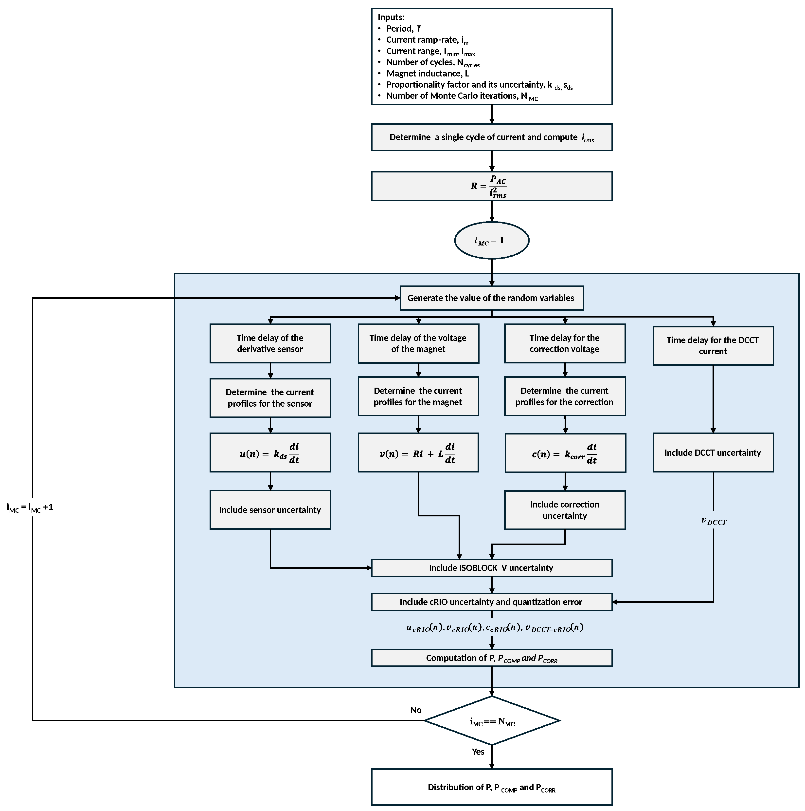
3.3. Simulation Setup

Figure 2 depicts the magnet model adopted in the present simulation. The inductance L is fixed to the best estimate available for magnet inductance, while the resistance R is retrieved from a power loss estimate. Notably, if $P_{ac}$ is the available estimate of AC power losses (e.g., obtained through FEM simulations), the resistance is obtained as $R=P_{ac}/I_{rms}^2$. Then, the voltage at the magnet terminal is

$$v\left(n\right)=Ri\left(n\right)+L{\displaystyle \frac{di}{dt}}\left(n\right)$$

(2)

A Monte Carlo simulation of the measurement was performed to validate the physical design of the instrument by estimating the measurement uncertainty in relevant conditions. The subject of the simulation was the quantity obtained according to (1), in its discrete form

$$P={\displaystyle \frac{1}{N}}\sum _{n=0}^{N-1}v\left(n\right)i\left(n\right),$$

(3)

where $v\left(n\right)$ are the samples of the measurand magnet voltage, $i\left(n\right)$ are the samples of the measurand magnet current, and N is the number of samples corresponding to an integer number of current cycles (i.e., periods of these waveforms). The sample rate was initially fixed to 1 kS/s to reduce the number of samples to simulate, but higher rates can be taken into account to achieve higher bandwidths for the measuring instrument.

In case of a correction or compensation of the magnet voltage, (3) is modified to

$$P_C={\displaystyle \frac{1}{N}}\sum _{n=0}^{N-1}\left[v\left(n\right)-u\left(n\right)\right]i\left(n\right),$$

(4)

where $u\left(n\right)$ are the samples of the inductive component of the magnet voltage that are calculated from the current samples or measured using the derivative sensor. It is worth noting that, ideally, $P=P_C$ given that the integration over an integer number of periods in (3) and (4) would in any case correspond only to the dissipated power. Nonetheless, due to the errors and uncertainties in the real scenario, the two power estimates can be significantly different.

The output voltage $u\left(n\right)$ of the derivative sensor is the sampled version of

$$u\left(t\right)=k_{ds}{\displaystyle \frac{di\left(t\right)}{dt}},$$

(5)

where $k_{ds}$ is a proportionality factor that could be an estimation of the magnet inductance or depend on the geometry and the core material in the case of the derivative sensor. In the latter case, the expression of $k_{ds}$ according to [37] is

$$k_{ds}={\displaystyle \frac{{\mu }_0{\mu }_r{A}_c{n}_2}{l_c+2{\mu }_r{l}_a}},$$

(6)

where ${\mu }_0$ is the free space magnetic permeability, ${\mu }_r$ is the relative permeability of the core material, $A_c$ is the cross-section area of the core, $n_2$ is the number of turns of the secondary (pick-up) coil, $l_c$ is the length of the magnetic path, and $l_a$ is the air gap length.

The uncertainty associated with the $k_{ds}$ must be also evaluated. To this aim, a nested Monte Carlo simulation was used. The starting point consisted of the uncertainties of quantities in (6). The flowchart of this simulation is shown in Figure 3. Ideally, the nominal values of the quantities in (6) should be selected to ensure $k_{ds}$ is equal to the magnet inductance; however, in practice, component tolerances prevent achieving an exact match, resulting in a deviation from the desired inductance. Hence, by sampling from the probability distributions associated with tolerances of each parameter, the tolerance of $k_{ds}$ can be retrieved. In a similar way, its uncertainty can be retrieved. The assumption was that each parameter had an uncertainty equal to a tenth of the respective tolerance. Both uncertainties and tolerances were thus considered in the simulation to understand the effect of unknown fluctuations as well as the influence of systematic deviations.

The flowchart of the Monte Carlo simulation for the entire measuring instrument is shown in Figure 4. The inputs for the simulation concern the supply current, the magnet model, and the correction mechanism. The input current waveform is defined by setting the period of a single cycle, the number of current cycles to simulate, the minimum and maximum current values, and the ramp rate. Such parameters allow the creation of the current samples $i\left(n\right)$. Moreover, the root mean square of current $I_{rms}$ and the current derivative can be computed.

Each element of the metrological chain is simulated considering its errors and uncertainties contribution. The contributions depend on the acquisition steps for the respective quantity and each Monte Carlo iteration corresponds to an observation of the inherent random variable. With this setup, the measurand voltage is affected by the isolation module and the acquisition board, while the current is affected by the DCCT and the acquisition board. For the computation of the compensated voltage, the current would also go through the derivative sensor. Instead, in the correction case, the current derivative is affected by filtering delay. Next, all the quantities undergo the quantization process. Then, the power is calculated for each Monte Carlo iteration according to (3) or (4). The results of all iterations are ensembled to obtain the statistical distribution of the simulated powers.

4. Instrument Validation

The design of the AC loss measuring instrument was validated through Monte Carlo simulation. Among the applications of interests, the DISCORAP magnet of the FAIR was taken into account as a case study because of the available reference information [8]. Nonetheless, the proposed simulation setup could be applied to other scenarios to evaluate the design uncertainty and evaluate its sources.

4.1. Case Study

Within the DISCORAP case study, the current waveform represented in Figure 5 was adopted for ramping the superconducting magnet. The current spans from 0 $\mathrm{k}$$\mathrm{A}$ to 3 $\mathrm{k}$$\mathrm{A}$ with a ramp rate of 2 $\mathrm{k}$$\mathrm{A}$ ${\mathrm{s}}^{-1}$ and $3.5$ $\mathrm{s}$ long plateaux. The period of this current waveform is 10 $\mathrm{s}$ with an $I_{rms}$ of $2.01$ $\mathrm{k}$$\mathrm{A}$. This waveform is a representative case of the current shapes used in scanning magnets, where the particle beam is bent at different angles to span an area.

For the magnet model, the inductance value is $L=22.5 \mathrm{m}\mathrm{H}$. This was reasonably assumed to be frequency independent and constant given the very low frequency of the current waveform, in accordance with previous works on AC losses [8,38]. Given the current waveform, the value of the dissipated power is related to the case of a 1 T/s ramp rate and a $1.5$ $\mathrm{T}$ dipole field. The AC power losses under the considered conditions are $P_{ac}=37.6 \mathrm{W}$ [8] and, therefore, the equivalent resistance modeling the losses is R = $9.284$ $\mathsf{\mu }$$\mathsf{\Omega }$. Since the dissipated power depends on the current, the model resistance changes with that. Hence, the simulation is rigorously valid only when applying the current waveform reported in Figure 5, but it could be repeated under other conditions of interest.

To compensate the inductive component of the magnet voltage, the derivative sensor [37] could have the parameter values summarized in

Table 1. Parameters of a suitable derivative sensor for voltage compensation.

Quantity	Symbol	Value
relative permeability (Vitroperm)	${\mu }_r$	$5\times {10}^3$
core cross section	$A_c$	$18\times {10}^{-4}$ ${\mathrm{m}}^2$
secondary turns	$n_2$	$2\times {10}^4$
air gap	$l_a$	$1\times {10}^{-3}$ $\mathrm{m}$
magnetic length in the core	$l_c$	$3\times {10}^{-1}$ $\mathrm{m}$

. This would result in $k_{ds}\approx$ $22.6$ $\mathrm{m}$$\mathrm{H}$. The uncertainty associated with that is retrieved by a further Monte Carlo simulation by considering about 10 $\mathsf{\mu }$$\mathrm{m}$ of 1 $\sigma$ uncertainty on the geometrical quantities. Meanwhile, component tolerances could lead to a systematic difference between $k_{ds}$ and L in the order of 10% (worst-case scenario). The introduced delay was assumed compatible with the DCCT one given the similar operation principle (order of $\mathsf{\mu }\mathrm{s}$).

If a numerical derivative is exploited instead of the derivative sensor, it is reasonable to assume a tolerance still in the order of 10%, while no uncertainty on the $k_{ds}$ value would be considered because this is exactly fixed in the correction calculations. Instead, a significant time delay would be introduced in this correction when numerically filtering the current to be derived. Previous research [37] suggested that about 250 $\mathrm{m}$$\mathrm{s}$ could be introduced as a time delay, which would be unacceptably large. This value is related to the order of the filter (250) and the sampling rate (1 kS/s). For instance, the delay could be reduced to 2.5 ms by reducing the order of the filter to 25 while increasing the sampling rate to 10 kS/s. Although feasible, such choices would deteriorate the signal-to-noise ratio while requiring more computational power in the measuring instrument (due to more samples). Moreover, preliminary simulations revealed that such a delay would still be too large.

The first analysis confirmed that the time delay introduces a misalignment between the magnet voltage and the correction voltage, which, in turn, affects the AC loss measurement. Given that the nominal time delay of the correction would be known once the filter order and the sample rate are set, the issue could be mitigated by introducing the same delay in the measured magnet voltage and current. The drawback would be to introduce a latency in the calculation of the overall dissipated power, but this could be acceptable for the real-time constraints of the application. Meanwhile, it is reasonable to assume that the correction delay value would still be affected by a 1% uncertainty, evaluated (in absence of further information) with a type B approach by relying on its resolution and previous experience. This contribution is reported in

Table 2. Uncertainty contributions due to the measurement chain for the power losses.

	Gain	Offset	Time Delay
DCCT	37 $\mathrm{ppm}$	−70 $\mathsf{\mu }$$\mathrm{V}$ to 70 $\mathsf{\mu }$$\mathrm{V}$	1 $\mathsf{\mu }$$\mathrm{s}$ to 5 $\mathsf{\mu }$$\mathrm{s}$
isolation module	−0.2% to 0.2%	−500 $\mathsf{\mu }$$\mathrm{V}$ to 500 $\mathsf{\mu }$$\mathrm{V}$	0 $\mathsf{\mu }$$\mathrm{s}$ to 5.7 $\mathsf{\mu }$$\mathrm{s}$
acquisition module	−0.03% to 0.03%	−842 $\mathsf{\mu }$$\mathrm{V}$ to 842 $\mathsf{\mu }$$\mathrm{V}$	200 $\mathsf{\mu }$$\mathrm{s}$ $\pm$ 1%
$k_{ds}$ (compensation)	0.63%	$\pm$10%	0 $\mathsf{\mu }$$\mathrm{s}$ to 6 $\mathsf{\mu }$$\mathrm{s}$
$k_{ds}$ (correction)		$\pm$10%	0.0 $\mathrm{m}$$\mathrm{s}$ to 0.2 $\mathrm{m}$$\mathrm{s}$
ADC quantization error: 24 bit

along with other uncertainty contributions, as detailed in Section 4.2.

4.2. Uncertainty Analysis

When not otherwise mentioned, the measurement uncertainties for the Monte Carlo analysis were retrieved from the technical specifications of the components according to the physical design and the case study. These are summarized in Table 2, which reports, for each element, the contribution in terms of gain, offset, and time delay. A uniform probability distribution was used whenever that contribution was reported as a range of values; otherwise, a normal probability distribution was adopted. This is compliant with the supplement of the guide to the expression of uncertainty in measurement [39]. The table also reports the values associated with $k_{ds}$ calculated with the nested Monte Carlo simulation, and the quantization error.

The Monte Carlo analysis was implemented in Python 3.12 and the code is publicly available (see Data Availability Statement). This fosters experiment reproducibility and customization to other case studies. In preliminary simulations, 500 to 100,000 Monte Carlo iterations were performed. Given that no significant difference was observed in results above 10,000, this number of iterations was considered in ensuing simulations as a compromise between computational burden and accuracy. The analyses were executed on an Intel^® Core™ i7-12700H (2.70 GHz CPU speed and 16 GB of RAM), and about 7 h was needed to complete the 10,000 iterations of the uncertainty analysis.

The normality was checked for the power loss distributions obtained with simulations. For this purpose, a chi-squared test with $\alpha$ = 5% significance was adopted. A histogram is reported in Figure 6 for the compensation scenario and a specific number of current cycles considered for the integration. In all the cases of interest, the null hypothesis for the normality test was that “the data do not follow a normal distribution”. The rejection of this hypothesis implied that the data are normally distributed, with a probability of a false statement of up to $\alpha$ = 5%. This justifies the synthetic description of the results in terms of the mean and variance.

Figure 7 shows the results of the Monte Carlo simulation for analyzing the uncertainties of the designed system. The considered scenarios concern a case with no compensation or correction (blue), a case of compensation by means of a derivative sensor (orange), and a case of correction relying on the numerical derivative of the current (green). The DISCORAP magnet power loss is also reported as a dashed line and it constitutes the ground truth. In the first case, the results point out that the mean AC losses equal about $37.6$ $\mathrm{W}$ with a 1 $\sigma$ uncertainty from 1.6 $\mathrm{W}$ to 0.2 $\mathrm{W}$ as more cycles are used for the integration.

In the two cases of compensation and correction, the 1 $\sigma$ uncertainty is higher, while the mean value converges to the ground truth value as the number of cycles increases in the compensation case only. In detail, for the compensation case, at least 20 cycles (200 $\mathrm{s}$ of acquisition) would be needed for a mean AC loss value settled at $37.5$ $\mathrm{W}$, with the 1 $\sigma$ uncertainty spanning from 5.6 $\mathrm{W}$ to 2.5 $\mathrm{W}$ in the 20 to 100 cycle range. For the correction case, the mean AC loss value converges to about 35 $\mathrm{W}$, while the 1 $\sigma$ uncertainty spans from 5.7 W to 2.9 W in the same 20 to 100 cycle range. Ultimately, the uncertainty analysis results suggest that the stated requirements for the AC loss measuring instrument would be almost reached only in the case of no compensation or correction. Section 4.3 will analyze the impact of the different uncertainty sources on the overall uncertainty by means of a sensitivity analysis. This will pave the way to improve the metrological characteristics of the proposed instrument, especially in the compensation and correction cases.

4.3. Sensitivity Analysis

Uncertainty sources were investigated through Monte Carlo simulation by considering one contribution at a time while zeroing the remaining ones. This approach is compliant with the “total effects analysis” [40], which aims to highlight the contribution of each single factor and its higher-order interactions with other factors. Given that the correction case was taken into account at this stage, the inherent contributions summarized in Table 2 were 11. They can be divided into four groups according to the respective element of the metrological chain (DCCT, isolation module, acquisition module, correction mechanism). Meanwhile, the ADC quantization error was never zeroed in the analyses.

Figure 8 reports the results of the analyses in terms of the standard deviation as a function of the number of cycles exploited in the integration. The four subplots correspond to the groups created according to the metrological chain elements. Then, in each subplot, the gain, offset, and time delay contributions are shown. These results suggest that the greatest contribution is from the offset of the $k_{ds}$ factor in the correction mechanism. The second contribution is from the time delay that is still associated with the correction mechanism. Similar contributions could be expected in the compensation case. However, while the offset contribution is in the same order of magnitude, it should be noted that the time delay is 100 times lower (Table 2). Other significant contributions would be related to the offset of the acquisition module and the gain of the isolation module. These would be also related to the uncertainty of the no compensation or correction cases.

Thanks to the sensitivity analysis results, the uncertainty analysis could be repeated to simulate a reduction in the main uncertainty contributions. First, only the offset uncertainty of the $k_{ds}$ was reduced to 1%. Next, the only time delay of the correction case was limited to $0.02$ $\mathrm{m}$$\mathrm{s}$, and these two results are reported in Figure 9. They demonstrate that reducing the offset uncertainty of the $k_{ds}$ leads to a lower standard deviation in the compensation case and in the correction case while not improving the error of the AC power losses in the correction case. Instead, the latter error is greatly reduced by acting on the time delay.

The last case taken into account was when the only offset uncertainty of the acquisition module was reduced to the $-84.2$ $\mathsf{\mu }$$\mathrm{V}$ to $84.2$ $\mathsf{\mu }$$\mathrm{V}$ range. This was especially carried out for the reduction of the uncertainty in the case of no compensation or correction, because the sensitivity analysis showed that the acquisition module offset is the highest contribution in that case. Figure 10 reports the results in terms of the only no compensation/correction case. They suggest that at least 20 cycles would be needed for a 1 $\sigma$ uncertainty equal to $0.2$ $\mathrm{W}$ and that $0.1$ $\mathrm{W}$ uncertainty can be reached at 100 cycles, with a mean AC loss value settled at the reference value of $37.6$ $\mathrm{W}$.

5. Conclusions

An AC power loss measuring instrument was designed and numerically validated for ramped superconducting magnets. This instrument was realized as part of the IRIS to comply with the requirements of various case studies. It allows the measurement of power losses, complementing magnet modeling. To this aim, system components were selected to fulfill the metrological requirements. A Monte Carlo analysis was performed to validate the design by evaluating the measurement uncertainty. Given the uncertainty analysis, the different contributions were also investigated by means of a sensitivity analysis. The AC power losses were investigated by considering different numbers of current cycles, which relate to different integration times in the measurement process.

The simulations demonstrate that AC power losses can be measured with the required accuracy without implementing any correction or compensation schemes. As expected, the measurement uncertainty decreases as the integration time increases. Moreover, the bottlenecks for higher metrological performance were pointed out even for the case of compensation and correction of the inductive magnet voltage component. The correction mechanism was thoroughly investigated due to its simpler implementation compared to the compensation, although they are theoretically equivalent. However, the errors and uncertainties of the numerical corrections were prohibitive to reaching the target accuracy, firstly due to uncertainties in modeling the magnet inductance.

Future studies will involve the on-field application of the proposed instrument, to measure the AC power losses on different magnets. For different case studies, the simulations can be reproduced to tailor the uncertainty analyses prior to the on-field measurements. Moreover, the Monte Carlo simulations also pave the way to further improvements to the designed instrument when the application requires it. By adopting the proposed methodology, the sensitivity analysis could also be extended to highlight their interactions in addition to the total effects.

References

1. Ang, Z.; Bejar, I.; Bottura, L.; Richter, D.; Sheahan, M.; Walckiers, L.; Wolf, R. Measurement of AC loss and magnetic field during ramps in the LHC model dipoles. IEEE Trans. Appl. Supercond. 1999, 9, 742–745. [Google Scholar] [CrossRef]
2. Di Castro, M.; Bottura, L.; Richter, D.; Sanfilippo, S.; Wolf, R. Coupling current and AC loss in LHC superconducting quadrupoles. IEEE Trans. Appl. Supercond. 2008, 18, 108–111. [Google Scholar] [CrossRef]
3. Hatanaka, K.; Nakagawa, J.; Fukuda, M.; Yorita, T.; Saito, T.; Sakemi, Y.; Kawaguchi, T.; Noda, K. A HTS scanning magnet and AC operation. Nucl. Instruments Methods Phys. Res. Sect. Accel. Spectrometers Detect. Assoc. Equip. 2010, 616, 16–20. [Google Scholar] [CrossRef]
4. Fischer, E.; Schnizer, P.; Sugita, K.; Meier, J.P.; Mierau, A.; Bleile, A.; Szwangruber, P.; Müller, H.; Roux, C. Fast-ramped superconducting magnets for FAIR production status and first test results. IEEE Trans. Appl. Supercond. 2015, 25, 4003805. [Google Scholar] [CrossRef]
5. Amano, S.; Takayama, S.; Orikasa, T.; Nakanishi, K.; Hirata, Y.; Iwata, Y.; Mizushima, K.; Abe, Y.; Noda, E.; Urata, M.; et al. Thermal design and test results of the superconducting magnet for a compact heavy-ion synchrotron. IEEE Trans. Appl. Supercond. 2022, 32, 4401305. [Google Scholar] [CrossRef]
6. Vulusala G, V.S.; Madichetty, S. Application of superconducting magnetic energy storage in electrical power and energy systems: A review. Int. J. Energy Res. 2018, 42, 358–368. [Google Scholar] [CrossRef]
7. Ozelis, J.; Delchamps, S.; Gourlay, S.; Jaffery, T.; Kinney, W.; Koska, W.; Kuchnir, M.; Lamm, M.; Mazur, P.; Orris, D.; et al. AC loss measurements of model and full size 50 mm SSC collider dipole magnets at Fermilab. IEEE Trans. Appl. Supercond. 1993, 3, 678–681. [Google Scholar] [CrossRef]
8. Volpini, G.; Alessandria, F.; Bellomo, G.; Fabbricatore, P.; Farinon, S.; Gambardella, U.; Manfreda, G.; Musenich, R.; Quadrio, M.; Sorbi, M. AC losses measurement of the DISCORAP model dipole magnet for the SIS300 synchrotron at FAIR. IEEE Trans. Appl. Supercond. 2013, 24, 4000205. [Google Scholar] [CrossRef]
9. Felcini, E.; Pullia, M.; Sabbatini, L.; Vannozzi, A.; Trigilio, A.; Pivi, M.; De Cesaris, I.; Rossi, L.; Prioli, M.; Schwarz, P.; et al. Characterization of hysteretic behavior of a FeCo magnet for the design of a novel ion gantry. IEEE Trans. Appl. Supercond. 2024, 34, 4402105. [Google Scholar] [CrossRef]
10. Yang, Y.; Matsuba, S.; Mizushima, K.; Fujimoto, T.; Iwata, Y.; Noda, E.; Urata, M.; Shirai, T.; Nishijima, G.; Takayama, S.; et al. Design and test of a 0.4-m long short model of a conduction-cooled superconducting combined function magnet for a compact, rapid-cycling heavy-ion synchrotron. Nucl. Instruments Methods Phys. Res. Sect. Accel. Spectrometers Detect. Assoc. Equip. 2023, 1050, 168165. [Google Scholar] [CrossRef]
11. Karppinen, M.; Ferrentino, V.; Kokkinos, C.; Ravaioli, E. Design of a curved superconducting combined function bending magnet demonstrator for hadron therapy. IEEE Trans. Appl. Supercond. 2022, 32, 4400705. [Google Scholar] [CrossRef]
12. Marchevsky, M. Quench detection and protection for high-temperature superconductor accelerator magnets. Instruments 2021, 5, 27. [Google Scholar] [CrossRef]
13. Zhang, H.; Wen, Z.; Grilli, F.; Gyftakis, K.; Mueller, M. Alternating current loss of superconductors applied to superconducting electrical machines. Energies 2021, 14, 2234. [Google Scholar] [CrossRef]
14. Ashworth, S.; Suenaga, M. Local calorimetry to measure ac losses in HTS conductors. Cryogenics 2001, 41, 77–89. [Google Scholar] [CrossRef]
15. Ghoshal, P.; Coombs, T.; Campbell, A. Calorimetric method of ac loss measurement in a rotating magnetic field. Rev. Sci. Instruments 2010, 81, 074702. [Google Scholar] [CrossRef]
16. Wilson, M. Superconducting Magnets; Monographs on cryogenics; Clarendon Press: Oxford Science Publications, UK, 1983. [Google Scholar]
17. Willering, G. Loss measurements in superconducting magnets at CERN. In Proceedings of the HFM Meeting, Zurich, Switzerland, 26 September 2024. [Google Scholar]
18. Li, X.; Ren, L.; Guo, S.; Xu, Y.; Shi, J.; Tan g, Y.; Li, J. A novel AC loss measurement method for HTS coils based on parameter identification. Supercond. Sci. Technol. 2022, 35, 065021. [Google Scholar] [CrossRef]
19. Verweij, A.; Leroy, D.; Walckiers, L.; Wolf, R.; Ten Kate, H. Analysis of the AC loss measurements on the one-metre dipole model magnets for the CERN LHC. IEEE Trans. Magn. 1994, 30, 1758–1761. [Google Scholar] [CrossRef]
20. Yuan, W.; Coombs, T.; Kim, J.H.; Han Kim, C.; Kvitkovic, J.; Pamidi, S. Measurements and calculations of transport AC loss in second generation high temperature superconducting pancake coils. J. Appl. Phys. 2011, 110. [Google Scholar] [CrossRef]
21. Shen, B.; Li, C.; Geng, J.; Zhang, X.; Gawith, J.; Ma, J.; Liu, Y.; Grilli, F.; Coombs, T. Power dissipation in HTS coated conductor coils under the simultaneous action of AC and DC currents and fields. Supercond. Sci. Technol. 2018, 31, 075005. [Google Scholar] [CrossRef]
22. Zhu, K.; Guo, S.; Ren, L.; Xu, Y.; Wang, F.; Yan, S.; Liang, S.; Tang, Y.; Shi, J.; Li, J. AC loss measurement of HTS coil under periodic current. Phys. Supercond. Appl. 2020, 569, 1353562. [Google Scholar] [CrossRef]
23. Šouc, J.; Pardo, E.; Vojenčiak, M.; Gömöry, F. Theoretical and experimental study of AC loss in high temperature superconductor single pancake coils. Supercond. Sci. Technol. 2008, 22, 015006. [Google Scholar] [CrossRef]
24. Liao, Y.; Tang, Y.; Shi, J.; Shi, X.; Ren, L.; Li, J.; Wang, Z.; Xia, Z. An automatic compensation method for measuring the AC loss of a superconducting coil. IEEE Trans. Appl. Supercond. 2016, 26, 9001805. [Google Scholar] [CrossRef]
25. De Bruyn, B.; Jansen, J.; Lomonova, E. AC losses in HTS coils for high-frequency and non-sinusoidal currents. Supercond. Sci. Technol. 2017, 30, 095006. [Google Scholar] [CrossRef]
26. Breschi, M.; Macchiagodena, A.; Ribani, P.L.; Bellina, F.; Stacchi, F.; Bermudez, S.I.; Bajas, H. Experimental and Numerical Investigation on Losses in Electrodynamic Transients in a Nb3Sn Prototype Racetrack Coil. IEEE Trans. Appl. Supercond. 2018, 28, 4000605. [Google Scholar] [CrossRef]
27. Rossi, L.; Arpaia, P.; Attanasio, C.; Avallone, G.; Avitabile, F.; Balconi, L.; Bellingeri, E.; Beneduce, E.; Benson, T.; Bernini, C.; et al. IRIS-a new distributed research infrastructure on applied superconductivity. IEEE Trans. Appl. Supercond. 2023, 34, 9500309. [Google Scholar] [CrossRef]
28. Rossi, L.; Balconi, L.; Campana, P.; Felis, S.M.; Sorti, S.; Statera, M. IRIS—The Italian research infrastructure on Applied Superconductivity for Particle Accelerators and Societal Applications. J. Phys. Conf. Ser. 2024, 2687, 092012. [Google Scholar] [CrossRef]
29. Fabbricatore, P.; Alessandria, F.; Bellomo, G.; Farinon, S.; Gambardella, U.; Kaugerts, J.; Marabotto, R.; Musenich, R.; Moritz, G.; Sorbi, M.; et al. Development of a curved fast ramped dipole for FAIR SIS300. IEEE Trans. Appl. Supercond. 2008, 18, 232–235. [Google Scholar] [CrossRef]
30. De Matteis, E.; Barna, D.; Ceruti, G.; Kirby, G.; Lecrevisse, T.; Mariotto, S.; Perini, D.; Prioli, M.; Rossi, L.; Scibor, K.; et al. Straight and curved canted cosine theta superconducting dipoles for ion therapy: Comparison between various design options and technologies for ramping operation. IEEE Trans. Appl. Supercond. 2023, 33, 4401205. [Google Scholar] [CrossRef]
31. Prioli, M.; De Matteis, E.; Farinon, S.; Felcini, E.; Gagno, A.; Mariotto, S.; Musenich, R.; Pullia, M.; Rossi, L.; Sorbi, M.; et al. Design of a 4 T Curved Demonstrator Magnet for a Superconducting Ion Gantry. IEEE Trans. Appl. Supercond. 2023, 33, 1–5. [Google Scholar] [CrossRef]
32. Toral, F.; Barna, D.; Calzolaio, C.; Carloni, A.; Ceruti, G.; De Matteis, E.; Kirby, G.; Lecrevisse, T.; Mariotto, S.; Munilla, J.; et al. Status of Nb-Ti CCT Magnet EU Programs for Hadron Therapy. IEEE Trans. Appl. Supercond. 2024, 34, 4401705. [Google Scholar] [CrossRef]
33. De Matteis, E.; Ballarino, A.; Barna, D.; Carloni, A.; Echeandia, A.; Kirby, G.; Lecrevisse, T.; Lucas, J.; Mariotto, S.; van Nugteren, J.; et al. Conceptual Design of an HTS Canted Cosine Theta Dipole Magnet for Research and Hadron Therapy Accelerators. IEEE Trans. Appl. Supercond. 2024, 34, 4402505. [Google Scholar] [CrossRef]
34. Levi, F.; Bersani, A.; Bianchi, E.; Carloni, A.G.; Cereseto, R.; De Matteis, E.; Farinon, S.; Felcini, E.; Gagno, A.; Georgiadis, G.; et al. Mechanical Design of the 4 T Curved Demonstrator Dipole for the SIG Gantry. IEEE Trans. Appl. Supercond. 2024, 34, 4400505. [Google Scholar] [CrossRef]
35. Steckert, J.; Kopal, J.; Bajas, H.; Denz, R.; Georgakakis, S.; De Matteis, E.; Spasic, J.; Siemko, A. Development of a digital quench detection system for nb 3 Sn magnets and first measurements on prototype magnets. IEEE Trans. Appl. Supercond. 2018, 28, 4703304. [Google Scholar] [CrossRef]
36. Courts, S.S.; Swinehart, P.R. Review of Cernox™(Zirconium Oxy-Nitride) Thin-Film Resistance Temperature Sensors. In Proceedings of the AIP Conference Proceedings. American Institute of Physics, Chicago, IL, USA, 21–24 October 2022; Volume 684, pp. 393–398. [Google Scholar] [CrossRef]
37. De Matteis, E.; Calcoen, D.; Denz, R.; Siemko, A.; Steckert, J.; Storkensen, M. New method for magnet protection systems based on a direct current derivative sensor. IEEE Trans. Appl. Supercond. 2018, 28, 4700505. [Google Scholar] [CrossRef]
38. Kim, J.H.; Kim, C.H.; Iyyani, G.; Kvitkovic, J.; Pamidi, S. Transport AC loss measurements in superconducting coils. IEEE Trans. Appl. Supercond. 2010, 21, 3269–3272. [Google Scholar] [CrossRef]
39. BIPM; IEC; IFCC; ILAC; ISO; IUPAC; IUPAP; OIML. Evaluation of measurement data—Supplement 1 to the “Guide to the expression of uncertainty in measurement” —Propagation of distributions using a Monte Carlo method. Jt. Comm. Guid. Metrol. 2008, 111, 17. [Google Scholar] [CrossRef]
40. Saltelli, A. Global Sensitivity Analysis: The Primer; John Wiley & Sons: Hoboken, NJ, USA, 2008. [Google Scholar] [CrossRef]
Figure 1. Architecture of the AC loss measuring instrument.
Instruments 09 00008 g001
Figure 2. Simple electrical model of a magnet from the perspective of power loss measurements.
Instruments 09 00008 g002
Figure 3. Flowchart of the nested Monte Carlo simulation used to evaluate the k d s , its associated tolerance t d s , and uncertainty s d s .
Instruments 09 00008 g003
Figure 4. Flowchart of the Monte Carlo simulation. White boxes represent inputs and outputs, while gray boxes highlight computations.
Instruments 09 00008 g004
Figure 5. Current waveform adopted in current analysis as retrieved from the case study [8].
Instruments 09 00008 g005
Figure 6. Histogram of AC loss values obtained with 100 current cycles when the compensation mechanism is used.
Instruments 09 00008 g006
Figure 7. Results of the simulated AC power losses as a function of current cycles in the cases of no compensation/correction, compensation through a derivative sensor, and correction through a numerical derivative. The reference AC power loss of the case study is also reported as the ground truth.
Instruments 09 00008 g007
Figure 8. Results of the sensitivity analysis for the AC power loss uncertainty contributions reported as standard deviations in the function of current cycles.
Instruments 09 00008 g008
Figure 9. Results of the simulated AC power losses obtained after reducing by 10 times (a) the offset of the k d s factor and (b) the time delay from the correction mechanism as highlighted by the sensitivity analysis.
Instruments 09 00008 g009
Figure 10. Results of the simulated AC power losses obtained without compensation or correction after reducing by 10 times the offset of the acquisition module.
Instruments 09 00008 g010