1. Introduction
Optical beam-loss monitors (oBLM) have become increasingly widespread as distributed beam-loss monitoring systems since their first development in 2000 [
1,
2,
3,
4,
5,
6]. They consist of a multimode optical fibre with photosensors attached at either or both sides of the fibre. The fibre is typically placed parallel and as close as possible to the beamline, while the photosensors are located in more shielded areas. Whenever beam losses occur, charged particles above a certain threshold velocity traversing the optical fibre induce Cherenkov radiation [
7]. A proportion of these photons can be captured by the optical fibre, propagated to the fibre ends, and read out by the photosensors [
8]. The optical fibre acts not only as a detecting medium but is also used to transport the measured signal to the readout, allowing for some flexibility in the exact location of the photosensors. The signal amplitude then gives the intensity of the beam loss, while the time of arrival of the pulse indicates the loss position.
Previously, multiple studies on oBLMs have been conducted, both at CERN [
9,
10], and at other accelerators around the world [
2,
3,
4,
5,
6]. Fibre thicknesses between 200 μm and 1 mm and fibre lengths up to 200 m have been studied [
2,
4,
5,
9]. Although most installations attached silicon photomultipliers (SiPMs) to the upstream end of the fibre, some studies chose to instead use photomultiplier tubes (PMTs) attached to the downstream end of the fibre [
4,
5,
9]. SiPMs and PMTs are the only detectors suitable for the low signal levels in the order of single photons. While SiPMs are typically notably cheaper, mechanically robust, and need lower operational voltages, PMTs can be significantly more radiation-hard and have a lower amount of dark counts [
11,
12].
These studies have found multiple advantages of oBLMs compared to other beam-loss detection systems. Typically, point-like detectors such as diamond, scintillation, or ionisation chamber detectors are used. Compared to these, the main advantage of oBLMs is the large longitudinal coverage, minimising the number of detectors needed to cover large accelerators. The main direct alternative to oBLMs are long ionisation chambers which can also be used to cover large distances of 100 m. However, these signals are typically significantly slower (timescale of 100 ms) and noisier than oBLMs [
4,
5].
In the following, a novel installation at the CERN Linear Electron Accelerator for Research (CLEAR) will be introduced. This setup builds upon the previously installed prototype, presented in [
9], which used two shorter fibres, one for each readout. This installation instead uses a single fibre and extends the fibre to cover the entire accelerator. Furthermore, a constant vertical distance between the fibre and the beam pipe is ensured by using optical posts. The installation has been augmented by Monte-Carlo simulations, which are presented and discussed in the following. These give a better understanding of the expected loss-shower particle distributions. Furthermore, to the best of our knowledge, both SiPMs and PMTs were tested at the same installation for the first time. This enables a direct comparison between the two photon-detector types and the measured loss signals. This comparison was conducted with multiple methods of signal analyses and loss-position-reconstruction techniques. These analysis methods have previously not been compared for oBLMs and it will be shown how the accuracy of such an installation can be increased without needing to adjust the installation itself.
2. Materials and Methods
After promising results with a prototype setup at CLEAR [
9], it was decided to install a permanent oBLM, covering the entire length of the accelerator. This new setup should help visualise beam losses along the accelerator and thereby help with daily beam operations. Especially when changing beam energies or when restarting the accelerator, adjustments to the magnet system have to be made to ensure the beam is being fully transported to the beam dump. Knowing precisely where the beam is lost can indicate which magnets to adjust accordingly, which can significantly decrease time needed for setting up the beam and thus increase the effective beam time available for users.
2.1. CLEAR
CLEAR is a ∼40 m long linear electron accelerator at CERN. It consists of a 20 m long accelerating section, split into three structures, followed by a 20 m long experimental beam line. As visualised in
Figure 1, CLEAR can generate and accelerate a beam train up to ten times per second. Each beam train consists of up to 150 bunches which are spaced by 333 ps or 666 ps. The bunch charge can be adjusted from 10 pC to
nC per bunch [
13]. Furthermore, the beam energies can range from 60 MeV to 220 MeV. For the following measurements, a bunch spacing of 666 ps, a train repetition rate of
Hz, and a beam energy of 200 MeV were used. These beam settings are used to investigate, amongst others, plasma lens and THz acceleration, medical applications of electron beams, and various types of beam instrumentation [
14,
15].
2.2. oBLM
For this installation, a 200 μm thick, 130 m long ‘FG200LEA’ optical fibre from Thorlabs with low hydroxyl ion concentration was installed [
16]. This length was chosen to shield the readout electronics from radiation by placing them in the gallery above the accelerator, as visualised in
Figure 2. The thickness had been experimentally verified previously to be sufficient [
9]. Along the accelerator, optical posts were used to ensure a constant vertical distance of 45 cm to the middle of the beam pipe. This was the minimum distance possible due to other beam instrumentation along the beam line. This specific fibre was chosen as it shows the lowest attenuation over the wavelength range of interest for Cherenkov radiation. Photosensors, S14160-3010PS SiPMs and R9880U-116 PMTs from Hamamatsu, were investigated due their high photon-detection efficiency over the wavelength range of interest which is a convolution of the initial Cherenkov distribution and the wavelength and distance-dependent attenuation within the fibre [
17,
18].
3. FLUKA Simulations
To fully understand the expected loss signals, a number of simulations were conducted in the particle-physics Monte-Carlo simulation package FLUKA [
19,
20,
21]. For these simulations, a simple geometry was chosen. It consists of a 220 MeV electron beam inside a 2 mm thick copper beam pipe with an inner radius of 2 cm, consistent with the values at CLEAR. The optical fibre was modelled as a 2 mm thick silica cylinder at a distance of 45 cm to the beam. This is a factor 10 increase over the true optical fibre diameter at 200 μm and was necessary to increase the capture factor of secondary particles for simulations to converge in a timely manner. A 1 cm thick copper target was placed in the beam trajectory to induce beam-loss showers.
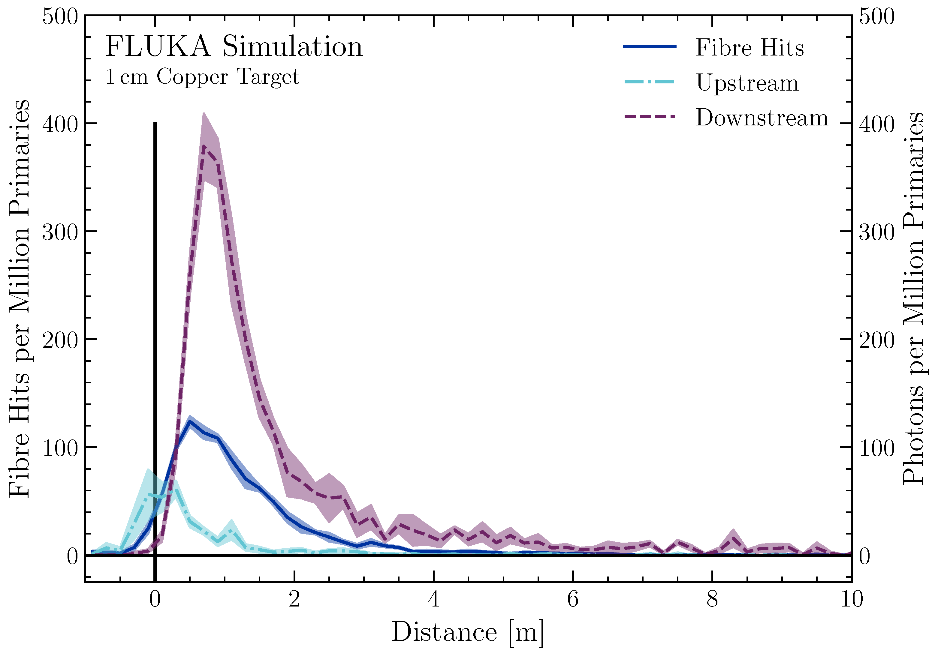
The simulations were run with 2.5 million primary electrons which create, on average, 1.5 secondary charged particles per primary with velocities above the threshold needed to generate Cherenkov radiation within the fibre. The loss-shower distribution is visualised in
Figure 3. Each of the dashed black lines visualises a particle hitting the fibre. For this setup with a distance between the fibre and the beam axis of 45 cm, 95% of fibre hits occur in the range −0.3 m to 4.7 m relative to the copper block; the maximum is located at 50 cm. Nevertheless, in this simulation run, 1% of fibre hits occur more than 15 m downstream of the copper block position.
A custom user routine was written to save the particle trajectories of the small fraction of the secondary particles which traverse the optical fibre. Furthermore, a python script was then used to convert these trajectories into the number of generated and captured Cherenkov photons in a wavelength range of 200 nm to 900 nm. Photons within the fibre only undergo total reflection, and therefore transport, within a certain angular range, depending on the numeric aperture of the fibre. As the angle under which charged particles emit Cherenkov photons is a function of velocity, only secondary particles traversing the fibre at certain angle–velocity combinations emit capturable photons [
8,
22]. For this fibre with a numeric aperture of 0.22, particles traversing the fibre at effectively the speed of light in vacuum in an angular range of 39° to 55° have a chance to emit captured photons in one direction. For further details on the simulations, the reader is referred to [
9]. The number of fibre hits and captured photons as a function of distance along the beam trajectory to the impact point on the copper block is given in
Figure 4.
Multiple features are visible in this plot. The downstream signal is notably higher than the number of fibre hits, which itself is greater than the number of photons which are captured and transported upstream. The upstream signal is smaller than the downstream signal due to the directionality of the loss shower and the limited capture angle of photons within the fibre. Only approximately a third of the charged particles hitting the fibre emit photons which are captured and transported downstream. For the upstream case, only roughly 5%—six times less than downstream—of particles hitting the fibre induce a signal which can be captured. Despite most fibre hits not emitting captured photons, one can see that, on average, a single fibre hit induces multiple captured photons; for this simulation, this equates to approximately three photons per charged particle impacting the fibre. As the number of generated Cherenkov photons is proportional to the distanced travelled by charged particles within the fibre, the number of captured photons per particle hit is expected to be significantly less for thinner fibres.
The backscattered fibre hits can be detected by measuring the upstream signal, light blue in
Figure 4, while the downstream signal, red, is induced mainly by particles hitting the fibre after the copper block. This, again, can be explained by the capture angle of photons within the fibre and the directionality of the loss particles. Overall, the downstream signal gives a much higher signal, which could be especially useful when detecting low amounts of beam losses.
4. Loss Position Reconstruction
To be able to measure the accuracy of the setup, beam losses were induced at known positions along the beam line. At CLEAR, this could be achieved by inserting beam screens in the beam line or by using kicker magnets to divert the beam into the beam pipe. When using kicker magnets, the loss shower is not created at the location of the magnets themselves but more than 1 m further downstream. The exact location is not only a function of the beam energy and magnet current but also of the exact beam position and angle. Due to this increased uncertainty, it was decided to neglect measurements with losses induced by kicker magnets for the position-reconstruction investigations.
In total, six screens can be inserted along the beam line at CLEAR. However, the beam does not reach its maximum energy until after the first screen. Also, the very end of the beam line, including the last screen, could not be covered by the fibre due to the beam dump location and size. This leaves four screens available for this investigation, BTV0390 at m, BTV0620 at m, BTV0730 at m, and BTV0810 at m. Screen BTV0620 is a 400 μm thick optical transition radiation (OTR) silicon screen; all other screens are 200 μm yttrium aluminium garnet (YAG) screens.
Losses were created at each of these screens, with trains consisting of 5, 10, 30 and 50 bunches to cover a wide range of train charges. The average bunch charge remained consistent at nC (1.9 × 10⁹ e−) for all bunch numbers. For each train configuration, 20 detector signals were recorded. For the case of 5 bunch trains, where the lowest signals are recorded, the standard deviation on the peak height, among the 20 signals, was found to be up to 20%. This uncertainty stems from shot-by-shot fluctuations of the beam intensity as well as the statistical nature of the loss-shower generation and scattering effects, the photon signal generation, capture, attenuation, and detection by the photon detectors, including the noise of these detectors and signal readout. By recording 20 signals, the standard error on the peak height can be reduced to below 5%. During operation, however, even single beam-train measurements can give valuable information on the loss position as the position of the maximum and rising edge fluctuates significantly less, as will be shown in the following, reducing the measurement time notably.
4.1. Signal Readout Considerations
Both ends of the fibre are attached to readout boards with photodetectors to save both the up- and downstream waveforms simultaneously. This is achieved by using an external trigger provided by the electron gun of the accelerator. Depending on the use case, using either or both fibre ends may be preferable. From the simulations discussed earlier, the measured downstream signal is expected to be much greater than the upstream signal by nearly one order of magnitude.
However, it can be easier to resolve signals from different loss locations when using the upstream waveform. This can be best visualised by investigating the signal paths from two loss positions
and
with a certain distance
, as shown in
Figure 5. At the upstream detector, the loss signal from
will arrive slightly after the loss signal from
with the difference in arrival time
between these two signals consisting of two parts. The first part corresponds to the time that the beam needs to cover the distance between the two loss locations. The second part corresponds to the time that the photons need to propagate along the fibre from the second loss location back to the first. Approximating the speed of the beam with the speed of light in vacuum,
c, and the speed of light in the fibre
with a refractive index
, this gives:
When considering the timing difference for the same two loss positions but for the downstream signal, these two parts are now opposing each other as the overall distance of the beam and signal remains the same, regardless of the loss location. For
, the distance
is covered by the photon signal within the fibre travelling at a speed of
. For
, this distance is covered by the beam at the speed of light. This means that the two parts of the formula above must be subtracted from each other:
One can now see that the measured time difference at the downstream sensor contains a scaling factor of ≈−0.5, i.e., signals will be measured closer and inverted in time. This is much lower than the upstream scaling factor of ≈2.5. This indicates that from a position resolution point of view, using the upstream signal should be better, assuming enough signal can be captured. With a given sampling frequency, the time difference between the two loss signal peaks will have many more resolvable data points for the upstream readout.
The final option is to subtract the time information from the two signals, which eliminates the need to time the two signals to a common, external trigger such as the electron gun. Instead, one can trigger on either of the signals and the time difference to the other signal can then be used to extract the loss location. This method, in theory, also removes the need for a position calibration, as the middle of the fibre is exactly when both signals arrive at the same time. In this case, the location along the fibre
x, with
being the upstream end of the fibre, is given by:
However, with an uncertainty on the length of 1%, i.e., m, given by the producer, as well as a notable uncertainty on the calibration between the fibre middle and the accelerator coordinate system, in practice it is often easier and more precise to simply conduct an offset calibration as for the other readout methods.
4.2. Investigated Conversion Methods
Apart from which fibre end to use, the other main consideration for loss position reconstruction is how to extract a timestamp to convert into a loss position from the measured waveform.
4.2.1. Peak Position
The most straightforward method is to take the time of the maximum of the waveform. With the external trigger triggering on the start of the beam train and the timing of the peak being shifted by approximately half of the train length due to the rise and fall time of the detectors, it was decided to subtract half the train length from this time to compensate for this effect. This was only carried out for this method.
4.2.2. Constant Threshold
Another simple method is to apply a constant threshold to all waveforms and then use the first time the signal rises above this level as the loss time. In this case, a value of 15 mV was chosen as the threshold.
4.2.3. Constant Fraction Discrimination
As a large range of beam-train charges are used during day-to-day operations, the loss signal amplitude is expected to vary significantly. One method to minimise the impact of these fluctuations is to use a constant fraction discrimination (CFD). For each waveform, a threshold is set at a fraction of the maximum signal. In this case, after testing multiple values, it was found that a fraction of 40% is the most consistent.
4.2.4. Gradient
Finally, the derivatives of the signals were investigated. While for high signals for the SiPMs, this method seemed promising [
10], the rising edge of the PMTs were too noisy and thus the derivative fluctuated greatly, leading to very high position uncertainties. Using a moving average can reduce this effect. Despite this, there did not seem to be a threshold value suitable for all screens and beam charges. Therefore, this method will be neglected in the following.
4.3. Loss Waveforms
In
Figure 6 and
Figure 7, mean example waveforms are shown for losses created by thirty bunches for the upstream and downstream ends respectively, measured with a PMT at 700 V. In these figures, the variance between different signals is visualised by the transparent band. The different time and signal scales between the figures is to be noted with the downstream signals being notably higher but closer in time, as expected from previous considerations.
In general, the different loss positions show differing signal heights. While the total beam loss should be similar for all waveforms, the instrumentation around the beam line in different locations differs significantly, which could lead to local shielding effects and thus reduce the measurable signal. This is a general issue when it comes to beam-loss monitors as often the ideal location, in this case immediately outside the beam pipe, is not accessible. Apart from this, slight changes in the beam trajectory can also have an impact on the loss-shower propagation, which can lead to fluctuations in the measured beam loss due to the extremely small angular coverage of the fibre. Calculating this coverage for the 2D case gives a percentage coverage of % of . Furthermore, the signal ratio between the upstream and downstream signals is now slightly larger than expected from simulations. This is attributed to the backscattering of secondary particles on the surrounding devices, leading to a relative increase in the measured upstream signal.
The downstream waveforms all clearly show a plateau with a width which corresponds to the train length of
ns. This behaviour is not visible for the upstream waveforms which seem to follow more the signal shape of the loss distribution simulation shown in
Figure 4. This is to be expected as a time difference equates to a much larger position difference downstream compared to upstream, as discussed previously. A 20 ns time spread upstream corresponds to a position difference of
m, whereas this same time spread corresponds to a position difference of 12 m downstream. This means that, for this specific case, the train length is the dominant factor for the downstream signal spread, whereas the loss shower distribution is the dominant factor for the upstream signal spread. For lower bunch numbers per train, this behaviour is not as dominant and the downstream peaks become notably sharper.
The upstream waveforms show two additional peaks besides the initial four, which correspond to the inserted beam screens, at 350 ns and 750 ns. These peaks can be seen for all measured waveforms, regardless of the inserted screen. The first of these peaks at 350 ns indicates a secondary loss location towards the end of the beam line. However, this peak is not visible when retracting all screens and transporting the beam through the entire beam line. Furthermore, the reconstructed position corresponds to a region in which the fibre is being led away from the beam line towards the readout and is no longer parallel to the beam line. This suggests that some particles from the loss showers hit the fibre at this location and, due to the changed angle, each particle potentially induces a relatively high signal, leading to a small peak at this location. This behaviour is still under investigation.
The signal at 750 ns, on the other hand, is well understood. The time difference between these signals and those measured downstream corresponds exactly to the time needed for photons to traverse the entire fibre. This indicates that these signals represent simply a reflection of the downstream signals at the downstream readout. A similar peak would, in theory, be expected downstream due to reflections from the upstream signals. However, as the downstream signals are much greater than the upstream signals, these signals are not expected to be resolvable above the noise.
Apart from these waveforms, different voltages (500, 700, 900 and 1000 V) were applied to the PMTs, greatly altering the typical gain from a factor of five thousand to two million. The expected increase in signal was visible and caused a saturation of the used data readout for trains with multiple bunches. Applying a high voltage of 1000 V did, however, enable measuring signals from beam losses down to a few pico-coulomb. Besides the increase in sensitivity, dark counts became increasingly visible for voltages above 900 V, which could significantly affect position-reconstruction algorithms for low signals. In these cases, it might become necessary to apply more elaborate techniques, such as averaging or fitting the signal peaks, when determining the true loss position.
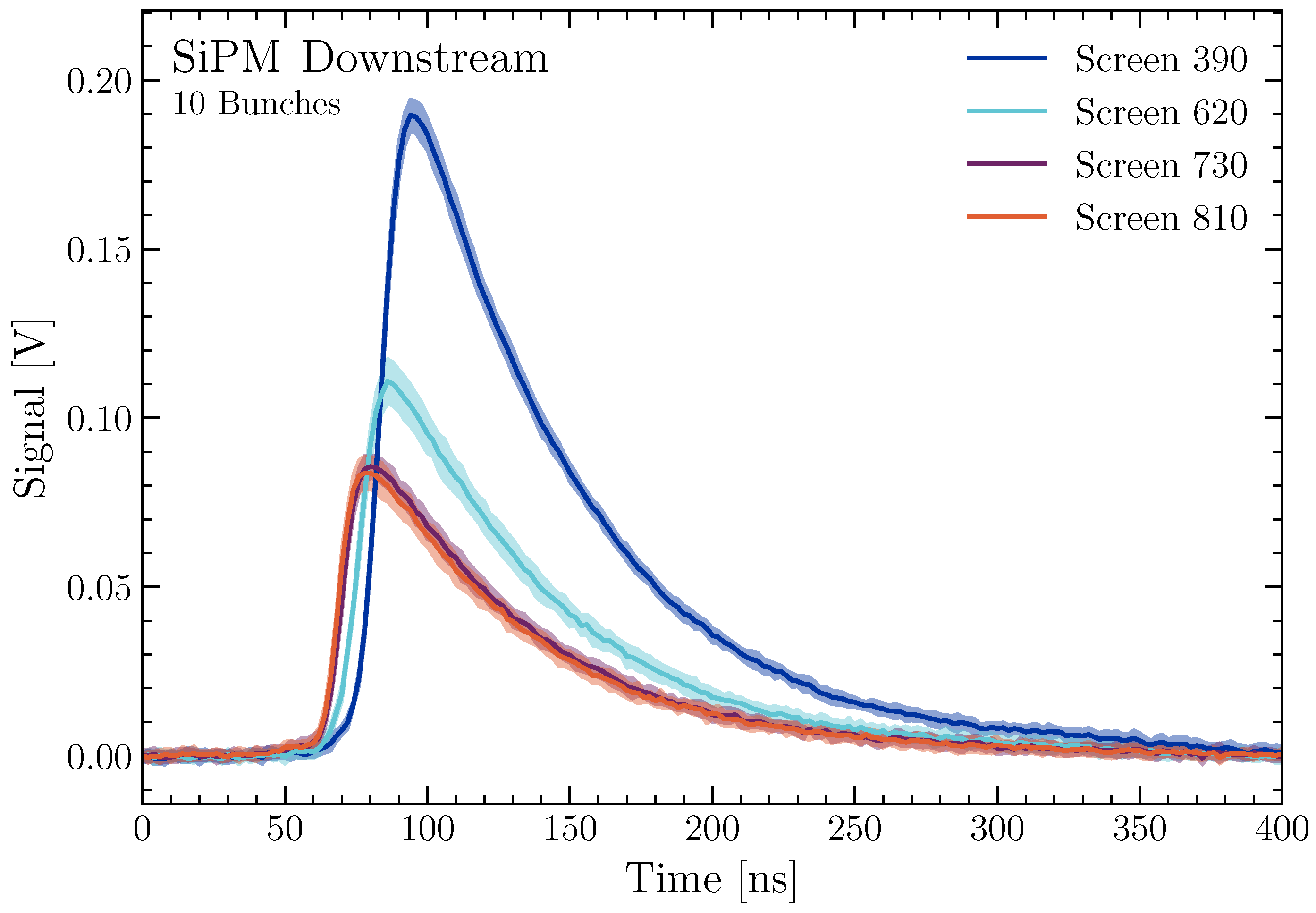
The same measurement conducted with the PMTs was also conducted with SiPMs and the corresponding upstream and downstream signals are given in
Figure 8 and
Figure 9, this time for a beam with ten bunches instead of thirty. This value was chosen to better visualise the statistical fluctuations on the SiPMs, especially for the upstream signal. With increasing signal height, the relative uncertainty decreases. At these applied voltages, the SiPMs show noise levels of 17 mV, while the noise is double that for the PMTs at 35 mV. When contrasting the signals recorded by the PMTs with those from the SiPMs, the most striking effect is the slightly longer rise time and notably longer fall time of the signals. While this is not a major issue for single losses, it is expected to be more difficult to resolve multiple loss locations with SiPMs in general [
11].
4.4. Analysis
To quantify the accuracy of the multitude of combinations between the photon detector (SiPM or PMT), fibre readout side (up- or downstream or combined) and signal-to-timestamp conversion (peak position, constant threshold or CFD), the loss waveforms measured at the four screens and for the four different numbers of bunches were converted into longitudinal positions for all combinations. To compute these loss position values and their uncertainties, the mean and standard deviation from the 20 measured waveforms, i.e., the 20 shot-by-shot loss measurements, were used. This gives sixteen values with uncertainties for each of the nine possible readout-conversion combinations for both the SiPMs and the PMTs.
As the fibre was installed parallel to the beam line, these computed positions have a constant offset a compared to the true positions x. This offset is a result of the chosen trigger and the difference between the fibre origin, i.e., the location of the upstream end of the fibre, and the accelerator origin. Therefore, a fit of the form was performed for all method combinations for calibration purposes. The fit parameter was calculated with a python package, using non-linear least squares to fit a function to data while accounting for the uncertainties on the data. It was assumed that the reconstructed loss position does not depend on the number of beam bunches, and therefore all sixteen bunch-screen combinations were used to perform this fit to increase available statistics.
An example after calibration, i.e., after fitting the data and subtracting the offset from the reconstructed loss positions to make the values on both axes more easily comparable, is given in
Figure 10. The fit is shown as the dashed black line, and the uncertainties on the data points are the standard deviations calculated from the reconstructed positions from the 20 measured waveforms for each point. The relatively high uncertainties for the 5 and 10 bunch measurement at a screen position of 30 m can be explained by the second signal peak which, for these cases, is approximately as high as the initial peak. As shown by the uncertainties, this can significantly impact the position reconstruction algorithms applied. Furthermore, regardless of analysis, the final screen position is always slightly underestimated. The exact cause for this is still under investigation; possible explanations include the partial shielding of the loss shower or increased backscattering at this location.
In general, for both SiPMs and PMTs, the fitted slopes appear slightly steeper than the measured data. One possible factor is the wavelength dependence of the refractive index, which ranges from 1.485 to 1.45 in the wavelength range 300 nm to 900 nm [
23]. For these calculations, a refractive index of 1.465 was used, corresponding to a wavelength of 450 nm. However, the actual wavelength distribution of detected photons is influenced by the wavelength-dependent photon-detection efficiency and attenuation within the fibre.
These slight differences suggest that the true effective refractive index is lower, implying that the dominant detected wavelength is higher than initially expected. While this effect could explain a discrepancy of approximately 1%, systematic factors such as scattering and shielding by components between the fibre and the beam pipe are likely to have a more significant impact.
To be able to quantify the accuracy of the readout–conversion combinations, it was decided to calculate the root mean square deviation of the measured data points from the fit. This should give an estimate for the resolution of the method, allowing to quantitatively compare all investigated methods. To compute the uncertainties on the root mean square deviation, the uncertainty of the fit offset was taken into account. The root mean square deviation was calculated three times: once using the fitted offset to determine the reference value, once using the fitted offset plus its uncertainty, and once using the fitted offset minus its uncertainty. The deviations between these three values were found to be below 5%.
5. Results and Discussion
The root mean square deviations from the fit for the SiPM measurements are given in
Table 1. Moving from left to right, it is evident that, for all methods, the downstream readout exhibits approximately twice the deviation of the upstream readout. If the position resolution were solely determined by the time resolution of our system, one would expect a factor of 5 difference in position resolution between the two readout sides. This discrepancy arises from the scaling factor of 2.5 when converting a timestamp from the upstream end to a position, compared to the scaling factor of −0.5 for the downstream end. Since this expected ratio is not observed, it suggests that the loss resolution is influenced not only by the time resolution of the data acquisition system but also by fluctuations occurring during the loss-shower propagation.
Furthermore, combining the readouts shows a similar accuracy to just using the upstream readout. As the main contribution to the time difference between the upstream and downstream signals for different loss positions comes from the upstream readout, this is to be expected.
Going from top to bottom, one can see that using the peak position is the least accurate method. A constant fraction discrimination can notably increase the available accuracy, while using a constant threshold gives values between the other two methods. Overall, using a constant fraction discrimination on either only the upstream signal or combining both readout sides gives the lowest root mean square values and thus the highest accuracy for the SiPMs.
For the PMT readout, the root mean square deviations from the fit are given in
Table 2. Similar tendencies as for the SiPMs are visible. Again, using the peak position seems to be the worst method overall, albeit notably better than for the SiPMs. Using a constant fraction discrimination gives the lowest root mean square values. However, these are 10% higher than the lowest ones measured for the SiPMs.
Combining the readouts gives similar values compared with only using the upstream readout, the downstream readout again shows the worst accuracy. However, except for the constant threshold case, the downstream values are notably better than for the SiPMs. The high value for the downstream constant threshold was determined to be due to the relatively low chosen threshold. Increasing this threshold from 15 mV to 100 mV can decrease the root mean square to 3 m, bringing it more in line with the other measured values. However, this comes at the cost of significantly reduced signal sensitivity, especially when measuring lower bunch numbers or upstream signals.
The overall increased downstream accuracy of the PMTs compared to the SiPMs is likely due to the shorter rise time of the PMTs. The slightly worse constant fraction discrimination values for the upstream and combined readout for the PMTs can be explained by the overall slightly higher noise levels that the PMTs show at this applied voltage of 700 V.
Considering the added complexity needed to readout and trigger the installation on both ends at the same time, using just the upstream readout seems to be ideal. In all cases, using a constant fraction discrimination gives the best results. For this installation, the choice of photosensor only slightly impacts the resolution of the system and therefore other characteristics of the detectors should carry greater weight during the selection process. The most significant advantages for SiPMs are their low cost, low bias-voltage and insensitivity to magnetic fields. For the PMTs, the increased radiation hardness, higher dynamic range, and shorter rise and fall time are the main advantages [
11,
12].
To further increase the achievable loss position resolution in general, a number of improvements could be made to the overall system and analysis. One could average the measured signal over multiple waveforms, fit the rising edge, or apply a moving average to reduce the impact of signal noise. However, the gain from this is expected to be relatively small due to the low statistical uncertainties for most signals and methods.
Furthermore, optimising the applied voltage to the PMT to maximise the signal-to-noise ratio could be beneficial. Adjusting the voltage may also be necessary to tune the dynamic range of the PMT to the total train charge levels at CLEAR. These can vary greatly, depending on the wishes of the current user. How to accurately determine the ideal voltage for the specific use case is still under investigation.
Likewise, installing the fibre along the beam pipe itself should increase the accuracy of the system. This would reduce shielding and scattering effects from the surrounding instrumentation and decrease the longitudinal spread of the loss shower at the fibre impact location. Additionally, this would ensure a strictly parallel installation of the fibre to the beam pipe. Currently, due to the limited number of optical posts along the accelerator, the fibre slightly dips between these mounts. While the distance between the fibre and the beam pipe does not change significantly (±5 cm), the angle between the two changes moderately (±4°), which could change the local photon capture efficiency and thus distort the measured loss showers somewhat.
However, an installation along the beam pipe is highly difficult, if not impossible, to do at CLEAR, as the fibre would interfere with the need of other experiments to install devices in the beam line. Furthermore, some devices currently installed block access to the beam pipe and in these cases the fibre would have to be installed around the devices. Such a non-parallel installation would have to be calibrated piece by piece, with the resulting accuracy being highly dependent on the number of available artificial loss locations.
Finally, using a shorter fibre could increase the position accuracy. The Cherenkov light within the fibre undergoes dispersion which broadens the measured signal distribution which can have a negative effect on the accuracy [
2]. By using a shorter fibre, this effect can be reduced. Unfortunately, due to the constraints given by the location of the readout system, the total fibre length cannot be adjusted for this setup.
6. Graphical User Interface
This work has led to the development of the Graphical User Interface (GUI) shown in
Figure 11, which visualises beam-loss positions and signals in real time along the entire beam line. The GUI was written in MATLAB and is especially useful when setting up the beam after longer shutdowns or when adjusting beam parameters.
The upper half of the GUI overlays the upstream signal, blue, with a schematic of the accelerator with the beam and the time axis going from right to left. The calculated loss position is given as a pink bar.
On the bottom half of the GUI, buttons representing the screens allow for the calibration of the setup if necessary. Also, both the upstream and the downstream signal are shown, with the latter being especially useful for low losses which are not distinguishable from the noise in the upstream signal.
This enables the operators of the beam line to identify loss locations in real time and thus adjust the magnets before this location accordingly. Previously, this was achieved by inserting one beam screen after another and checking the transmission between them. This is a lengthy process which has now been notably optimised, quickening beam setup time and thus increasing overall beam-time availability for the users.
7. Conclusions
The implementation of a permanent oBLM at CLEAR represents a significant advancement in beam monitoring capabilities. Beam-loss locations can be measured within an accuracy of 1 m along the entire beam line in real time. This installation has proven to be an invaluable tool for CLEAR beam operations and especially helpful when adjusting beam parameters.
The most accurate method to extract the loss position information has been determined to be using a constant fraction discrimination and either using the upstream readout or combining the waveforms from the upstream and downstream readouts. Accuracy differences for the upstream and combined readout have been found to be small between SiPMs and PMTs for this installation, indicating that other characteristics of these devices should play a larger role in the selection process. For the downstream case, and when measuring multiple beam losses, PMTs have been shown to be the preferred candidate due to their faster rise and fall time. These findings can easily be implemented at other installations at accelerators around the world, potentially increasing the loss position accuracy in the order of 10% or more.
Additional installations at more demanding accelerators around the CERN complex are under development, with further test-beam campaigns foreseen to fully explore the potential of oBLMs in the near future. Open areas of investigation include, amongst others, the resolution of losses at multiple locations simultaneously or how beam parameters can be extracted by measuring artificially induced losses. Furthermore, advanced position-reconstruction techniques needed for installations at high frequency or even DC-beams such as those at the Large Hadron Collider or the CERN North Area are currently under development.
Author Contributions
Conceptualization, M.K., B.S., J.W. and C.P.W.; Methodology, M.K. and S.B.; Software, A.C., A.G. and P.K.; Validation, M.K., B.S. and J.W.; Formal Analysis, M.K.; Investigation, M.K.; Resources, E.E., J.E., W.F. and J.M.M.; Data Curation, M.K., A.G. and P.K.; Writing—Original Draft Preparation, M.K.; Writing—Review and Editing, M.K., B.S., C.P.W. and J.W.; Visualization, M.K.; Supervision, M.K., B.S., C.P.W. and J.W.; Project Administration, M.K.; Funding Acquisition, B.S. and C.P.W. All authors have read and agreed to the published version of the manuscript.
Funding
This work was supported by the Cockroft Institute under STFC grant reference ST/V001612/1.
Data Availability Statement
Acknowledgments
The authors thank the entire CLEAR operations team for their help during installation and with the test-beam campaign.
Conflicts of Interest
The authors declare no conflicts of interest.
Abbreviations
The following abbreviations are used in this manuscript:
| oBLM | optical Beam-Loss Monitor |
| CLEAR | CERN Linear Electron Accelerator for Research |
| SiPM | Silicon Photomultiplier |
| PMT | Photomultiplier Tube |
| CFD | Constant Fraction Discrimination |
| GUI | Graphical User Interface |
References
- Janata, E.; Körfer, M. Radiation Detection by Cerenkov Emission in Optical Fibers at TTF; Tesla Report; Dt. Elektronen-Synchrotron DESY, MHF-SL Group: Hamburg, Germany, 2000. [Google Scholar]
- Maltseva, Y.I.; Prisekin, V.G. Optical Fiber Based Beam Loss Monitor for the BINP e-e+ Injection Complex. In Proceedings of the 26th Russian Particle Accelerator Conference RUPAC, Protvino, Russia, 1–5 October 2018; pp. 486–488. [Google Scholar] [CrossRef]
- Giansiracusa, P.J.; Boland, M.J.; Holzer, E.B.; Kastriotou, M.; LeBlanc, G.S.; Lucas, T.G.; Nebot del Busto, E.; Rassool, R.P.; Volpi, M.; Welsch, C.P. A distributed beam loss monitor for the Australian Synchrotron. Nucl. Instrum. Methods Phys. Res. Sect. A 2019, 919, 98–104. [Google Scholar] [CrossRef]
- Fisher, A.S.; Clarke, C.I.; Jacobson, B.T.; Kadyrov, R.A.; Rodriguez, E.; Sapozhnikov, L.; Welch, J.J. Beam-Loss Detection for LCLS-II. In Proceedings of the IBIC’19, Malmo, Sweden, 8–12 September 2019; pp. 229–232. [Google Scholar] [CrossRef]
- Fisher, A.S.; Clarke, C.I.; Jacobson, B.T.; Kadyrov, R.A.; Rodriguez, E.; Santana Leitner, M.; Sapozhnikov, L.; Welch, J.J. Beam-loss detection for the high-rate superconducting upgrade to the SLAC Linac Coherent Light Source. Phys. Rev. Accel. Beams 2020, 23, 082802. [Google Scholar] [CrossRef]
- Wolfenden, J.; Alexandrova, A.S.; Jackson, F.; Mathisen, S.; Morris, G.; Pacey, T.H.; Kumar, N.; Yadav, M.; Jones, A.; Welsch, C.P. Cherenkov Radiation in Optical Fibres as a Versatile Machine Protection System in Particle Accelerators. Sensors 2023, 23, 2248. [Google Scholar] [CrossRef] [PubMed]
- Particle Data Group. Review of particle physics. Phys. Rev. D 2024, 110, 030001. [Google Scholar] [CrossRef]
- Law, S.H.; Fleming, S.C.; Suchowerska, N.; McKenzie, D.R. Optical fiber design and the trapping of Cerenkov radiation. Appl. Opt. 2006, 45, 9151–9159. [Google Scholar] [CrossRef] [PubMed]
- Benítez, S.; Salvachúa, B.; Chen, M. Beam loss detection based on generation of Cherenkov light in optical fibers in the CERN Linear Electron Accelerator for Research. Phys. Rev. Accel. Beams 2024, 27, 052901. [Google Scholar] [CrossRef]
- King, M.; Christie, A.; Salvachua, B.; Meyer, J.M.; Farabolini, W.; Effinger, E.; Korysko, P.; Wolfenden, J.; Benitez, S.; Welsch, C.; et al. A systematic investigation of beam losses and position reconstruction techniques measured with a novSel oBLM at CLEAR. In Proceedings of the IBIC2024, Beijing, China, 9–13 September 2024; pp. 651–655. [Google Scholar] [CrossRef]
- Hamamatsu Photonics K.K. MPPC—Technical Note; Hamamatsu Photonics K.K.: Shizuoka, Japan, 2024. [Google Scholar]
- Hamamatsu Photonics K.K. Photomultiplier Tubes—Basics and Applications; Hamamatsu Photonics K.K.: Shizuoka, Japan, 2017. [Google Scholar]
- CLEAR Beamline Description. Available online: https://clear.cern/content/beam-line-description (accessed on 25 February 2025).
- Gamba, D.; Corsini, R.; Curt, S.; Doebert, S.; Farabolini, W.; Mcmonagle, G.; Skowronski, P.K.; Tecker, F.; Zeeshan, S.; Adli, E.; et al. The CLEAR user facility at CERN. Nucl. Instrum. Methods Phys. Res. Sect. A 2018, 909, 480–483. [Google Scholar] [CrossRef]
- Sjobak, K.N.; Adli, E.; Bergamaschi, M.; Burger, S.; Corsini, R.; Curcio, A.; Curt, S.; Döbert, S.; Farabolini, W.; Gamba, D.; et al. Status of the CLEAR Electron Beam User Facility at CERN. In Proceedings of the IPAC’19, Melbourne, Australia, 19–24 May 2019; pp. 983–986. [Google Scholar] [CrossRef]
- Thorlabs Inc. FG200LEA—Spec Sheet; Thorlabs Inc.: Newton, NJ, USA, 2024. [Google Scholar]
- Hamamatsu Photonics K.K. S14160-1310PS/-3010PS/-6010PS etc.; Hamamatsu Photonics K.K.: Shizuoka, Japan, 2024. [Google Scholar]
- Hamamatsu Photonics K.K. Metal Package Photomultiplier Tube R9880U Series; Hamamatsu Photonics K.K.: Shizuoka, Japan, 2022. [Google Scholar]
- Ahdida, C.; Bozzato, D.; Calzolari, D.; Cerutti, F.; Charitonidis, N.; Cimmino, A.; Coronetti, A.; D’alessandro, G.L.; Donadon Servelle, A.; Esposito, L.S.; et al. New Capabilities of the FLUKA Multi-Purpose Code. Front. Phys. 2022, 9, 788253. [Google Scholar] [CrossRef]
- Battistoni, G.; Boehlen, T.; Cerutti, F.; Chin, P.W.; Esposito, L.S.; Fasso, A.; Ferrari, A.; Lechner, A.; Empl, A.; Mairani, A.; et al. Overview of the FLUKA code. Ann. Nucl. Energy 2015, 82, 10–18. [Google Scholar] [CrossRef]
- Vlachoudis, V. FLAIR: A Powerful But User Friendly Graphical Interface For FLUKA. In Proceedings of the International Conference on Mathematics, Computational Methods & Reactor Physics, Saratoga Springs, NY, USA, 3–7 May 2009. [Google Scholar]
- Frank, I.M.; Tamm, I.E. Coherent visible radiation of fast electrons passing through matter. C. R. Acad. Sci. URSS 1937, 14, 109–114. [Google Scholar] [CrossRef]
- Malitson, I.H. Interspecimen Comparison of the Refractive Index of Fused Silica. J. Opt. Soc. Am. 1965, 55, 1205–1209. [Google Scholar] [CrossRef]
Figure 1.
A schematic of the beam structure at CLEAR. In both subplots, the y-axis represents the charge while the x-axis represents the time. For the bottom subplot, the time range is much smaller, allowing us to better visualise the beam-train substructure [
13].
Figure 1.
A schematic of the beam structure at CLEAR. In both subplots, the y-axis represents the charge while the x-axis represents the time. For the bottom subplot, the time range is much smaller, allowing us to better visualise the beam-train substructure [
13].
Figure 2.
A schematic of the fibre installation at CLEAR. Due to the positioning of the readout electronics in the gallery above the accelerator, a 130 m fibre is necessary to cover the 40 m beam line.
Figure 2.
A schematic of the fibre installation at CLEAR. Due to the positioning of the readout electronics in the gallery above the accelerator, a 130 m fibre is necessary to cover the 40 m beam line.
Figure 3.
A loss shower created by a 220 MeV electron beam impacting a 1 cm thick copper target at an x-position of 0 cm. Only particles hitting the fibre are shown. The x-axis represents the distance along the beam, the y-axis gives the vertical distance between the beam axis and the optical fibre. Each fibre-hit location is visualised by a black dashed line connecting the copper and fibre impact locations, the red dashed line visualises a fibre hit at an x-position of 0 cm.
Figure 4.
Fibre-hit positions of charged particles with a velocity greater than the speed of light within silica for a 220 MeV electron beam impacting a 1 cm thick copper target at a position of 0 cm. The number of photons being induced and captured upstream (light blue) or downstream (red) are also shown, with the x-axis representing the horizontal distance to the copper target and the y-axis showing the number of fibre hits and captured photons. A bin size of 20 cm was chosen. The transparent bands visualise the standard errors of the distributions, which were calculated by splitting the primary particles into five evenly sized groups.
Figure 5.
Schematics of two loss positions and the corresponding up- (a) and downstream (b) signal path. Dark blue indicates the direction of the beam, and orange indicates the direction of the photons in the fibre towards the corresponding readout. The overall beam and signal path of the loss at is shown in black, with the same for in light blue.
Figure 6.
A plot showing the mean measured upstream waveforms, read out with a PMT at 700 V for loss signals created by a 30 bunch beam. The time in nanoseconds is shown on the x-axis, with the signal in volts on the y-axis. To visualise statistical fluctuations, the standard deviation on the waveforms are given by the transparent bands.
Figure 7.
A plot showing the mean measured downstream waveforms, read out with a PMT at 700 V for loss signals created by a 30 bunch beam. The time in nanoseconds is shown on the x-axis, with the signal in volts on the y-axis. To visualise statistical fluctuations, the standard deviation on the waveforms are given by the transparent bands.
Figure 8.
A plot showing the measured upstream waveforms, read out with a SiPM at 43 V for loss signals created by a 10 bunch beam. The time in nanoseconds is shown on the x-axis, with the signal in volts on the y-axis. To visualise statistical fluctuations, the standard deviation on the waveforms are given by the transparent bands.
Figure 9.
A plot showing the measured downstream waveforms, read out with a SiPM at 43 V for loss signals created by a 10 bunch beam. The time in nanoseconds is shown on the x-axis, with the signal in volts on the y-axis. To visualise statistical fluctuations, the standard deviation on the waveforms are given by the transparent bands.
Figure 10.
An example plot showing the reconstructed loss position as a function of the screen position for multiple bunch numbers using a constant fraction discrimination and combining SiPM readouts. The dashed black line is a fit to this data and the uncertainty on the data points is the standard deviation from the 20 measured waveforms for each point. The uncertainty on the fitted offset is 4 cm.
Figure 11.
oBLM GUI showing a beam loss occurring at the start (right) of the accelerator, visualised by the pink bar and the blue upstream waveform overlaid on a schematic of the accelerator. Also, various buttons can be seen, which can be used to calibrate the loss positions to the known beam screen locations.
Table 1.
Root mean square deviations from the fit for all investigated readout–conversion combinations for the SiPMs. Statistical uncertainties are below 5%.
Table 1.
Root mean square deviations from the fit for all investigated readout–conversion combinations for the SiPMs. Statistical uncertainties are below 5%.
| | Up | Down | Comb. |
|---|
| Peak Position |
m | 3
m |
m |
| Const. Thresh. |
m |
m |
m |
| CFD |
m |
m |
m |
Table 2.
Root mean square deviations from the fit for all investigated readout–conversion combinations for the PMTs. Statistical uncertainties are below 5%.
Table 2.
Root mean square deviations from the fit for all investigated readout–conversion combinations for the PMTs. Statistical uncertainties are below 5%.
| | Up | Down | Comb. |
|---|
| Peak Position |
m |
m |
m |
| Const. Thresh. |
m |
m |
m |
| CFD |
m |
m |
m |
| Disclaimer/Publisher’s Note: The statements, opinions and data contained in all publications are solely those of the individual author(s) and contributor(s) and not of MDPI and/or the editor(s). MDPI and/or the editor(s) disclaim responsibility for any injury to people or property resulting from any ideas, methods, instructions or products referred to in the content. |
© 2025 by the authors. Licensee MDPI, Basel, Switzerland. This article is an open access article distributed under the terms and conditions of the Creative Commons Attribution (CC BY) license (https://creativecommons.org/licenses/by/4.0/).


 ,
, 


