
A Cross-Line Structured Light Scanning System Based on a Measuring Arm

Abstract
1. Introduction
2. Methodology
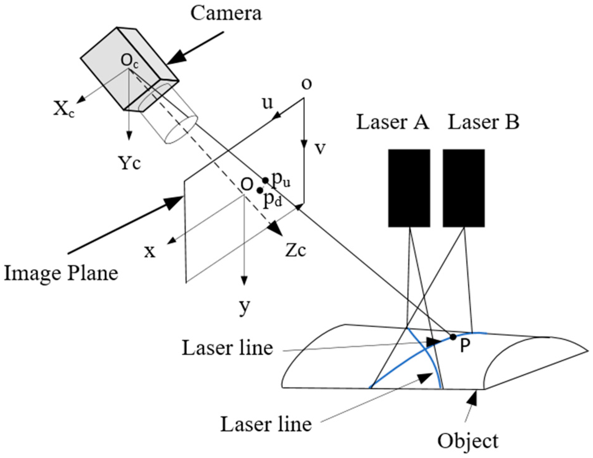
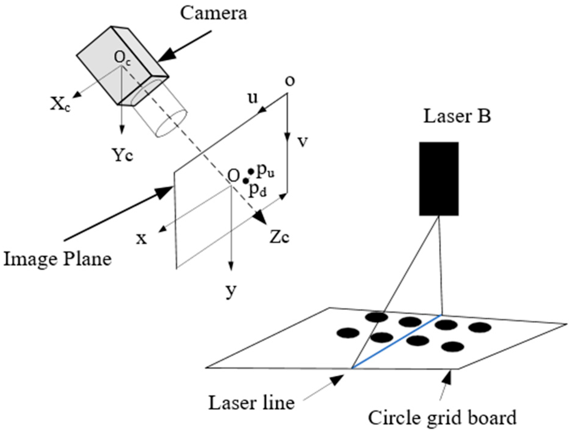
2.1. Model
2.2. 3D Reconstruction
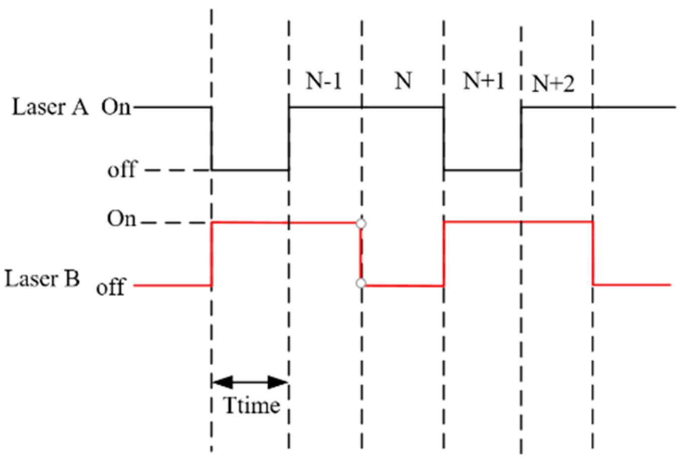
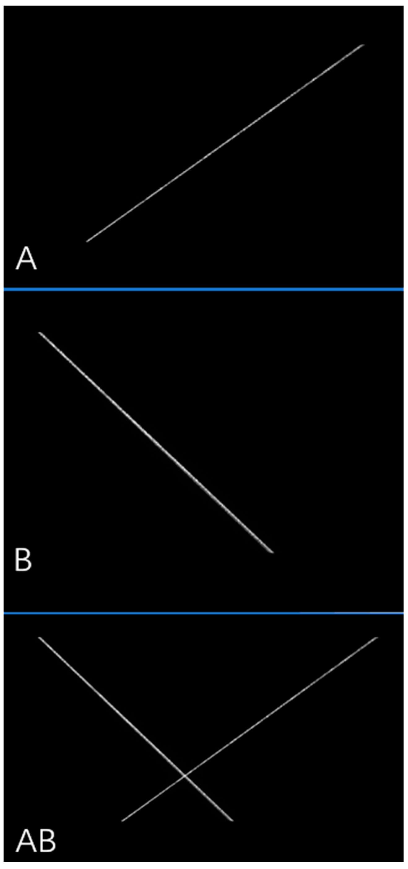
2.3. Laser Line Extraction
2.4. Hand–Eye Calibration
2.5. Laser Plane Extraction
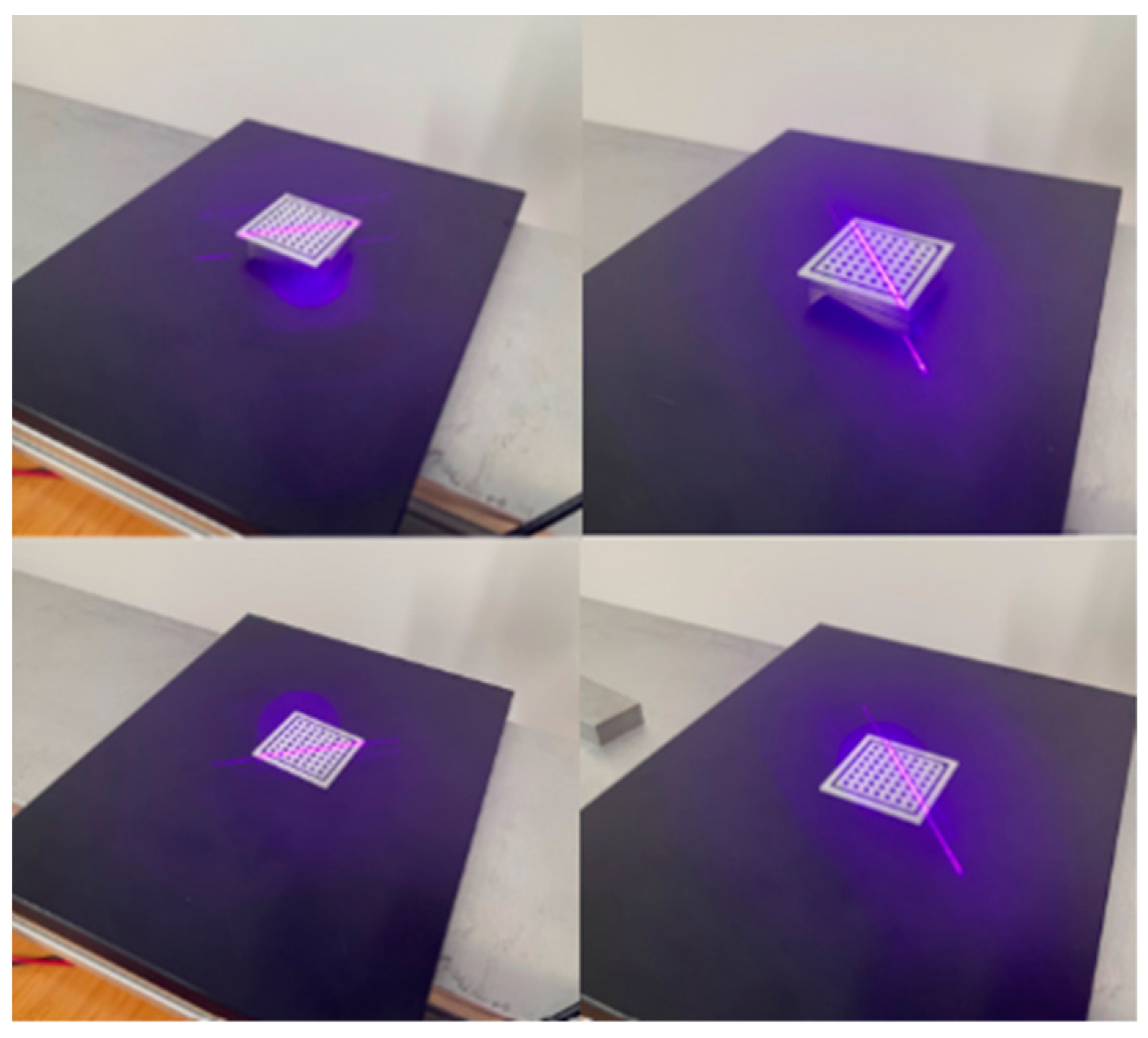
3. Experiment
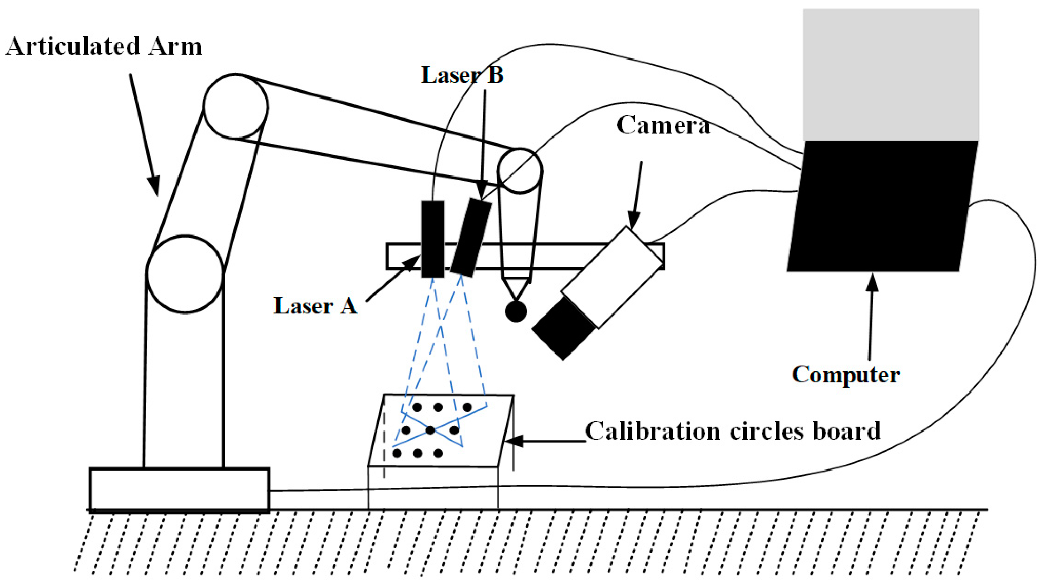
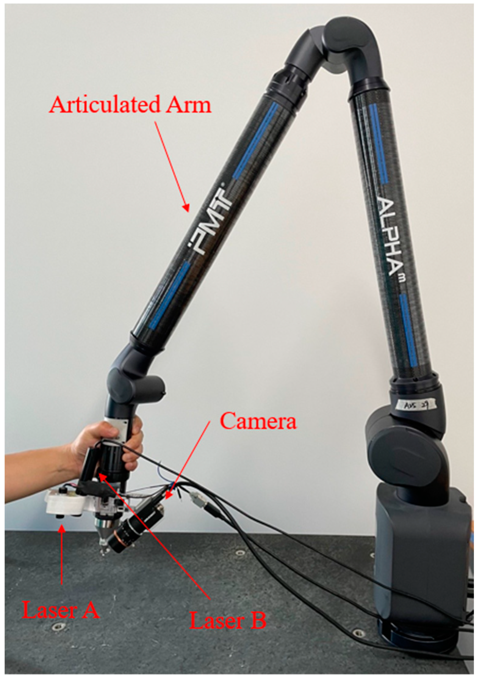
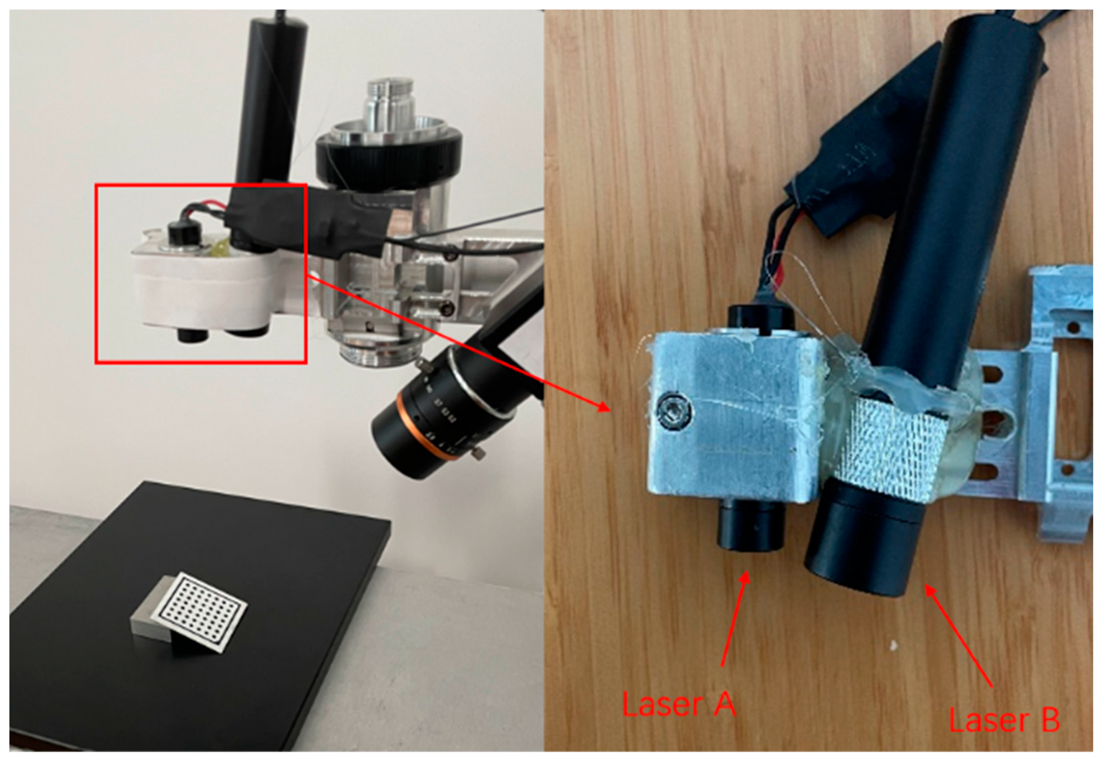
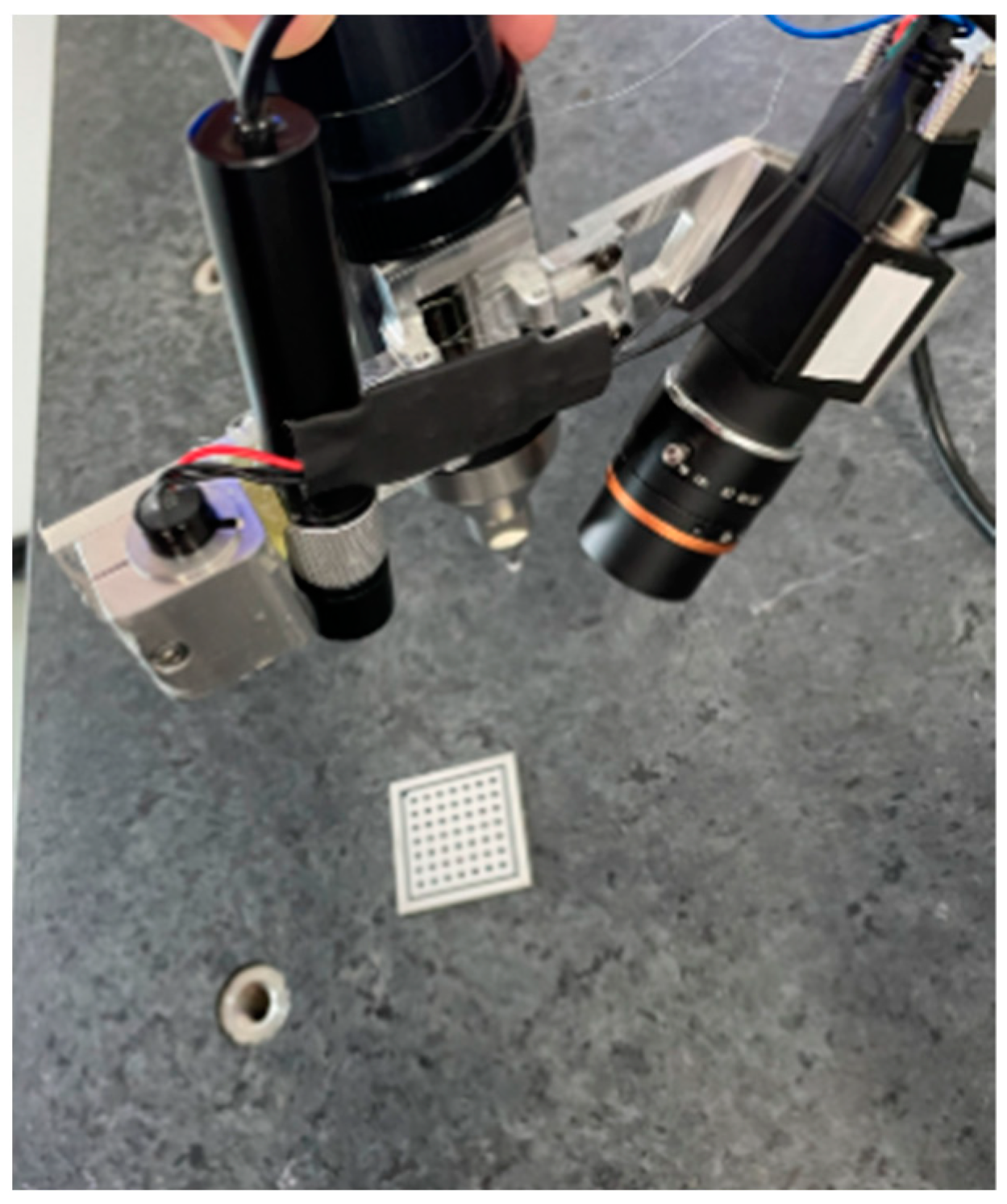
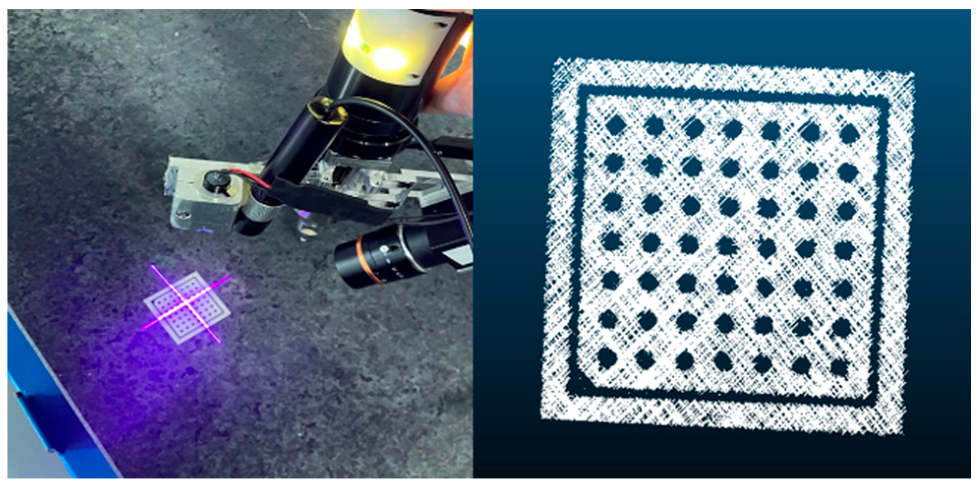
3.1. The Hardware System
- (1)
- Precision of the measuring arm: 0.02 mm
- (2)
- For the 2D camera:
- (a)
- Field of view: 62–72 mm
- (b)
- Acquisition rate: 80 frames per second (FPS)
- (c)
- Resolution: 3072 × 2048 pixels
- (d)
- Working resolution: 2658 × 800 pixels
- (3)
- Linear structured light 3D camera based on camera and laser
- (a)
- Z direction resolution: 0.01–0.012 mm
- (b)
- Laser line resolution (near–far): 0.025–0.028 mm
- (c)
- Laser wavelength: 405 nm
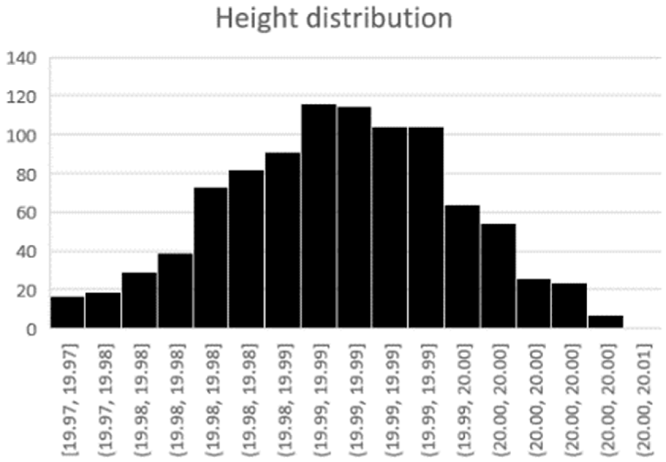
3.2. Calibration of the Camera and Laser Light Plane
3.3. Hand–Eye Calibration
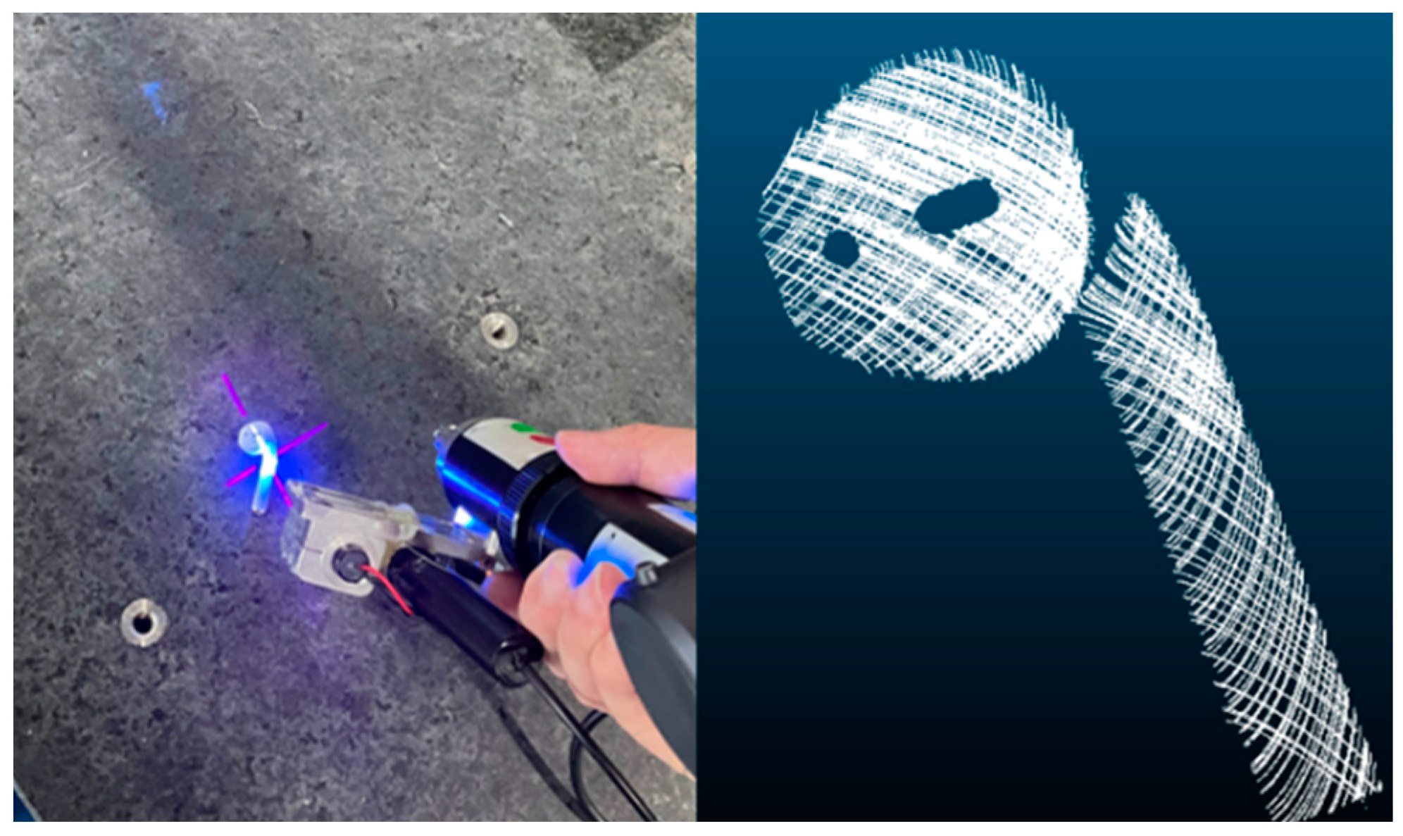
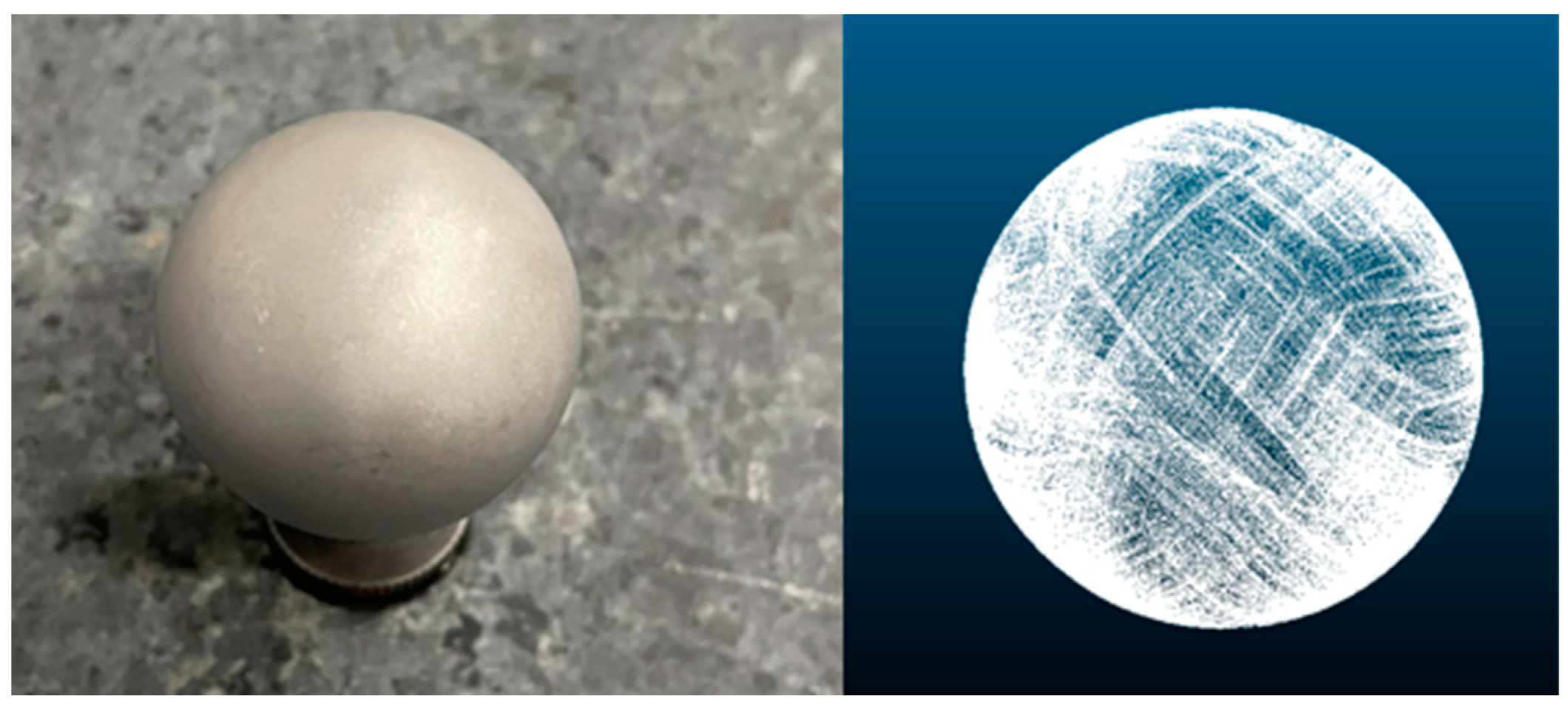
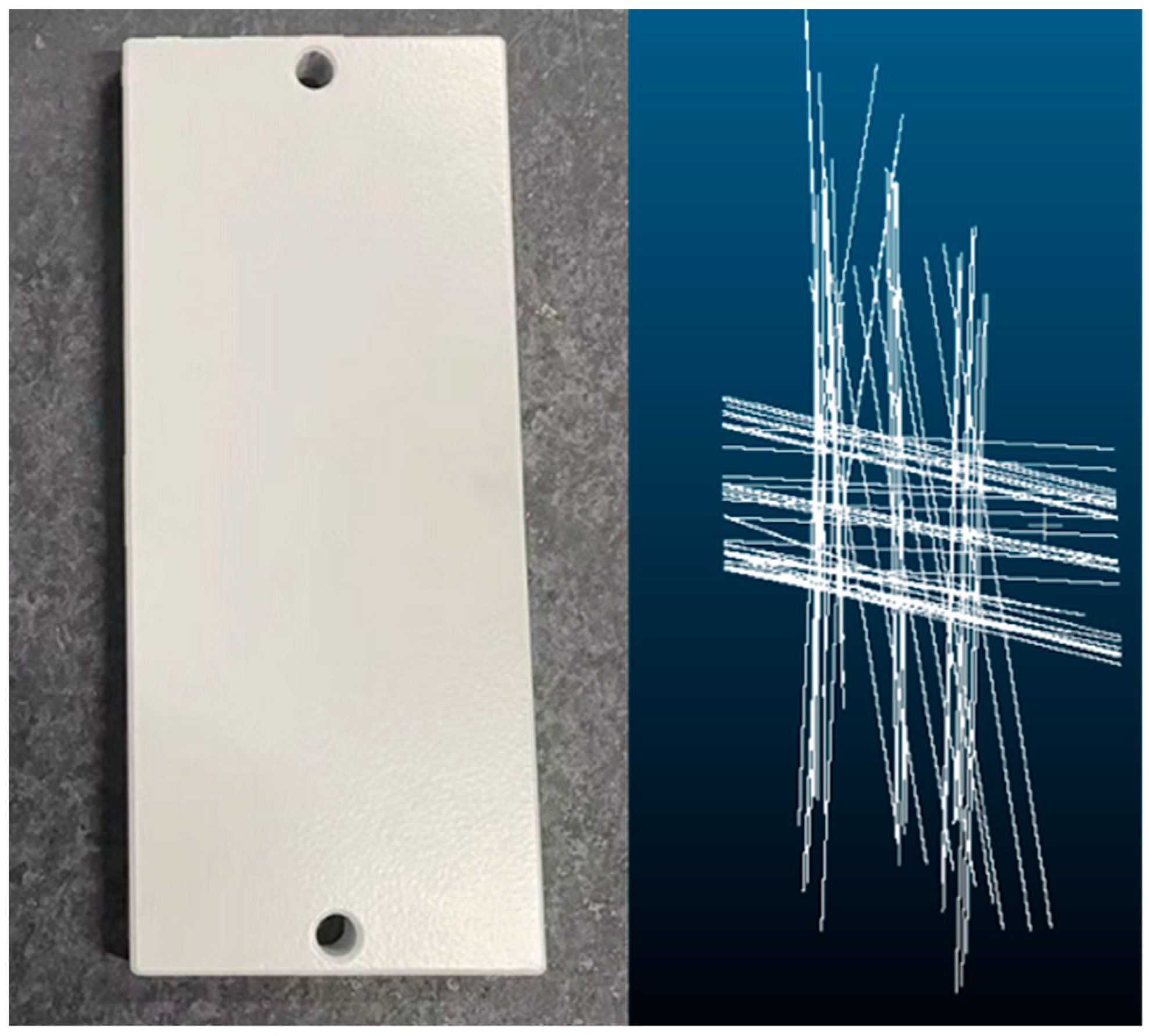
3.4. Scanning Test
4. Conclusions
Author Contributions
Funding
Institutional Review Board Statement
Informed Consent Statement
Data Availability Statement
Conflicts of Interest
References
- Lin, A.C.; Hui-Chin, C. Automatic 3D measuring system for optical scanning of axial fan blades. Int. J. Adv. Manuf. Technol. 2011, 57, 701–717. [Google Scholar] [CrossRef]
- Mei, Q.; Gao, J.; Lin, H.; Chen, Y.; Yunbo, H.; Wang, W.; Zhang, G.; Chen, X. Structure light telecentric stereoscopic vision 3D measurement system based on Scheimpflug condition. Opt. Lasers Eng. 2016, 86, 83–91. [Google Scholar] [CrossRef]
- Choi, K.H.; Song, B.R.; Yoo, B.S.; Choi, B.H.; Park, S.R.; Min, B.H. Laser scan-based system to measure three dimensional conformation and volume of tissue-engineered constructs. Tissue Eng. Regen. Med. 2013, 10, 371–379. [Google Scholar] [CrossRef]
- Huang, K. Research on the Key Technique of Flexible Measuring Arm Coordinate Measuring System; Huazhong University of Science and Technology: Wuhan, China, 2010. [Google Scholar]
- Chen, J.; Wu, X.; Wang, M.Y.; Li, X. 3D shape modeling using a self-developed hand-held 3D laser scanner and an efficient HT-ICP point cloud registration algorithm. Opt. Laser Technol. 2013, 45, 414–423. [Google Scholar] [CrossRef]
- Galantucci, L.M.; Piperi, E.; Lavecchia, F.; Zhavo, A. Semi-automatic low cost 3D laser scanning system for reverse engineering. Procedia CIRP 2015, 28, 94–99. [Google Scholar] [CrossRef]
- Zhang, X.P.; Wang, J.Q.; Zhang, Y.X.; Wang, S.; Xie, F. Large-scale there dimensional stereo vision geometric measurement system. Acta Opt. Sin. 2012, 32, 140–147. [Google Scholar]
- Zhang, L.; Ye, Q.; Yang, W.; Jiao, J. Weld line detection and tracking via spatial-temporal cascaded hidden Markov models and cross structured light. IEEE Trans. Instrum. Meas. 2014, 63, 742–753. [Google Scholar] [CrossRef]
- Yu, Z.J.; Wang, W.; Wang, S.; Chang, Z.J. An online matchin method for binocular vision measurement by using cross lin structured light. Semicond. Optoelectron. 2017, 38, 445–458. [Google Scholar]
- Bleier, M.; Nüchter, A. Low cost 3D laser scanning in air or water using self-calibrating structured light. Int. Arch. Photogramm. Remote Sens. Spat. Inf. Sci. 2017, 42, 105. [Google Scholar] [CrossRef]
- Liu, S.; Tan, Q.; Zhang, Y. Shaft diameter measurement of using the line structured light vision. Sensors 2015, 15, 19750–19767. [Google Scholar] [CrossRef] [PubMed]
- Zhang, Z. A flexible new technique for camera calibration. IEEE Trans. Pattern Anal. Mach. Intell. 2000, 22, 1330–1334. [Google Scholar] [CrossRef]
- Chou, J.C.; Kamel, M. Finding the Position and Orientation of a Sensor on a Robot Manipulator Using Quaternions. Int. J. Robot. Res. 1991, 10, 240–254. [Google Scholar] [CrossRef]


Disclaimer/Publisher’s Note: The statements, opinions and data contained in all publications are solely those of the individual author(s) and contributor(s) and not of MDPI and/or the editor(s). MDPI and/or the editor(s) disclaim responsibility for any injury to people or property resulting from any ideas, methods, instructions or products referred to in the content. |
© 2023 by the authors. Licensee MDPI, Basel, Switzerland. This article is an open access article distributed under the terms and conditions of the Creative Commons Attribution (CC BY) license (https://creativecommons.org/licenses/by/4.0/).
Share and Cite
Tai, D.; Wu, Z.; Yang, Y.; Lu, C. A Cross-Line Structured Light Scanning System Based on a Measuring Arm. Instruments 2023, 7, 5. https://doi.org/10.3390/instruments7010005
Tai D, Wu Z, Yang Y, Lu C. A Cross-Line Structured Light Scanning System Based on a Measuring Arm. Instruments. 2023; 7(1):5. https://doi.org/10.3390/instruments7010005
Chicago/Turabian StyleTai, Dayong, Zhixiong Wu, Ying Yang, and Cunwei Lu. 2023. "A Cross-Line Structured Light Scanning System Based on a Measuring Arm" Instruments 7, no. 1: 5. https://doi.org/10.3390/instruments7010005
APA StyleTai, D., Wu, Z., Yang, Y., & Lu, C. (2023). A Cross-Line Structured Light Scanning System Based on a Measuring Arm. Instruments, 7(1), 5. https://doi.org/10.3390/instruments7010005