Using Artificial Intelligence in the Reconstruction of Signals from the PADME Electromagnetic Calorimeter

Abstract

The PADME apparatus was built at the Frascati National Laboratory of INFN to search for a dark photon ($A^{\prime }$) produced via the process $e^{+}{e}^{-}\to A^{\prime }\gamma$. The central component of the PADME detector is an electromagnetic calorimeter composed of 616 BGO crystals dedicated to the measurement of the energy and position of the final state photons. The high beam particle multiplicity over a short bunch duration requires reliable identification and measurement of overlapping signals. A regression machine-learning-based algorithm has been developed to disentangle with high efficiency close-in-time events and precisely reconstruct the amplitude of the hits and the time with sub-nanosecond resolution. The performance of the algorithm and the sequence of improvements leading to the achieved results are presented and discussed.

1. Introduction

In recent years, the search for an explanation of the Dark Matter phenomenon has led to the development of various hypotheses for an extension of the Standard Model, e.g., Weakly Interacting Massive Particles (WIMPs) [1]. However, the non-observation of new states with mass in the order of 100 GeV led scientists to explore other Dark Matter explanations. The main goal of PADME (Positron Annihilation into Dark Matter Experiment) [2] is to search for the dark photon $A^{\prime }$, a hypothetical gauge boson connecting the dark and the visible sector. In the case of non-vanishing interaction strength ${\alpha }^{\prime }$ with the electrons, $A^{\prime }$ can be produced in the annihilation process of beam positrons with electrons from the target:

$$e^{+}{e}^{-}\to A^{\prime }\gamma .$$

(1)

Knowing the four-momenta of the beam’s positrons, the electrons at rest and the photon produced in the process, the missing mass of the dark photon can be calculated:

$$M_{miss}^2={(P_{e^{+}}+P_{e^{-}}-P_{\gamma })}^2.$$

(2)

The positron beam provided by the DAΦNE LINAC [3] can reach energies up to 550 MeV, providing a limit for the missing mass of 23.7 MeV, and is composed of bunches with a 50 Hz rate. Each bunch contains about $2\times {10}^4$ particles and its length can be varied with typical values of 200–300 ns.

The two main processes contributing to the background, are the annihilation $e^{+}{e}^{-}\to \gamma \gamma \left(\gamma \right)$ and Bremsstrahlung events $e^{+}N\to e^{+}N\gamma$.

To suppress the background from $e^{+}{e}^{-}\to \gamma \gamma \left(\gamma \right)$, the PADME experiment should have high photon detection efficiency, while for the rejection of $e^{+}N\to e^{+}N\gamma$, the radiating positron should be detected and a reliable matching in time between the positron and the emitted photon should be assured.

The initial studies based on a full Geant4 [4] simulation indicate that the PADME experiment can reach sensitivies in ${\alpha }^{\prime }$ down to ${10}^{-8}$ [5] with high-efficiency detectors (greater than 99%) and time resolution better than 1 ns. In addition, due to the high bunch multiplicity, double-pulse separation capabilities are required for each of the chosen detectors.

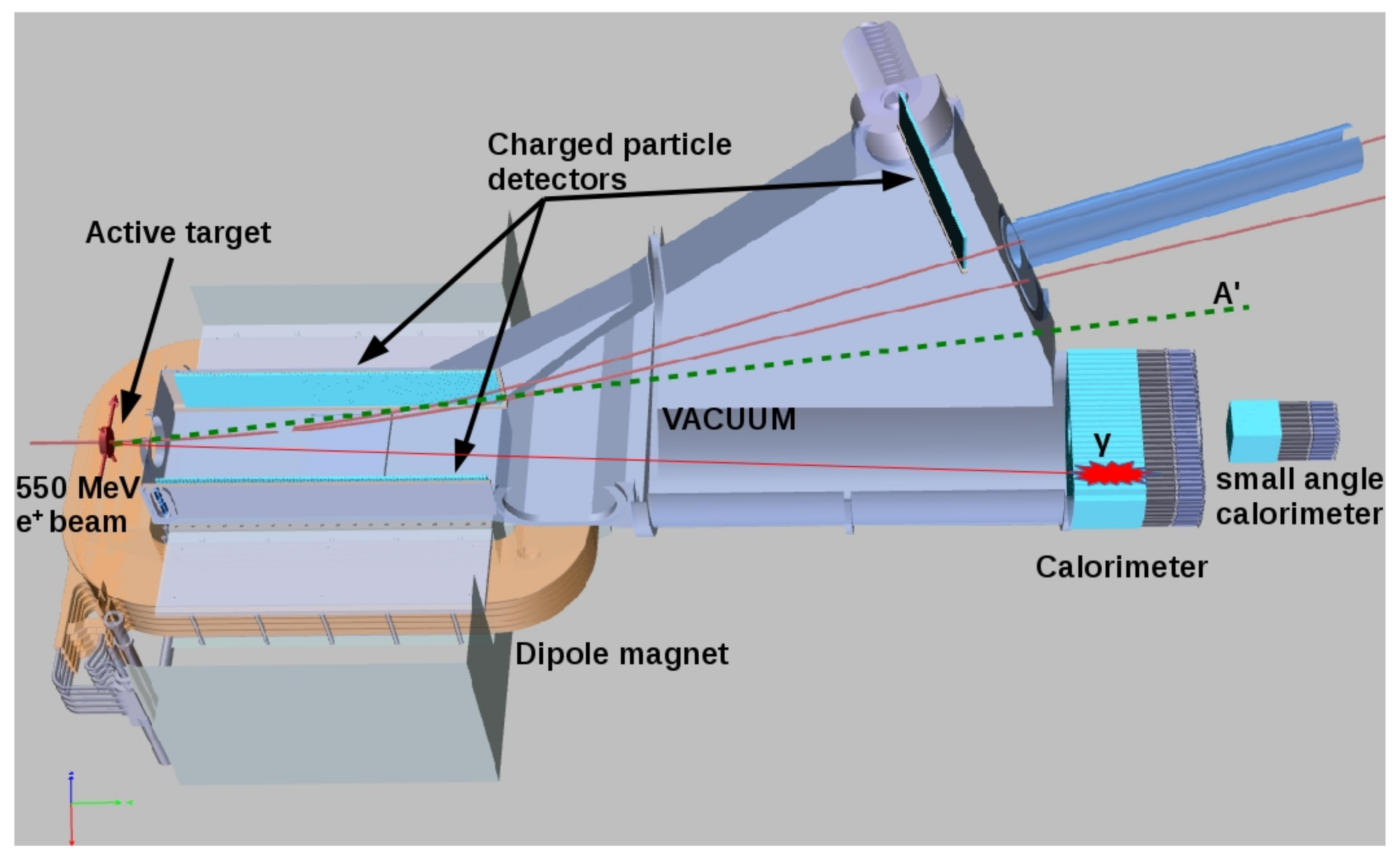
2. The Padme Experiment

A sketch of the PADME experiment is shown in Figure 1. A short description of its major detector components [6] follows.

2.1. Active Target

The target [7] is composed of polycrystalline diamond (Z = 6) since low Z is required to increase the annihilation to bremsstrahlung cross-section ratio. The target has a 100 $\mathsf{\mu }$m thickness and 20 mm width and length. Apart from providing the target for the annihilation process, it also measures the beam’s multiplicity and XY profile. For this reason 16 horizontal and 16 vertical graphite electrodes of 1 mm width are engraved onto the target using an excimer laser.

2.2. Charged Particle Detectors

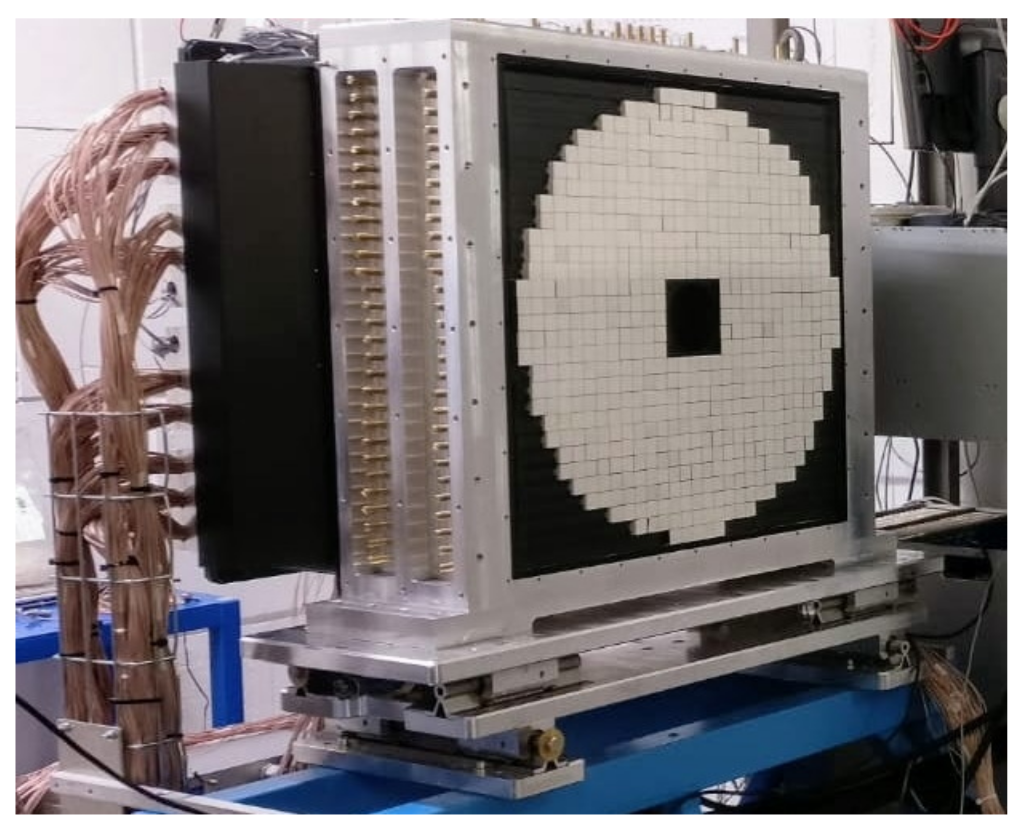
Three sets of detectors register the charged particles. The beam positrons may lose energy in the target and produce Bremsstrahlung photons, detected by the electromagnetic calorimeter, which need to be rejected. This is achieved by coinciding these photons with the particles that produced them. These particles are detected by the positron and high energy positron vetoes. In case the $A^{\prime }$ decays into an $e^{+}{e}^{-}$ pair, the electron will be registered by the electron veto. All three charged particle detectors are composed of $10\times 10\times 178$ mm${}^3$ plastic scintillators with WLS fibers coupled to $3\times 3$ mm${}^2$ Hamamatsu S13360 silicon photomultipliers with 25 $\mathsf{\mu }$m pixel size and are placed in ${10}^{-5}$ mbar vacuum. The positron and the electron vetoes are located inside the magnet and are composed of 90 and 96 scintillating bars, respectively. Both detect particles with momenta between 50 and 450 MeV. The high energy positron veto is located next to the beam exit window and is composed of 16 scintillating bars, with scintillation light read out on both sides. It allows the detection of positrons with momenta between 450 and 500 MeV.

The charged particle detectors segmentation provides measurement of the $e^{+}/e^{-}$ momentum with a resolution of $\approx$5%. The time resolution is 700 ps [8].

2.3. Calorimeters

The PADME calorimetric system is composed of an Electromagnetic Calorimeter (ECal) and a small-angle calorimeter (SAC). The ECal (Figure 2) is composed of 616 BGO cystals measuring $2.1\times 2.1\times 23$ cm${}^3$, connected to HZC 1912 photomultipliers. The optical isolation of the crystals is achieved by covering them with diffuse reflective TiO${}_2$ paint and additionally with 50–100 $\mathsf{\mu }$m thin black Tedlar foils. The ECal is placed 3.45 m away from the target and has a radius of 29 cm, thus achieving an angular coverage between 15 and 84 mrad. The lower limit is due to a square hole in its center, which is covered by the SAC. The scintillation light decay time is 300 ns. Calibration was performed both with a ${}^{22}$Na source before constructing the calorimeter and then subsequently with cosmic rays. The energy resolution is ∼7% at $E_{\gamma }=100$ MeV [9].

The Small Angle Calorimeter (SAC) [10] is located downstream of the ECal and mainly detects photons produced by Bremsstrahlung events. To suppress this type of background, the data from the SAC is matched in time with the data from the charged particle detectors. In addition, the SAC detects photons from multiphoton annihilation events. The SAC is composed of 25 PbF${}_2$ crystals measuring $3\times 3\times 14$ cm${}^3$ and covers an angle between 0 and 15 mrad.

2.4. Readout System

The PADME Data Acquisition System consists of 29 CAEN V1742 ADC boards, each equipped with 32 analog and 2 trigger input channels. The V1742 switch capacitor digitizer employs the DRS4 chip, capable of sampling the input signal at 750 MS/s, 1 GS/s, 2.5 GS/s, and 5 GS/s. Complete waveforms of 1024 samples for each channel are recorded upon a beam-based trigger signal. In the case of the electromagnetic calorimeter which is sampled at 1 GS/s, this corresponds to a $\approx$1 $\mathsf{\mu }$s recorded waveform.

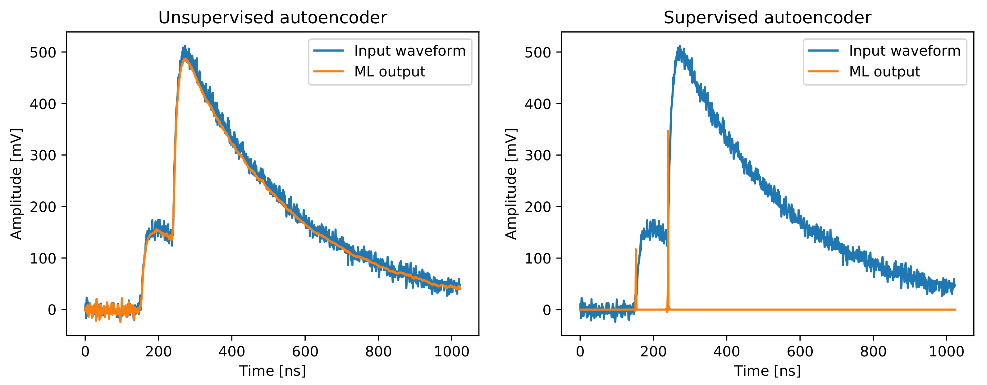
3. Application of Neural Networks for Waveform Description

The high multiplicity of the positron beam in combination with the short bunch duration leads to many overlapping or close-in-time signals recorded in a single event. One way to solve this problem is to use neural networks (NNs) to count the signals from the electromagnetic calorimeter in each event, to identify and separate overlapping signals, and to extract signal parameters—the arrival times of the individual signals and their amplitudes. To train the NNs, an event simulation was developed. Each event represents a waveform of 1024 samples, for which the number of signals as well as the individual signal parameters can be varied. Various sets of waveforms $A\left(t\right)$ were generated, containing a random number of signals with shapes defined by the subtraction of two exponents

$$A\left(t\right)=A_0(e^{-(t-t_0)/{\tau }_1}-e^{-(t-t_0)/{\tau }_2}),t\ge t_0,$$

(3)

where $t_0$ is the arrival time of the signal, ${\tau }_1$ is the signal decay time, taken to be 300 ns, and ${\tau }_2$ is related to the signal rise time, taken to be 10 ns. These values are typical for the PADME PMT + BGO crystal assembly. $A_0$ is the signal amplitude parameter, chosen to follow a Gaussian distribution. The arrival time follows a uniform distribution with a minimum value of $t_0=100$ ns, to account for the trigger specifications. For the training of the networks presented here, a mean value $A_0=200$ mV with $\sigma =200$ mV was used and an additional lower limit $A_0>20$ mV was set. The signals from the ECal are digitised by an ADC with 1 V dynamic range, which should be sufficient for the maximal energy cell within an electromagnetic shower. Since the selected photon energy is between 50 MeV and 450 MeV, a 200 mV mean amplitude was chosen to increase the training statistics to signals corresponding to the 100 MeV range. All waveforms include a Gaussian noise with a mean value of 10 mV added in each bin. A predefined maximum number of four signals was used for all generated waveforms. Many of the events, recorded by the ECal contain only one or two signals, however, there are events with more recorded signals which requires the inclusion of such cases in the training. Different NNs were trained on the thus generated events and each network is trained on 100,000 events.

For the implementation of all neural networks presented in this study and for the output analysis were used the ROOT [11], TensorFlow [12] and Keras [13] frameworks. Three different convolutional neural networks (CNNs) [14] were developed, starting with the classification task of dividing the events into categories based on the number of signals in them and moving to regression tasks with the aim of signal parameter estimation.

The first CNN performs a classification task aimed at counting the number of signals in each waveform. It consists of a single convolutional layer, followed by three fully connected layers. This network was trained using labels containing only information about the number of signals in each event. The obtained model was then applied for the simulated set of events with two generated signals and the output was compared to the true labels. Figure 3 shows the efficiency of the signal counting as a function of $\Delta t=|t_2-t_1|$ where $t_2$ and $t_1$ are the arrival times of the two signals. The efficiency is 50% for $\Delta t=10$ ns and 100% for $\Delta t>50$ ns.

The estimation of signal parameters requires the development of networks with more complex architectures. Convolutional autoencoders [15] can be used for extracting useful data from waveforms.

An autoencoder was developed with the targeted output replicating the original waveform. The neural network architecture consists of three convolutional layers followed by three deconvolutional layers with the same parameters and a single final deconvolutional layer for setting the output dimensions. Figure 4 (left) shows an example of the original and the output waveform for an event with two signals. It is observed that such networks can reproduce the signals, which represents the main motivation for applying this architecture for signal parameter estimation through supervised learning.

A modified autoencoder trained on labeled data was developed with training based on output arrays of the same length as the input waveforms. On the positions of signal arrival, the value is set to the signal amplitude and all other values are set to 0. An example of the output of the modified autoencoder and its corresponding waveform is presented in Figure 4 (right).

To assess the modified autoencoder output and compare it with the original data labels, a reconstruction algorithm was developed. The data labels contain an array of 1024 numbers with a single non-zero amplitude value at the arrival time $t_0$ for each generated signal. The NN output gives multiple amplitude values over a number of time positions for each recognised signal, usually with a maximum on the most probable position and decreasing values on both of its sides. The reconstruction algorithm locates the maximum and adds the values of the three positions before it and the three positions after it to the maximum value. The result is taken to be the amplitude of the reconstructed signal and the time position of the maximum is taken to be the arrival time of this signal. The reconstruction is also applied to the original data labels and the results for the reconstructed output are then compared to them. This allows both for comparison of the amplitude value of the original and reconstructed signal, as well as evaluation of the arrival time and analysis of the neural network efficiency.

4. Signal Parameter Reconstruction

The probability for a signal to be discriminated and the accuracy of the reconstructed signal parameters were studied. The modified autoencoder model was trained on a set of 100,000 events with up to four signals each and was applied to a statistically independent test set, again with 100,000 events containing up to four signals.

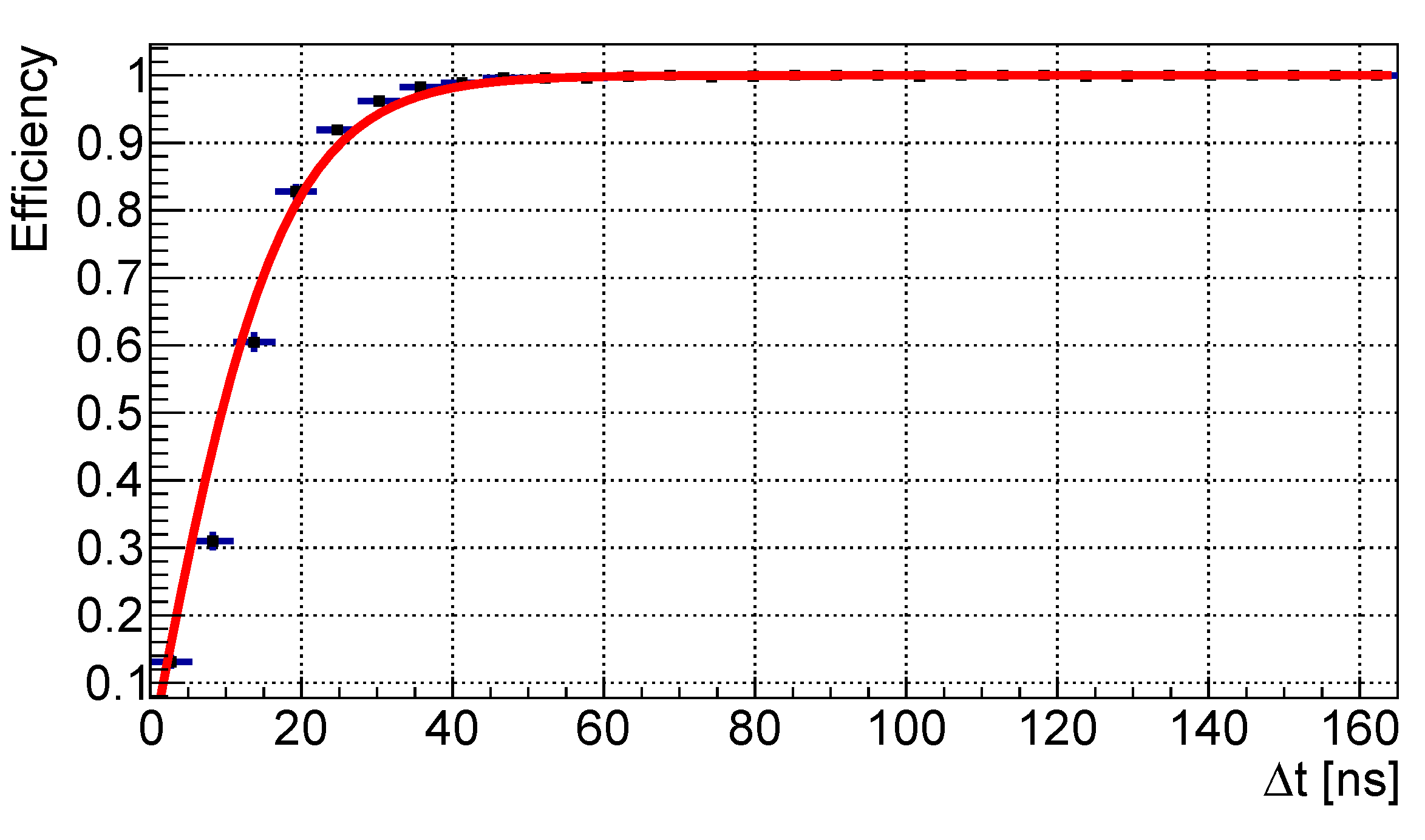
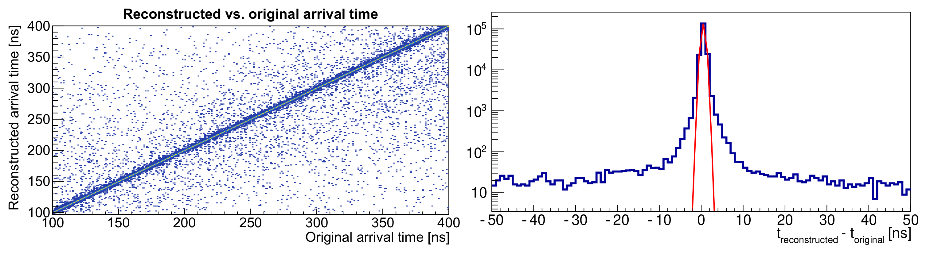
4.1. Time Reconstruction

To study the double-pulse separation abilities of the machine learning algorithm, each simulated signal is associated with the closest-in-time one from the NN output. The left panel in Figure 5 represents the difference between the reconstructed and the original time of the signal arrival. The distribution of this difference (Figure 5, right panel) is symmetric, with $\sigma$∼ 520 ps and RMS ∼ 3.2 ns if assumed Gaussian, however, non-Gaussian tails do exist.

A signal is considered successfully identified if the difference between the original and reconstructed output is less than 2 ns.

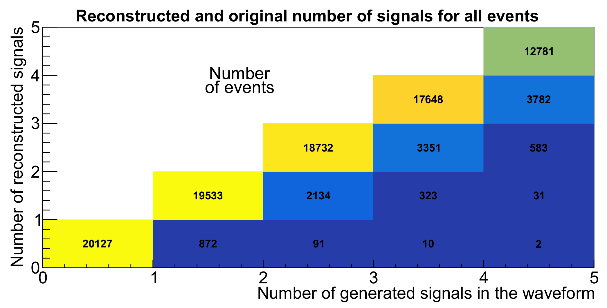
4.2. Signal Recognition

Figure 6 shows all of the events in the test set, divided into bins based on the number of reconstructed signals and the originally generated ones. Ideally, these two numbers should be the same for all events. However, two major factors influence signal discrimination: a small difference in signal arrival time may cause two or more signals to be merged into one and signals with small amplitudes may not be identified above the noise.

Signals with time differences less than 10 ns are merged into a single hit and most events with amplitudes smaller than 50 mV are not likely to be identified, which results in decreased efficiency, as seen in Figure 7.

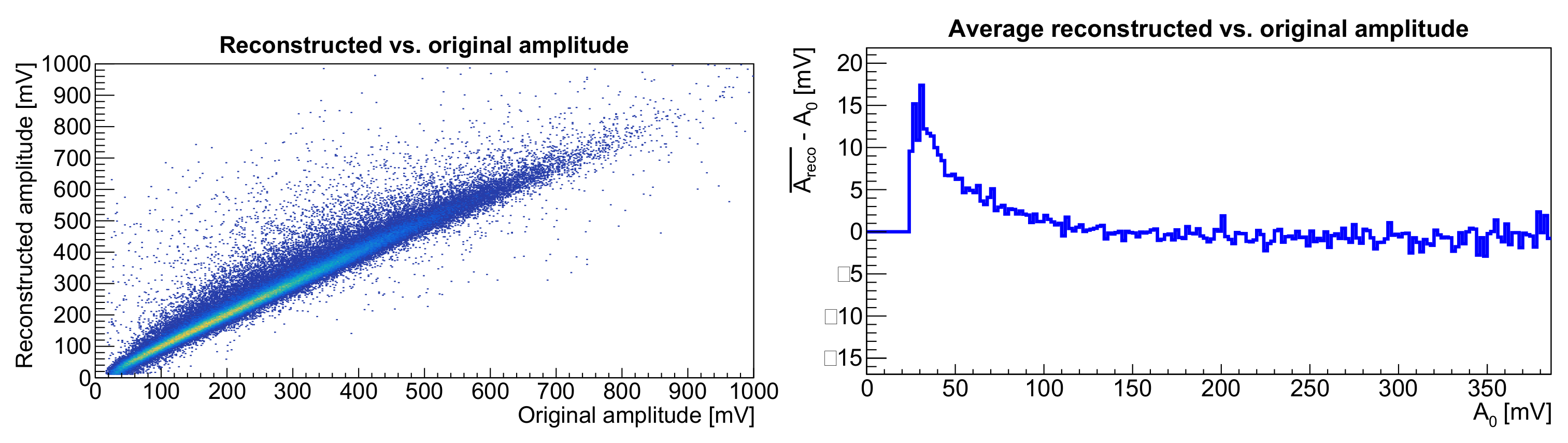
4.3. Amplitude Reconstruction

The developed CNN provides reconstruction of the signal amplitude values. The reconstructed versus the original amplitudes for the successfully identified signals are shown in the left panel of Figure 8. The correlation is well pronounced. To quantitatively compare the quality of signal identification, the average difference between the reconstructed and the true amplitude value for each 2 mV interval of generated amplitude is shown in the right panel of Figure 8.

The inaccuracy of the small amplitude values can be compensated for by a dedicated calibration of the NN output.

5. Conclusions

The high particle rate in the PADME calorimeter requires implementation of advanced reconstruction algorithms to achieve less than 1 ns time resolution of the reconstructed showers. Machine learning methods were applied for the successful identification of calorimeter signals and for the extraction of signal parameters. A CNN with a single convolutional layer was used to count the number of signals in an event. A modified CNN autoencoder was probed for the estimation of signal parameters—arrival time and amplitude. The performance of the networks was assessed through a specially designed algorithm, comparing the network output with the original data labels. The CNN provides time reconstruction with ∼500 ps time resolution and the amplitude is reconstructed in the 30–700 mV range. There is an inaccuracy for amplitudes less than 100 mV, which can be solved by an additional calibration of the NN output or by developing networks with modified architectures specifically targeting small amplitudes.

References

1. Alexander, J.; Battaglieri, M.; Echenard, B.; Essig, R.; Graham, M.; Izaguirre, E.; Jaros, J.; Krnjaic, G.; Mardon, J.; Morrissey, D.; et al. Dark Sectors 2016 Workshop: Community Report. arXiv 2016, arXiv:hep-ph/1608.08632. [Google Scholar]
2. Raggi, M.; Kozhuharov, V. Proposal to Search for a Dark Photon in Positron on Target Collisions at DAΦNE Linac. Adv. High Energy Phys. 2014, 2014, 959802. [Google Scholar] [CrossRef]
3. Valente, P.; Belli, M.; Bolli, B.; Buonomo, B.; Cantarella, S.; Ceccarelli, R.; Cecchinelli, A.; Cerafogli, O.; Clementi, R.; Di Giulio, C.; et al. Linear Accelerator Test Facility at LNF Conceptual Design Report. arXiv 2016, arXiv:physics.acc-ph/1603.05651. [Google Scholar]
4. Agostinelli, S.; Allison, J.; Amako, K.A.; Apostolakis, J.; Araujo, H.; Arce, P.; Asai, M.; Axen, D.; Banerjee, S.; Barrand, G.J.N.I.; et al. GEANT4—A simulation toolkit. Nucl. Instrum. Methods Phys. Res. Sect. A Accel. Spectrometers Detect. Assoc. Equip. 2003, 506, 250–303. [Google Scholar] [CrossRef]
5. Raggi, M.; Kozhuharov, V.; Valente, P. The PADME experiment at LNF. EPJ Web Conf. 2015, 96, 01025. [Google Scholar] [CrossRef]
6. Albicocco, P.; Assiro, R.; Bossi, F.; Branchini, P.; Buonomo, B.; Capirossi, V.; Capitolo, E.; Capoccia, C.; Caricato, A.P.; Ceravolo, S.; et al. Commissioning of the PADME experiment with a positron beam. arXiv 2022, arXiv:physics.ins-det/2205.03430. [Google Scholar] [CrossRef]
7. Assiro, R.; Caricato, A.P.; Chiodini, G.; Corrado, M.; De Feudis, M.; Di Giulio, C.; Fiore, G.; Foggetta, L.; Leonardi, E.; Martino, M.; et al. Performance of the diamond active target prototype for the PADME experiment at the DAPHNE BTF. Nucl. Instrum. Methods Phys. Res. Sect. A Accel. Spectrometers Detect. Assoc. Equip. 2018, A898, 105–110. [Google Scholar] [CrossRef]
8. Ferrarotto, F.; Foggetta, L.; Georgiev, G.; Gianotti, P.; Kozhuharov, V.; Leonardi, E.; Piperno, G.; Raggi, M.; Taruggi, C.; Tsankov, L.; et al. Performance of the Prototype of the Charged-Particle Veto System of the PADME Experiment. IEEE Trans. Nucl. Sci. 2018, 65, 2029–2035. [Google Scholar] [CrossRef]
9. Albicocco, P.; Alexander, J.; Bossi, F.; Branchini, P.; Buonomo, B.; Capoccia, C.; Capitolo, E.; Chiodini, G.; Caricato, A.P.; de Sangro, R.; et al. Characterisation and performance of the PADME electromagnetic calorimeter. J. Instrum. 2020, 15, T10003. [Google Scholar] [CrossRef]
10. Frankenthal, A.; Alexander, J.; Buonomo, B.; Capitolo, E.; Capoccia, C.; Cesarotti, C.; De Sangro, R.; Di Giulio, C.; Ferrarotto, F.; Foggetta, L.; et al. Characterization and performance of PADME’s Cherenkov-based small-angle calorimeter. Nucl. Instrum. Methods Phys. Res. Sect. A Accel. Spectrometers Detect. Assoc. Equip. 2019, 919, 89–97. [Google Scholar] [CrossRef]
11. Brun, R.; Rademakers, F. ROOT: An object oriented data analysis framework. Nucl. Instrum. Methods Phys. Res. Sect. A Accel. Spectrometers Detect. Assoc. Equip. 1997, 389, 81–86. [Google Scholar] [CrossRef]
12. Abadi, M.; Agarwal, A.; Barham, P.; Brevdo, E.; Chen, Z.; Citro, C.; Corrado, G.S.; Davis, A.; Dean, J.; Devin, M.; et al. TensorFlow: Large-Scale Machine Learning on Heterogeneous Systems. 2015. Available online: https://tensorflow.org (accessed on 11 July 2022).
13. Chollet, F. Keras. 2015. Available online: https://keras.io (accessed on 11 July 2022).
14. O’Shea, K.; Nash, R. An Introduction to Convolutional Neural Networks. arXiv 2015, arXiv:cs.NE/1511.08458. [Google Scholar]
15. Zhang, Y. A better autoencoder for image: Convolutional autoencoder. In Proceedings of the ICONIP17-DCEC, Guangzhou, China, 14–18 October 2017; Available online: http://users.cecs.anu.edu.au/~Tom.Gedeon/conf/ABCs2018/paper/ABCs2018_paper_58.pdf (accessed on 11 July 2022).
Figure 1. Outline of the PADME experiment.
Instruments 06 00046 g001
Figure 2. The PADME Electromagnetic Calorimeter.
Instruments 06 00046 g002
Figure 3. Efficiency of a signal-counting CNN as a function of the time difference between two signals. A sigmoid curve for the efficiency Eff = 2 · ( 1 ( 1 + e x p ( Δ t / 70 ) 0.5 ) is fitted (red). For signals with Δ t = 10 ns, the efficiency is 50%. The efficiency reaches 100% for Δ t > 50 ns.
Instruments 06 00046 g003
Figure 4. Autoencoder NN output and the original event with two signals. (Left) classical autoencoder. (Right) modified autoencoder.
Instruments 06 00046 g004
Figure 5. (Left) Reconstructed vs. original time of arrival for all events in the test set. (Right) Distribution of the signals according to the difference between the reconstructed and the original signal arrival time. The red curve represents a Gaussian distribution with σ 520 ps and mean value of 0.
Instruments 06 00046 g005
Figure 6. Number of reconstructed signals versus the original number of generated signals in the test sample.
Instruments 06 00046 g006
Figure 7. (Left) Matched (blue) and missed (red) events as a function of the arrival time difference Δ t for events with two generated signals. (Right) Matched (blue) and missed (red) events as a function of the amplitude value for events with one generated signal. Missed events with high time differences are due to small amplitudes.
Instruments 06 00046 g007
Figure 8. (Left) All events based on their reconstructed amplitude value and the original one (Right) Difference between the average value of the reconstructed amplitude A r e c o ¯ and the original value A 0 for each original value A 0 , divided into 2 mV bins. It can be observed that for small amplitudes the reconstructed value is higher than the original one.
Instruments 06 00046 g008
Publisher’s Note: MDPI stays neutral with regard to jurisdictional claims in published maps and institutional affiliations.