1. Introduction
Various types of magnets play important roles in many physics laboratories. Unfortunately, they are often expensive and require long lead times to order. Here we propose a complementary method: we constructed multipole magnets from standard-size permanent-magnet cubes, which are reasonably inexpensive and easy to obtain. Moreover, we suggest to hold them in 3D-printed frames or CNC-machined aluminum frames that can be produced in most small workshops. By constructing the frames in two halves, they can be wrapped-around or strapped-on to circular pipes and easily fixed with non-magnetic screws, which makes retrofitting them to existing beam lines very simple.
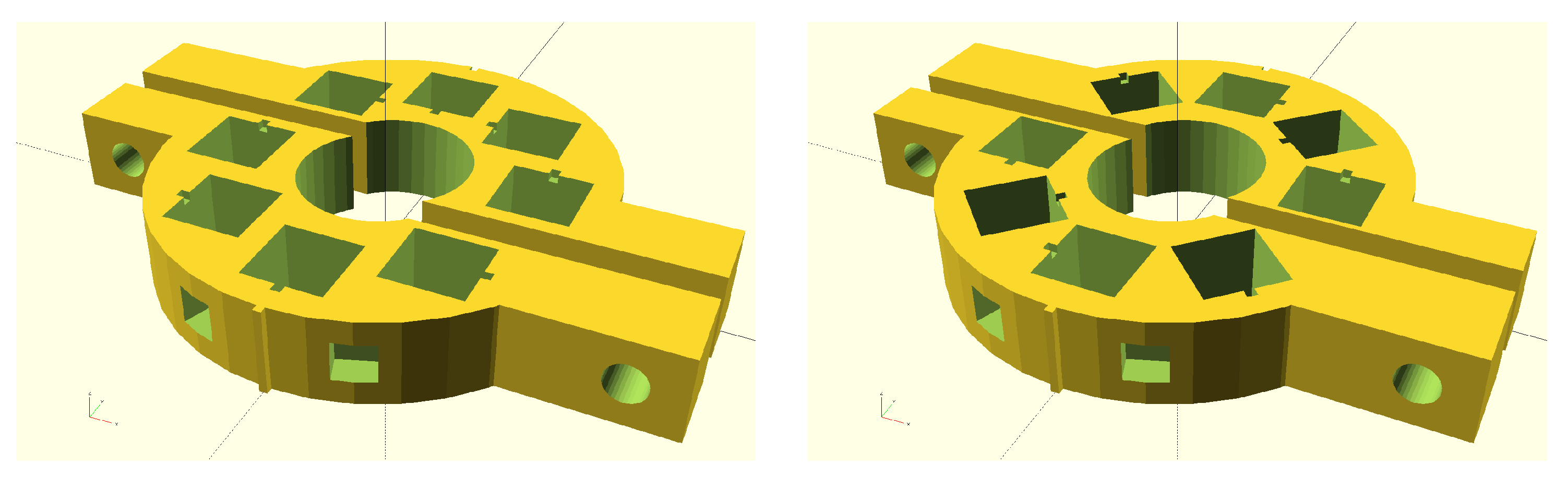
Figure 1 illustrates the frames for a dipole and a quadrupole constructed from eight cubes, each.
The orientation of the cubes in the frames follows the Halbach method [
1], adapted to square [
2] instead of trapezoidal magnet segments. In an
M-magnet dipole, subsequent magnets along the azimuth are rotated by
. The left-hand image in
Figure 1 illustrates this for a dipole made of eight cubes. In the frame for an eight-magnet quadrupole, shown on the right-hand image in
Figure 1, subsequent magnets rotate by
as illustrated by the little notch in each of the eight holes for the cubes.
In order to calculate the magnetic fields from the cubes in three dimensions, we used the closed-form expressions from [
3], which allowed us to prepare MATLAB [
4] scripts to determine the relevant field quantities and the multipole contents of the magnets in parameterized form. This proves very convenient to adapt the design to different sized cubes, different geometries, and other multipolarities.
The organization of this report is as follows: after we discuss the design of the frames with the OpenSCAD [
5] software, we characterize eight-magnet dipoles, quadrupoles, and solenoids made of 10 mm cubes. Then, we combine two dipoles or quadrupoles to produce dipoles and quadrupoles whose field strength can be varied, where we follow an approach that is complementary to those discussed in [
1,
6,
7]. In order to illustrate the use of the variable multipoles, we combined several such magnets to beam-line modules, which was inspired by the early permanent-magnet based anti-proton recycler ring at Fermilab [
8] and, more recently, by CBETA [
9].
2. Frames
We used OpenSCAD to prepare solid models of the frames to hold the permanent-magnet cubes, because this CAD software is easily scriptable, such that parameters for different-sized magnets of multipoles only require changing a few parameters. The frame can then be exported in a format that is compatible with 3D printers or CNC milling machines, which allows for short prototyping cycles.
The frame consists of a cylinder with an outer radius of
mm, a 1 mm notch and a groove on its outer periphery to tell up from down, and 5 mm square holes to later attach handling rods. Furthermore, there are rectangular solids to later hold screws—the horizontal circular holes shown in
Figure 1. Moreover, a circular hole with a radius of
mm was removed from the center. The holes for the 10 mm cubes were then “stamped out” from this base frame. Each of the holes is born at the center, receives the little notch, and is rotated by an angle
, where
m is the multipolarity of the magnets and
is the azimuthal position of the cube in the frame. Then, it is moved outwards by
mm along the
x-axis before being rotated once again by
, which puts the hole in place. We point out that the notches on the holes are only for orientation; in the magnets, we used that direction to indicate the “feather” (and not the “tip”) of the arrows that indicate the easy axis of the magnets. Typically, the square holes for the cubes are 0.1 mm larger than the magnet cubes themselves, which makes inserting the cubes easier. Inside the holes, they are then easily fixated with super-glue.
Note that these frames have semi-circular holes with a diameter of mm in their center. Again, in order to account for finite tolerances of the frame and the pipe, normally the diameter needs to be increased a little, say, by 0.1 mm. This makes it easy to wrap the frames around a circular pipe, align the holes for the screws, and insert the screws and tighten them. This fixes the frame in place. Moving it along the pipe or rotating it only involves loosening the screws, moving the frame with the magnets, and tightening the screws again.
Let us now investigate the properties of the magnetic field generated by cubes in such a frame—first out are dipoles.
3. Dipole
In [
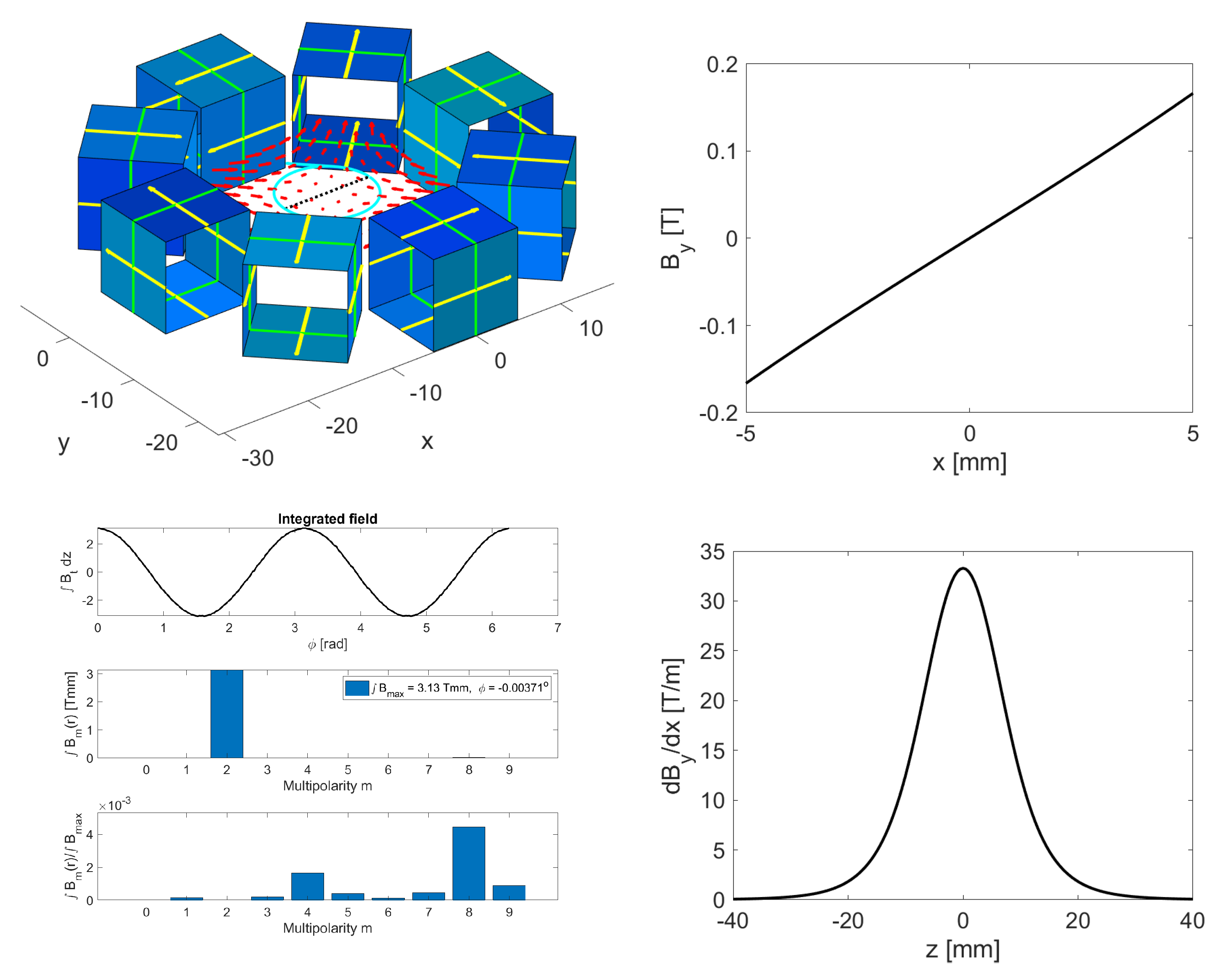
3], we calculated the field generated by a rectangular current sheet, which proved useful to describe permanent-magnet cubes that can be modeled by four rectangular sheets. In the top-left image in
Figure 2, we see that each of the eight magnets consists of four blue sheets with the green line indicating the direction of the current, such that we can visualize the cube as a square solenoid that generates a magnetic field in its inside that is represented by the yellow arrow, which coincides with the direction of the easy axis of the magnet. In all our simulations, we assumed the remanent field of all cubes to be
T. Inside the ring-shaped assembly with the eight cubes, we see red arrows indicating the direction of the field in the mid-plane. The vertical field
along the dotted black line is shown on the top-right plot, which shows a magnitude of about 0.24 T with a curved dependence in the
x-direction, indicating some higher multipole components. The plot on the bottom-right shows
along a line in the
z-direction. We observed that the fringe fields roll off slowly and extend far beyond the
mm physical size of the magnets. Finally, we determined the multipoles of the assembly by integrating the field in the range
mm along lines perpendicular to the cyan circle, which had a radius of 5 mm. We then Fourier-transformed the component of the field that is tangential to this circle and showed it on the upper panel on the bottom-left in
Figure 2. This algorithm, which is explained in [
3], gives us the magnitude and angle of the multipole coefficients of the assembly shown on the middle panel. We see that the integrated field strength was 5.72 Tmm, and the lower panel indicates that the relative magnitude of the other multipoles was around
with the decapole contribution (
) being the largest.
We conclude that the eight-cube dipole magnet reached a peak field of 0.24 T and had an integrated field strength of 5.72 Tmm, while the relative magnitude of unwanted multipoles on a circle with a 5 mm radius was below .
4. Quadrupole
The field of the quadrupole assembly corresponding to the frame from the right in
Figure 1 is shown in
Figure 3. The top-left image shows the eight cubes with the red arrows indicating the field in the mid-plane, the black dotted line, and the cyan circle on which the multipoles were calculated. The top-right plot shows
along the black dotted line and indicates a linearly rising field along the
x-axis that is characteristic for a quadrupole. From the slope, we determined a gradient in the mid-plane of
T/m. The gradient along the
z-axis in the middle of the assembly is visible on the bottom-right plot. We observed that even the fringe fields of the quadrupole extended beyond its physical size of
mm but decayed faster than those of a dipole. The image with the three panels on the bottom-left shows the tangential field component around the azimuth, which clearly displays two oscillations, indicating a quadrupolar field. This was also verified on the middle panel, which showed an integrated field 3.13 Tmm, which, when dividing by the 5 mm radius of the circle, resulted in an integrated gradient of 0.63 T. The lower panel shows that all other multipoles contributed less than
in magnitude.
5. Solenoids
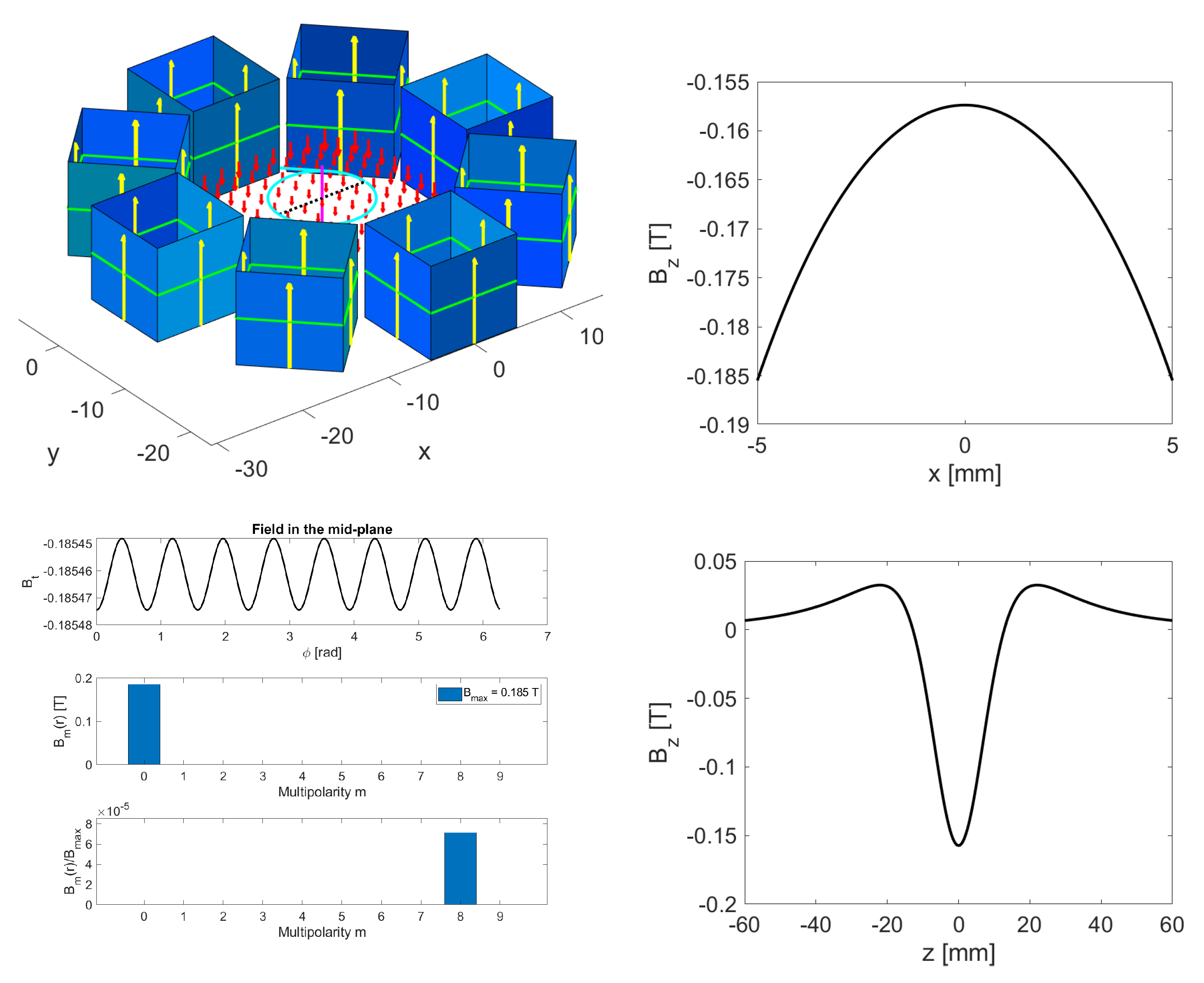
It turns out that the frame for the quadrupoles can also be used to construct both axial and radial solenoids; for an axial solenoid, we only have to insert all cubes with their easy axis pointing along the
z-axis. The top-left image in
Figure 4 illustrates this. Note also the black dotted line and the cyan circle in the midplane as well as the solid magenta line to illustrate the
z-axis. The top-right plot shows the
z-component
of the magnetic field in the midplane along the black dotted line visible on the top-left image. We see that it has a parabolic shape—the magnitude of the field closer to the permanent magnets is higher. We see that
points opposite the direction of the easy axis of the cubes and reached about
T in the center of the assembly. On the lower-right plot, we also observed that
, after being negative in the center of the assembly, became positive with a magnitude of 0.03 T around
mm. On the three-panel image on the bottom-left, we explored the impact of approximating the solenoid by eight cubes. The upper panel shows
in the midplane of the assembly around the cyan circle, which had a radius of 5 mm. We observed eight oscillations as we moved around the azimuth
, whose amplitude, however, was rather small—less than
times the magnitude of the average
, which was
T at
mm. We conclude that, even though the field quality is limited, constructing solenoids is feasible within our framework.
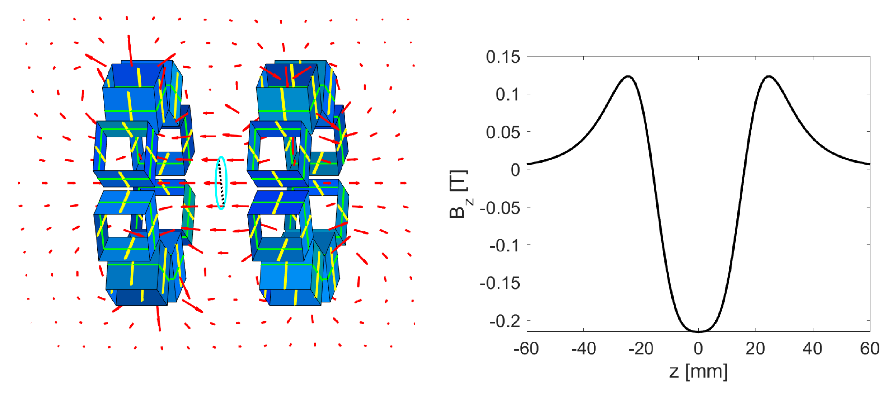
Likewise we can construct a radial solenoid by rotating the cubes such that their easy axis either points inwards or outwards, and we can construct one solenoid from two rings, separated by 20 mm, as shown in
Figure 5. The easy axes of the left eight-cube rings point inward, and those of the right ring point outward. The magnetic field is illustrated by the red arrows and points from the right towards the left assembly along the negative
z-axis in the intermediate region. The plot on the right-hand side in
Figure 5 shows
along the
z-axis, where
corresponds halfway between the two assemblies whose position is indicated by the blue dashed boxes. We see that the maximum value exceeded 0.2 T in the center and and reached about 0.12 T just outside the two assemblies. The homogeneity of the field was comparable to that of the axial solenoid close to the cubes and was better in the intermediate region.
6. Adjustable Dipole
Inspired by the observation that the fields of two very short magnets with opposite polarity almost cancel and the fact that the fringe fields of the dipole from
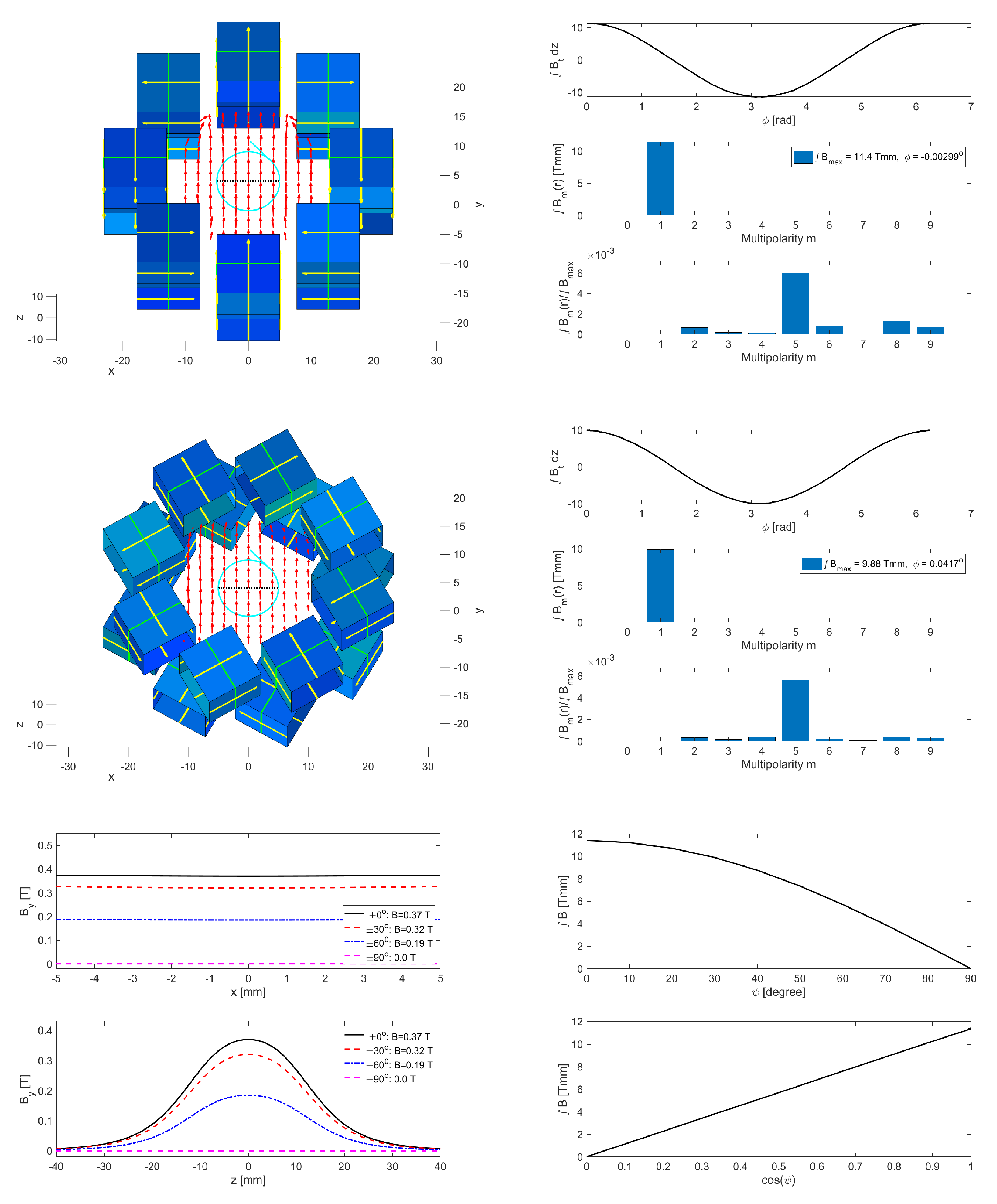
Section 3 extend far beyond the physical length of the magnet, we placed two dipole rings very close to each other (2 mm between the rings) and then rotated one with respect to the other. The images on the left-hand side in the top and middle row of
Figure 6 illustrate the geometry of these assemblies. On the top left, the two eight-cube rings were aligned, and the one below the upper ring was rotated by
counter-clockwise, while the lower ring was rotated by
clockwise.
The three-panel images towards the right of the respective geometries illustrate the integrated multipole content of the assemblies. In the upper panel on the top-right image, we see that the tangential field component of the field integral showed a sinusoidal pattern that was responsible for the dominant dipole component visible on the middle panel. The integrated strength of
Tmm of this assembly was twice that of the single magnet from
Figure 2, because the fields superimpose linearly in ideal permanent-magnet assemblies. Furthermore, the lower panel shows that the dominant higher multipole was the decapole (
) component whose contribution was
smaller than the main component. The right-hand image in the middle row shows the integrated field of the assembly with the two rotated magnets. The tangential field shown on the upper panel was also sinusoidal, albeit with a reduced amplitude of
Tmm, which is also given in the legend of the middle panel with the Fourier-harmonics. Even in the rotated geometry, the dipole contribution was dominant, and the relative contributions of the unwanted harmonics, shown on the lower panel, were below
.
That the dominant effect of rotating two eight-cube magnets with opposite angles only changed the integrated field from to Tmm but did not adversely affect the unwanted multipoles encouraged us to explore the dependence of the field integral for different rotation angles . The image on the left-hand side in the bottom row shows the vertical field along the z-axis on the lower panel for and . We see that rotating the two eight-cube rings reduces the peak field in the center of the magnet from T down to zero. The upper panel shows on the x-axis along the black dotted line, and we see that the field was rather constant—only the amplitude was different for different values of . The lower panel shows the fringe fields of along z for the four values of .
Finally, we systematically varied
in steps of
and showed the integrated field component (or the amplitude of the Fourier harmonic for
) as a function of
on the upper panel in the image on the right-hand side in the bottom row of
Figure 6. We observed that the integrated field decrease in a smooth curve from 11.4 Tmm down to zero at
, where the easy axes of cubes on top of each other have opposite polarities and cancel one another. On the lower panel, we show the same data but plot versus
instead. We found that now the integrated field strength shows a linear dependence on
, which indicates that the integrated field is given by twice the integrated field of one eight-cube ring times
. However, this is just the projection of the maximum field of the rings onto the vertical axis. The field components along the vertical axis add, but along the horizontal axis they cancel. This will make tuning and setting up of such double-dipole assemblies rather straightforward.
7. Adjustable Quadrupole
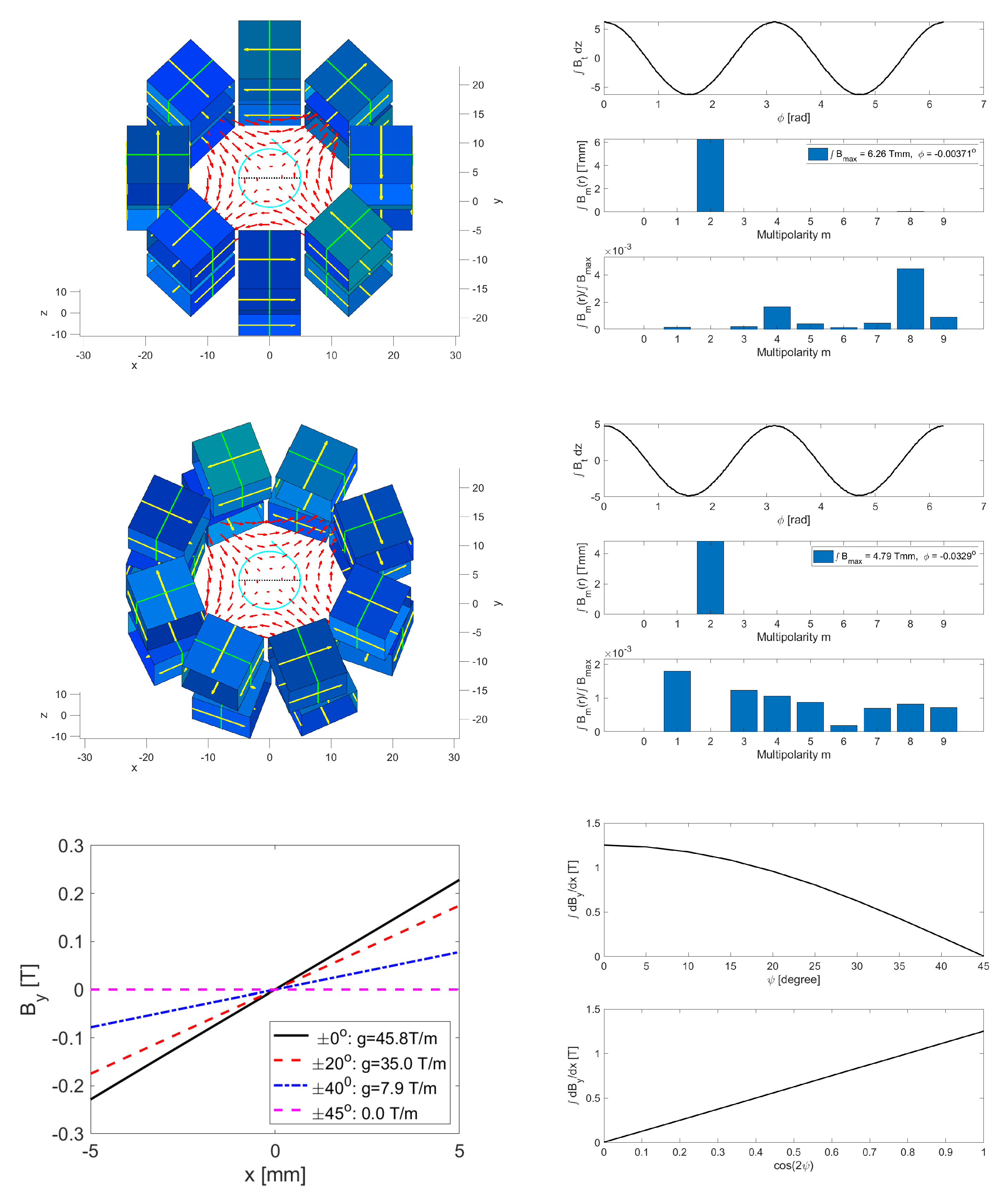
It is certainly no surprise that the same idea also works with quadrupoles. On the top-left image is
Figure 7, in which we show the geometry of two aligned (
) eight-cube quadrupoles on top of each other with a 2 mm space between the rings. On the image on the middle row below, we show the same assembly, but the upper ring is rotated by
and the lower ring by
. The images towards the right of the geometries show the tangential field on the upper panel, the Fourier harmonics on the middle panel, and the relative magnitude of the unwanted harmonics on the bottom panel. We observed that the dominant harmonic was the quadrupolar
with integrated strength, evaluated at a radius of 5 mm, going from
Tmm for
to
Tmm for
. The harmonics in all cases were smaller by a few times
.
Next, we systematically changed
in steps of
from
to
and showed the gradient on the mid-plane (indicate by the black dotted line) on the lower-left image in
Figure 7. We see that the gradient changed from
T/m for
to zero at
. On the right-hand image on the bottom row, we plotted the integrated gradient
as a function of
in the upper panel. We see that it moves smoothly from
Tmm
mm
T for
to zero at
. On the bottom panel, we plotted the same data versus
and found a linear dependence of the integrated gradient on
, which will make tuning and setting up double-quadrupole assemblies straightforward.
8. Some Applications
Here we discuss three examples where the strap-on magnets might prove useful: a small chicane, a triplet cell, and a solenoid lens. Let us start with the chicane.
8.1. Chicane
Four-dipole chicanes are frequently used in accelerators to provide an energy-dependent path length for a beam, which helps to compress beams longitudinally [
2,
10]. The figure of merit for a bunch compressor is the
, where
L is the distance between the outer and the inner two dipoles, and
is the deflection angle of one dipole. This angle is given by the ratio of the integrated field
of the dipole and the momentum of the beam, often expressed through its rigidity
. For a beam with momentum 300 MeV/c, the rigidity is about 1 Tm, such that the variable two-magnet dipole from
Section 6 with an integrated field of
Tmm deflects a 300 MeV beam by 11.4 mrad. With
m between the dipoles, we therefore deflected the beam by about 5 mm and stayed within the region shown on the bottom left in
Figure 6. Furthermore, we found
mm. Since we can adjust the magnetic field by rotating the two adjacent dipoles, we can adjust the
between the maximum value and zero.
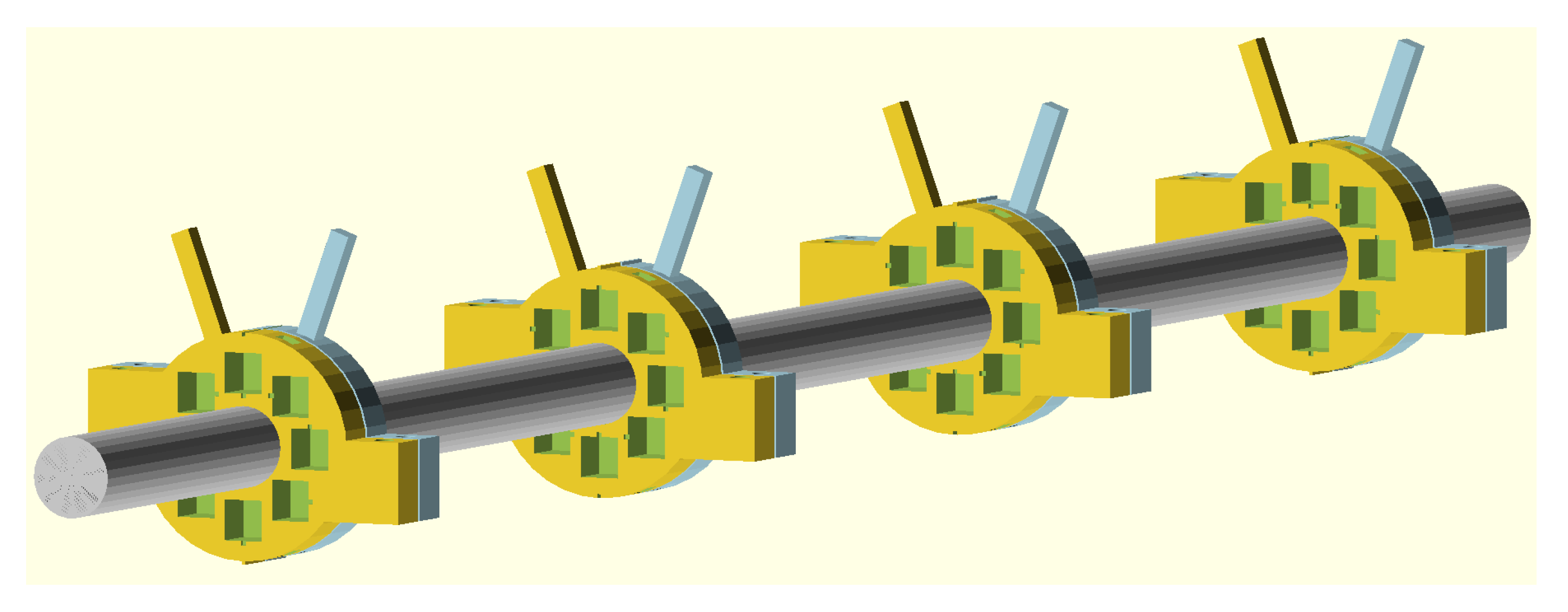
Figure 8 illustrates such a chicane with four variable dipoles wrapped around the grey beam pipe. One of the magnets was colored light blue and had a handle attached sticking out to the top right, while the other magnet was colored yellow and had a handle sticking out towards the top left. The handles were attached to the 5 mm square holes on the periphery of the frames, which is also visible on
Figure 1. Moreover, careful inspection shows that the two middle assemblies have opposite polarity (the central ones have a notch sticking out at the top, while the outer ones have a groove), such that they deflect a beam in opposite directions. Connecting all yellow handles with a rod allows to change the rotation angle of all yellow magnets by the same amount, while a rod connecting the light blue handles rotates all light blue magnets by the same amount, which permits to change the excitation of all dipoles synchronously. Small variations in the excitation of different magnets can be compensated by placing small plates between the handles and the connecting rod. Note that for the illustration in
Figure 8 the distance
L was reduced to 0.2 m.
8.2. Triplet Cell
In beam lines where long stretches of free space between magnets as well as round beams are required, often triplets are used. They are combinations of three closely spaced quadrupoles where the first and third quadrupole are excited equally, and the center quadrupole has opposite polarity and twice the excitation.
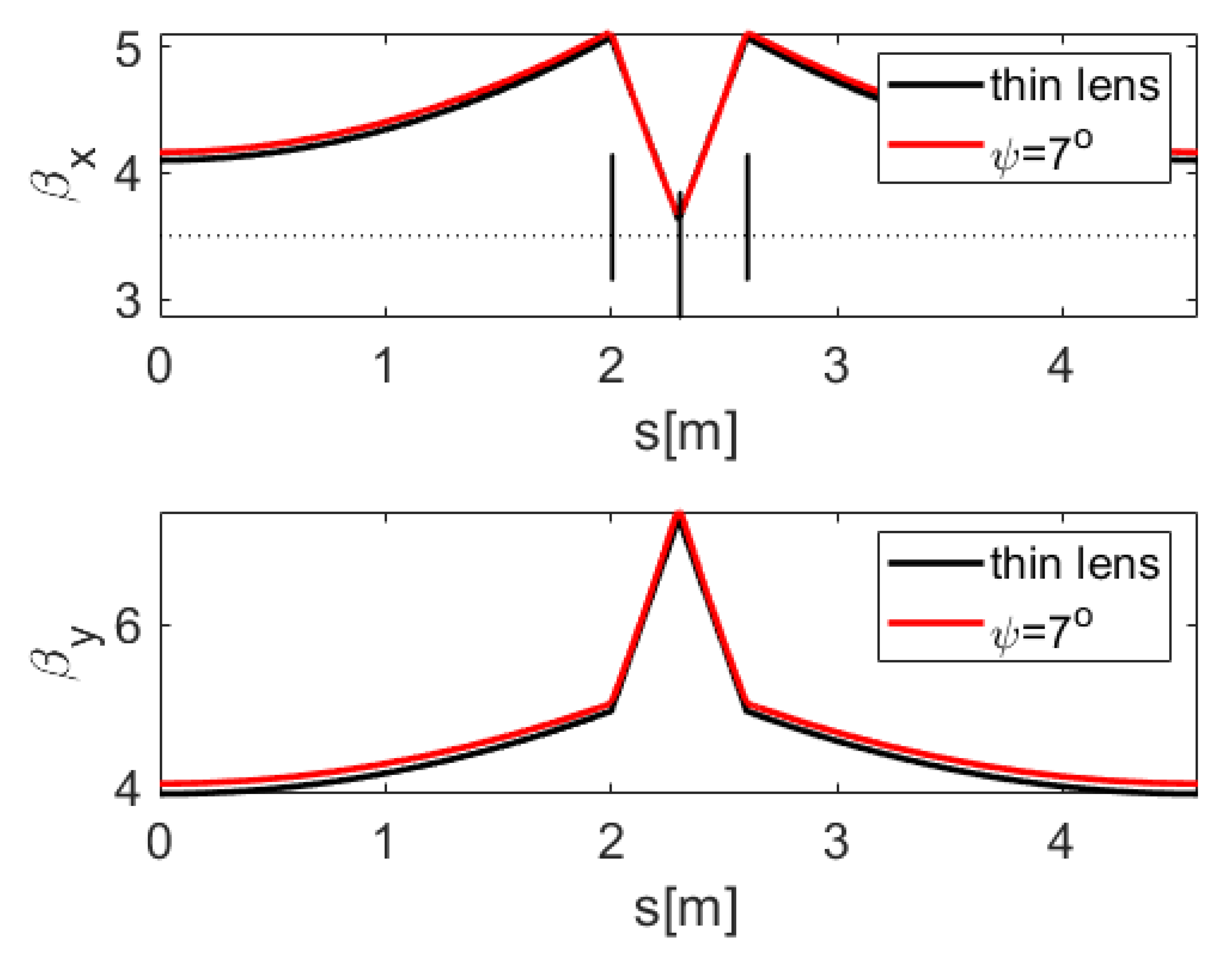
Figure 9 shows the magnet lattice with the three thin-lens quadrupoles and the horizontal beta function
in the upper panel and the vertical beta function
in the lower panel. The black lines show the beta functions for the thin lens model with a betatron phase advance per cell of
in both planes. Note that the magnets are only located over a distance of 0.6 m such that there is almost 4 m free space available between magnets of adjacent cells.
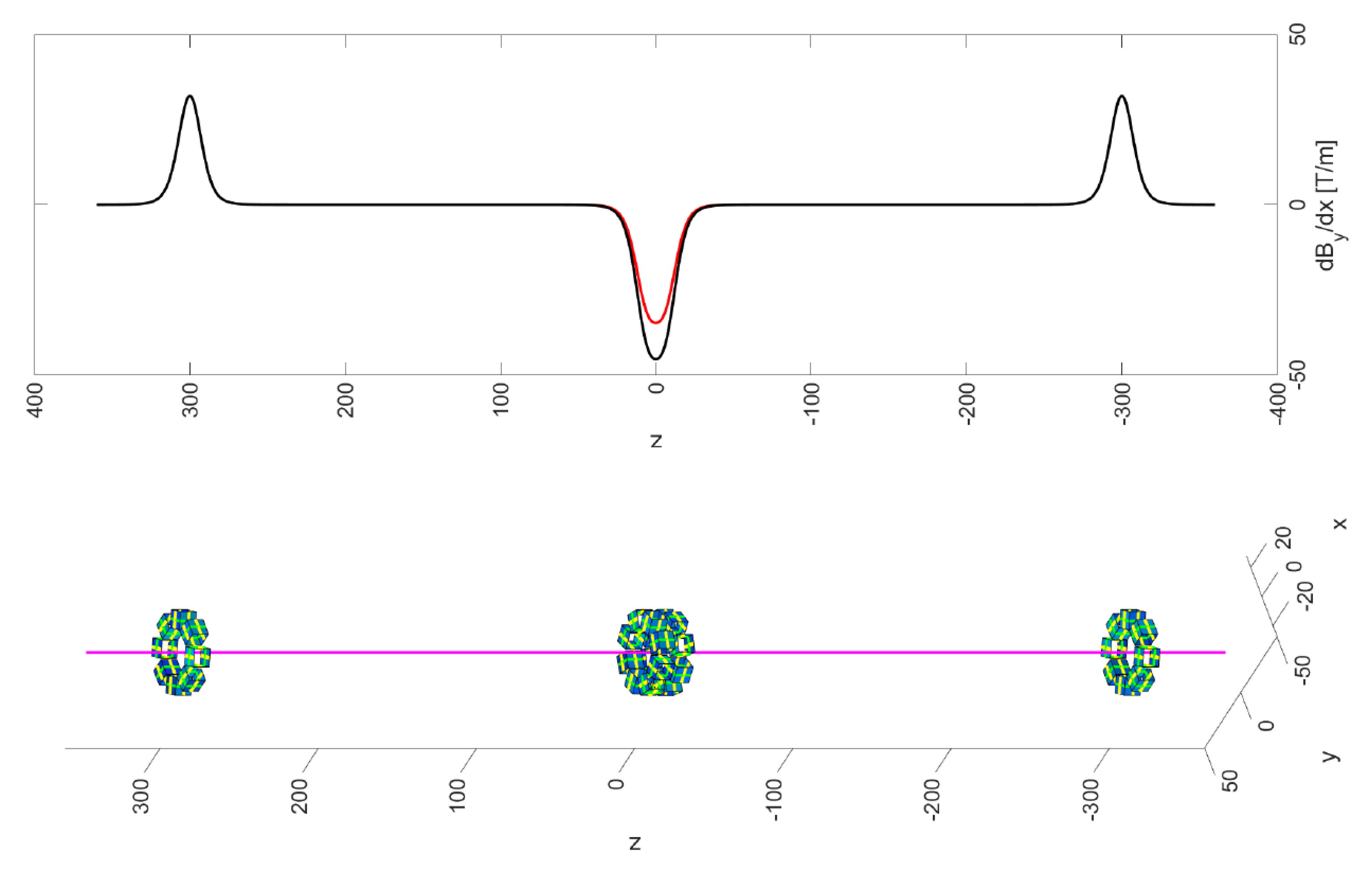
Our quadrupole rings are particularly attractive to realize such triplets; we used a single ring for the two outer quadrupoles and two rings, rotated by
, for the double-strength center quadrupole with opposite polarity. The lower image in
Figure 10 shows the two outer rings located near
mm and the inner double-ring near
mm. The magenta line denotes the axis on which beam travels. We point out that adjusting the relative rotation angle
between the two center quadrupoles gives us some tunability. The upper image in
Figure 10 shows the gradient along the beam axis. Note the opposite polarity of the outer and inner quadrupoles. Moreover, the black line shows the field for
and the red line for
.
We then empirically adjusted
; calculated the gradient along the beam axis; automatically wrote a beam-line description, consisting of many 1 mm long quadrupoles; and calculated the beta function with software from [
2]. With
, we found that the phase advances were close to the
for the thin-lens lattice. The red lines in
Figure 9 showed
and
for the gradients produced by our quadrupole rings, which agreed very well with those of the thin-lens model, shown in black.
8.3. Solenoid Focusing
The radial solenoid from
Section 5, whose geometry and field are shown in
Figure 5, is suitable to focus round low-energy beams. In the upper panel of
Figure 11, we show the beam envelope of a 5 MeV electron beam with a normalized emittance of
m rad passing through two such radial solenoids spaced 1.75 m apart. On the lower panel, we recognize
from the right-hand image in
Figure 5—once near
and once near
m. The envelope was calculated from
by numerically integrating the paraxial-ray equation [
11]. The initial beam was parallel and had a radius of 1 mm but then developed a focus near
m, which is consistent with the focal length
f calculated from
m, where we had
T
m and
Tm for the 5 MeV beam.
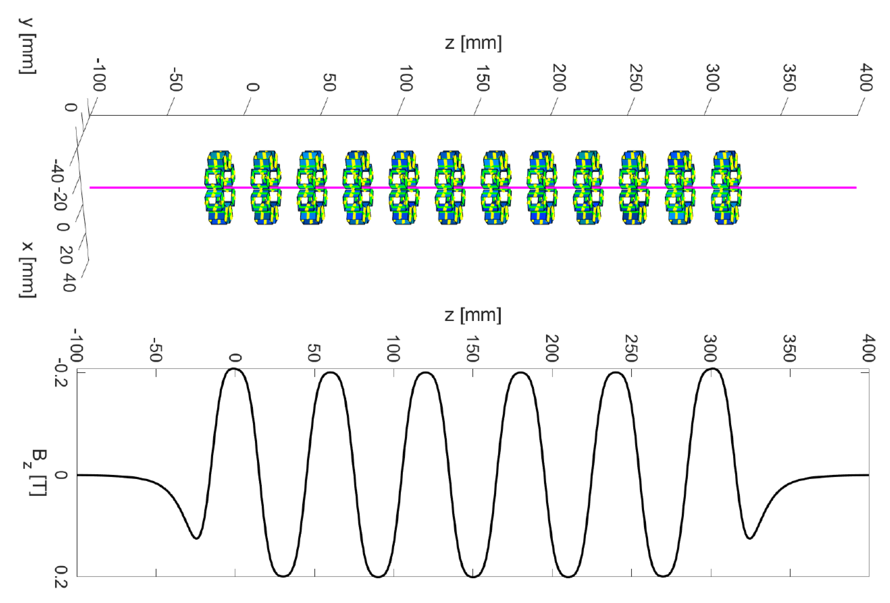
Making the solenoid stronger is a simple matter of repeating multiple copies of the radial solenoids, as shown in
Figure 12, where six copies of the solenoid from
Figure 5 follow with equal distance between consecutive rings. Note that the polarity alternates from one ring to the next. The upper panel shows the beam axis in magenta together with the twelve radial solenoids with alternating polarity, whereas the lower panel shows the longitudinal component
on the beam axis. Note that the rings are placed every 30 mm, and the amplitude of
reaches
T. The integrated focusing strength
was
T
m for this configuration. This configuration would work for a 13 MeV electron beam (
Tm) where it leads to a comparable focal length close to 0.9 m.
9. Scaling
We point out that changing the value of the remanent magnetic field will just scale the field values reported in the remainder of this report accordingly.
Moreover, changing the linear dimensions, the size of cubes w, their radial position o, and the size of the frame, will keep all quantities, whose dimension is Tesla, unchanged. For example, the field in a dipole made of 5 mm cubes equals that of a dipole made of 10 mm cubes, but its fringe field does not extend as far as that of the bigger dipole. Therefore the integrated field of the smaller magnet is a factor of two smaller. Likewise, the integrated gradient of a quadrupole made of 5 mm cubes is the same as that made of 10 mm cubes. In the smaller magnet, the gradient is doubled, but the total length is halved.
10. Conclusions
Based on the analytic results for the magnetic fields from permanent magnets from [
3], we explored the use of permanent-magnet cubes to create dipoles, quadrupoles, and solenoids. All examples were based on the frames for 10 mm cubes, shown in
Figure 1, but are easily scalable to use cubes of a different size, to include more cubes or to produce other multipoles. We found that the magnets have reasonably good field qualities; the amplitudes of the harmonics at a radius of 5 mm in all cases were less than a fraction of a percent and often better.
An attractive feature is the possibility to retrofit these magnets to existing beam lines without having to open the vacuum system; the two magnet halves are simply strapped-on to the beam pipe. A second attractive feature is the possibility to combine two closely spaced rings to obtain dipoles and quadrupoles whose strength is continuously adjustable, while their field quality is comparable to that of a single ring.
Finally, we found these magnet rings suitable to construct beam-line modules for chicanes, a triplet cell, and solenoids focusing a low-energy beam.


