1. Introduction
Condition monitoring [
1] is an emerging engineering area which is developing rapidly with the help of available sensing technologies, providing the means for efficient asset management and predictive maintenance in industry and infrastructures [
2]. In this context, structural health monitoring (SHM) is of great importance for the management of physical infrastructures, also providing information for early damage prognosis [
3]. While a number of sensing approaches have been employed in SHM, the photonic and optical fiber sensing technology [
4] has been established lately as a very promising solution as it provides many favorable characteristics, enabling the flexible placement or incorporation of lightweight optical fibers in the monitored infrastructures [
5]. Such photonic solutions can be tailored for SHM from small and medium scale [
6] to large scale systems by distributed fiber optic sensors [
7].
Distributed optical fiber-based sensing is ideally suited for several applications beyond to structural health monitoring (SHM) [
8,
9], such as train location and speed detection [
10], intruder detection [
11], seismic alert and study [
12], safety and anti-theft pipelines (gas-duct and petrol lines) [
13,
14], etc. Indicatively measuring the strain of a fiber attached to a rail of a high-speed line, it is possible to obtain the dynamic load (weight-in-motion) of a train or to determine the pressure and fluid flow in a pipeline with a non-intrusive measurement. Considering the installation of a dedicated sensed optical fiber, the available applications multiply—it can be used to monitor nuclear power plants, in order to know if structural damages are approaching before leakage occurs or for control of intrusions in a wide area, from military to security context.
Distributed fiber optic sensing can rely on a number of different intrinsic physical phenomena in the optical fiber medium such as Rayleigh, Brillouin and Raman scattering that result from the interaction of propagating photons with local material properties like density, temperature and strain [
7]. The specific approach of phase optical time-domain reflectometry (Phase-OTDR) examined here relies on the detection of changes of Rayleigh scattered light in optical fibers, induced by external environmental factors that are being monitored. Rayleigh scattering is generated by small random inhomogeneities in the optical fiber medium, which result in microscopic refractive index fluctuations and act as scattering points for the propagating light [
7]. External temperature changes or mechanical stress applied to the fiber induce changes in the Rayleigh scattered light. Phase-OTDR systems perform optical signal analysis on the Rayleigh backscattered light, a small portion of the total Rayleigh scattered light which travels in all directions and is already small for standard silica fibers, to retrieve information about the environment of the optical fiber. The backscattered signal is generated using highly coherent pulses of laser light, introduced in one end of the optical fiber (origin of the fiber), and is detected by a photodetector at the same end. Since Rayleigh scattering is a linear optical effect, the backscattered light maintains the coherence of the incident light, generating at the detector an interferometric sum of all partial backscattered contributions from different fiber scattering centers within the pulse width. As the light pulse travels along the fiber, we monitor the Phase-OTDR signal for each position of the pulse in the fiber. The position of the pulse is known by the speed of light in the fiber and the time of acquisition after the pulse launch. Therefore, a Phase-OTDR trace represents the interferometric (amplitude and phase) sum of multiple and random light scattering centers in the fiber, as a function of fiber position. The resulting trace is typically a random, noise-like pattern that remains same over time if the scattering centers do not suffer from any changes. Any mechanical stress (e.g., positive or negative strain) or temperature change at one certain location will generate an amplitude change in successive Phase-OTDR traces at the disturbance location. By repeatedly interrogating the optical fiber with successive laser pulses, it is possible to know at which point of the fiber a change of state happened by tracking the difference between unperturbed and perturbed Phase-OTDR traces. In this way, the optical fiber becomes a long, distributed sensor, providing almost instantaneous information about the change of strain or temperature along a length of several km.
Strain and temperature are also measured for SHM applications by point sensors, such as optical fiber Bragg gratings (FBGs) [
15] and electric strain gauges [
16], largely used in accelerometers, geophones and displacement sensors. Point sensors can exhibit very high performance in monitoring a specific point, but sometimes they are bulky, and they need several installation points in order to interrogate a large structure. For Phase-OTDR systems, the relation between strain (or temperature) and the backscattered signal is linear only at low-intensity light levels [
17], as non-linearity appears for increased intensity. While most simplified Phase-OTDR systems are suitable for locating a perturbation and pattern/harmonic detection [
18], more sophisticated setups can also measure strain and temperature. Such Phase-OTDR systems, which employ techniques such as coherent detection [
19] and chirped pulses [
20], can exhibit high performance at very high frequencies of perturbation [
21], allowing a direct comparison with well-established point-sensing technologies. Other distributed sensors, suitable for SHM, include Brillouin optical time-domain analysis sensors (BOTDA) [
22] and Raman-based sensors [
23]. BOTDA sensors can provide strain and temperature measurements with, e.g., a spatial resolution of 2 m and a temperature uncertainty of 1.2 K over 100 km [
24], but they require a large number of acquisitions to reduce noise through averaging, which makes the measuring interval several minutes long. Raman-based sensors are suitable for slow measurements, and they have reached resolutions of 17 m and 5 K (length and temperature, respectively) over 40 km [
25], with measurement times several minutes long. Currently, Phase-OTDR is the only distributed technology that allows real-time measurements at a high frequency where the only limitation of the interrogation rate is the fiber length. Raman and Brillouin based technologies are shown to be extremely accurate with specific well-tuned setups, and they are therefore perfectly suitable for the static analysis of strain and temperature (Brillouin) or temperature (Raman) in large and small structures. On the other hand, Phase-OTDR can be considered as the most appropriate choice for the wide-band dynamic analysis of strain and temperature in similar structures.
Currently, sophisticated Phase-OTDR systems with a linear response to external perturbations are high-cost, bulky, cross-interfering as well as temperature and alignment sensitive; therefore, their use in sensing applications is strongly limited. On the other hand, there are many applications where simple non-linear Phase-OTDR systems can provide useful distributed information for vibration source location and spectral pattern recognition (determination of the kind of vibration source). In these cases, a low-cost, versatile, reliable, fast Phase-OTDR system is preferable. Non-linear Phase-OTDRs have some limitations; spectral analysis (spectral footprint recognition of a vibrational event) is moderately complicated by a non-linear response, and the signal of a specific point (position of the fiber) can suffer from a statistical response fading [
26]. Such an uncontrolled signal change increases the difficulty in setting event alarm trigger thresholds when the signals are particularly noisy. Even with these limitations, non-linear Phase-OTDRs are useful instruments for SHM, where an extended sensing fiber length becomes essential for frequency analysis, aging detection or damage prevention on any large civil structure [
13].
Without proper engineering non-linear OTDRs remain relatively expensive due to the intrinsic need for high-performance components. Typical laboratory setups use kHz-linewidth lasers, GHz-modulators, several optical amplifiers, highly sensitive photo-detectors, high bandwidth amplifiers and high-sample-rate/high-bandwidth digitizers. This set of components, together with assembling costs and tuning difficulties, make Phase-OTDR a niche technology that struggles to spread in applied research and real-life applications, such as SHM, even though its cost is small when considered per length of sensing. Typical costs for laboratory assembling of fast Phase-OTDR systems range between 100 and 500 k€, while “low-cost” commercial Phase-ODTR systems are available in the 250 k€ range.
According to
Table 1, all distributed monitoring technologies are capable of providing useful information for similar applications, and therefore the choice of technology should be based on the required analysis, sample rate, resolution, monitored parameters and cost. For example, a static analysis of a large structure obtains accurate and low-cost temperature information from Raman-based systems, while accurate strain information requires more complex systems based on Brillouin and Phase-OTDR technologies.
In this work, we present the design and implementation of a simple, low-cost, alignment-free, and sensitive non-linear Phase-OTDR system, designed to be portable and harsh-environment tolerant. The cost of the proposed instrument is under 10 k€, including the acquisition device and excluding the optical fiber, the length of which depends on the application. The low-cost Phase-OTDR system is capable of vibration location, frequency analysis and spectral pattern/harmonic recognition. The instrument is the result of efficiently using low-cost components commercially available for the telecommunication industry. The proposed design has the potential to increase the spread of Phase-OTDR technology in numerous applications.
The paper is organized as follows:
Section 2 presents the minimum requirements and specifications of the proposed system describing the operation principle of Phase-OTDR together with the design guidelines and the current constraints.
Section 3 shows the design of the system and its architecture based on suitably identified discrete components.
Section 4 details the electronic implementation of the designed system together with the precautions used to keep the highest performances possible.
Section 5 presents the interconnection and integration of the system in a single unit, also discussing packaging issues.
Section 6 discusses the theoretical performance and the expected spatial resolution of the developed system. Finally,
Section 7 presents some preliminary experimental results relating the performance to the theoretical resolution.
2. Minimum Requirements and Specifications
There are three essential specifications to be set for a dynamic, non-linear Phase-OTDR system: (1) the sensing range (the length of fiber that the system can interrogate successfully for vibration detection), (2) the spatial resolution (the minimum distance between two separate events that the system can discriminate as being separate), and (3) the maximum interrogating sample rate [
27]. The sensing range, as it is shown in
Section 3 and depicted in detail in
Table 2, has a strict correlation with the required signal-to-noise ratio (S/N ratio) of the retrieved signal; e.g., the S/N ratio for a 5-km fiber is 15.7 dB. The spatial resolution, as shown in detail in
Section 6, depends on the laser pulse duration, among other things. We employed 50 ns laser pulses, which resulted in a spatial resolution of 5 m (determined experimentally in
Section 7). The maximum sample rate of the system is limited by the analog to digital converter (ADC) and the overall system bandwidth, and also by the fiber length. This is because the duration of the backscattered signal (track signal duration,
Ttrack) is:
where
L is the fiber length,
v =
c/
neff the speed of light in the fiber,
neff the effective refractive index of the fiber (typically ~1.5), and
c the speed of light in vacuum. The duration of the backscattered signal is such because each point in the fiber generates a backscattered contribution after it is reached by the interrogating light pulse and each backscattered contribution must travel back to the origin of the fiber to get detected. For practical use, assuming
, Equation (1) is simplified in:
a delay of at least
Ttrack before introducing a new pulse of light in the fiber is necessary to avoid overlapping signals from consecutive interrogating pulses. Therefore,
Ttrack defines the maximum interrogation rate of the fiber, and the repetition frequency with which the optical fiber is interrogated (
ftrack rate, track interrogation rate) must satisfy:
From Equations (1) and (3), we observe that the maximum interrogation rate depends on the length of the fiber:
Therefore, a 20 km long optical fiber allows a sample rate of 5 kHz, which, according to the Nyquist theorem, allows capturing vibrational frequencies as high as 2.5 kHz.
Because fast data sampling generates a significant data flow, the use of industrial computers is ideal, such as those based on the PXI (PCI eXtensions for Instrumentation) platform. To enable the use of standard computers, instead, we employed a relatively inexpensive USB3 digitizer with 200 MHz bandwidth. Therefore, we set the bandwidth of the entire system to this value (200 MHz). With a 50-ns laser pulse and a 5-m spatial resolution, the required bandwidth is mostly below the designed 200 MHz value [
28] (more details in the performance analysis in
Section 6).
3. System Design
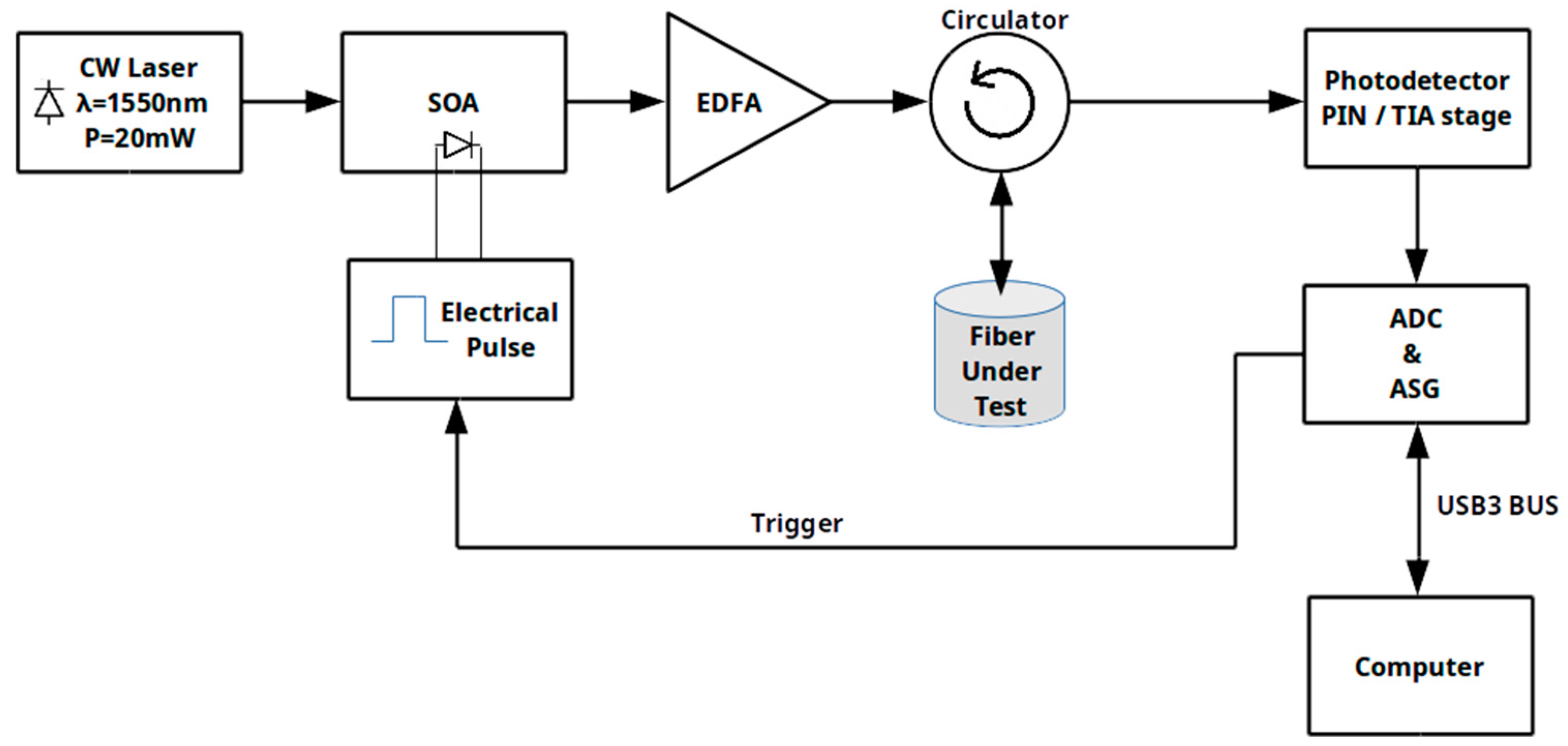
The system design is shown in
Figure 1. The continuous wave (CW) diode laser output is pulsed by a semiconductor optical amplifier (SOA) used as a shutter. The SOA is driven by electrical pulses of current (500 mA) for a duration of 50 ns. The pulse rise/fall times are on the order of ns. The laser output power is higher than the saturation optical input power of the SOA, resulting in narrowing of the SOA linewidth from MHz to kHz values due to spectral hole burning (SHB) [
29]. Therefore, the SOA is used solely for pulsing and spectrum shaping the CW laser, and it does not contribute to the optical pulse amplification. Taking advantage of the SHB effect, we were able to use a low-cost laser (with a bigger linewidth) achieving about one order of magnitude cost reduction on this component. The SOA is also a more affordable solution for pulsing light, compared to other modulators or shutters, providing more than one order of magnitude cost reduction for pulsing. Even though an SOA requires higher driving current than other interferometric modulators for light pulsing (e.g., acousto-optic or electro-optic modulators), the latter are more expensive, and they need relatively high and tuning-sensitive operating voltages, also increasing the complexity and cost of the accompanying electronic control board. Interferometric modulators can provide a higher extinction ratio and greater linearity compared to SOAs, but, in this application, the SOA extinction ratio is reasonably good, and linearity is not a critical requirement (as indeed SHB is a desired non-linear effect).
The erbium-doped fiber amplifier (EDFA) provides the necessary amplification to reach ~400 mW of peak pulse power. A typical Phase-OTDR system includes one or two filter blocks to reduce both the EDFA amplified spontaneous emission (ASE) noise (at the output of the EDFA) and the DC signal component that arrives at the PIN photodiode. In this design, we tuned the system optical power and the trans-impedance amplifier (TIA) stage to keep the ASE noise low with respect to the signal amplitude. The EDFA, the circulator and the PIN photodiode are low-cost, widely available, standard telecommunication devices. The PIN is an InGaAs photodiode with a bandwidth of 3 GHz, a maximum responsivity of 0.95 A/W (at 1550 nm), a capacitance of 0.5 pF at Vr = −5 V and an FC/APC connector. The ADC has an arbitrary signal generator (ASG) that works as an arbitrary trigger for the electrical pulse generator of the SOA. The computer interface allows for setting the track interrogation rate, the sample rate and the number of samples per track. These on-fly settings allow an immediate change of the interrogation parameters and instantaneous adaptation to different lengths of the optical fiber and SHM needs.
Even though the combination of the EDFA, the PIN photodiode and the TIA, allows a length of sensed fiber beyond 20 km, the low-cost digitizer (8 bits ADC) poses some limitations for long lengths of fibers. The ADC is a low-cost wide-bandwidth device with an effective resolution below 8 bits, reduced by the calibration, the saturation values, and the value distribution. It allows 213 values corresponding to an effective resolution of about 7.7 bits and, as we will show later, with a noise level around 1.6 bits. Under those conditions, in-fiber attenuation creates an essential difference between the signal beginning and end. For example, a sensed optical fiber of 25 km provides 10 dB of attenuation, which makes the backscattered signal ten times weaker at the end than at the beginning. Assuming the beginning of the signal is perfectly set to the ADC range, at the end the signal will present an ADC resolution reduction more significant than 3 bits (~3.3 bits). Therefore, for the end of the signal, the nominal 8-bit ADC behaves like a 4.4-bit ADC, corresponding to 21 levels of discrimination with 1.6 bit of noise. The corresponding S/N ratio, at 25 km, becomes 8.5 dB. Finally, it should be taken into account that the TIA cannot be set to keep its output dynamics entirely in the voltage range: to maintain linearity and fast recovery time from saturation, it is necessary to add some margins. Those margins cause, even in the best case as described later in
Section 4, about a quarter of a bit of resolution reduction, while this value is typically between half and one bit. In this case, at the end of the 25 km fiber, the ADC has about 18 significant discrete values, i.e., 4.2 effective bits, and an S/N ratio of 7.7 dB.
Therefore, the sensing range should be specified together with the S/N ratio because the range depends on the sensitivity required by the application. According to
Table 2, for a range of 5 km, the S/N ratio is 15.7 dB, while for a 10-km range, the S/N ratio is 13.7 dB.
4. Electronic Design
As we stated above, the electronics are designed to meet the 200 MHz system bandwidth while the PIN photodiode bandwidth is 3 GHz. The photodiode was carefully chosen since it is one of the most critical elements. The TIA block is designed with a bandwidth which limits the noise generated by the first stage and, at the same time, does not cut off high-frequency signal components. Indeed, an inappropriate TIA bandwidth can degrade the entire system performance. An essential point is the balance between bandwidth and amplification gain. It is well-known that increasing the gain typically leads to a bandwidth reduction. A method that mitigates the bandwidth reduction is the combination of several amplification stages. However, a long series of different amplification stages leads again to a global bandwidth reduction [
30]. When a high gain is required, it is good practice to split the gain into 2–3 stages to effectively control both the bandwidth and the gain. Another critical point is that signal cables must be avoided when possible. Otherwise, cables must be equalized to compensate for losses and bandwidth reduction, and an equalized (compensated) cable must be treated as a lossy cable, which implies it could be necessary to modify the amplification factors in the entire system.
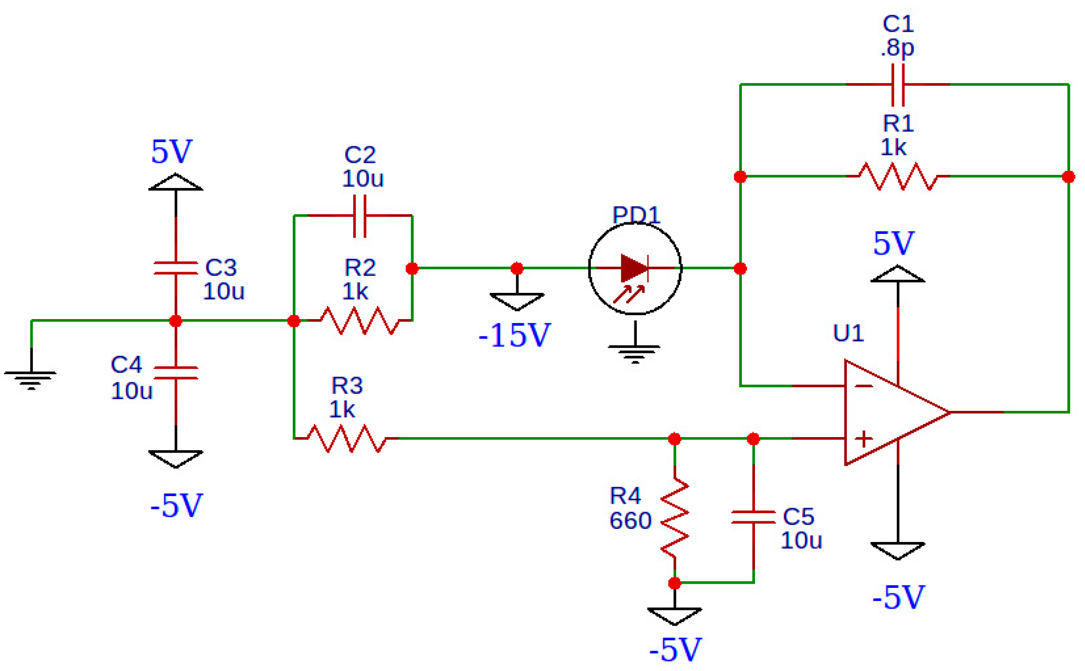
As shown in
Figure 2, we use a TIA to convert the small retrieved photodiode current to a wide range of voltages. The TIA output voltage is limited by the power supply voltage and by the saturation limits of the operational amplifier.
The TIA block is made using a voltage feedback operational amplifier with a G = 1 bandwidth of 3.9 GHz (OPA-847) in a trans-impendence configuration to get a closed-loop bandwidth above 300 MHz with a gain of 1kΩ (1000 V/A). The bandwidth (BW) is calculated as:
where
GBWP is the gain-bandwidth product,
RF is the trans-impedance amplification (feedback resistor), and
Cin is the total input capacitance (sum of PIN photodiode capacitance and common and differential mode capacitances). Since the ADC digitizer has a bandwidth of 200 MHz (Picoscope series 3000 digitizer, model 3206D, 8 bit, 1 GS/s), it is essential that the input signal has a higher bandwidth (300 MHz) to maintain the 200 MHz bandwidth target almost unchanged. Indeed, in the case of N cascaded stages with a bandwidth
BWstage each, the overall system bandwidth
BWSystem is degraded according to the following equation [
31]:
The TIA amplifier is designed to have a negative output offset (about −3 V at no input) to allow better usage of the available range of the ADC digitizer. This innovative TIA operation enables a digital resolution increase of about one bit. Level adaptation is a typical case where the design fails to achieve high vertical resolution and speed (bandwidth). The negative voltage is set to maintain a fast recovery time from saturation (and therefore kept far from the maximum absolute input voltages). The PIN photodiode is operated with a reverse voltage of −12 V to decrease its capacitance and increase its speed.
The TIA power supply is a linear one, specifically designed to have very low noise, while the EDFA, a high current demanding device, uses a switching power supply. In the specific case of the EDFA, we use a low noise (below 10 mV) switching power supply since the EDFA control board has efficient internal control and a stabilizing circuit. During development, it is crucial to check if the switching power supply introduces noise somewhere in the system. The laser module is mounted on a heat sink board, and it is stabilized with temperature and power controllers that use a low-noise power supply. The laser power controller is an overvoltage-protected current generator (current stabilized) made with LM317 (adjustable linear positive voltage regulator).
To conduct a proper differential Phase-OTDR analysis of the optical fiber state, it is critical to use a train of light pulses as similar as possible. This is because the backscattered OTDR signal depends on the input light signal, as the interference pattern changes completely by changing any input light property, such as the pulse shape, coherence, bandwidth, frequency, polarization, etc. For this reason, it is essential to use laser sources with a high degree of coherence and stabilization together with a precise pulse generator and stable temperature and power controls. The laser and SOA are both temperature-stabilized with a separate temperature controller circuit for each, which uses their internal thermistor to read the temperature and their internal thermo-electric cooler (TEC, a Peltier element) to sink or produce heat. The schematic of the temperature controller, shown in
Figure 3, is current limited and has two indicator LEDs for heating (red LED) or cooling (blue LED) operation. If the system operates at an ambient temperature below 0 degrees or above 40 degrees, then the corresponding LED remains constantly on.
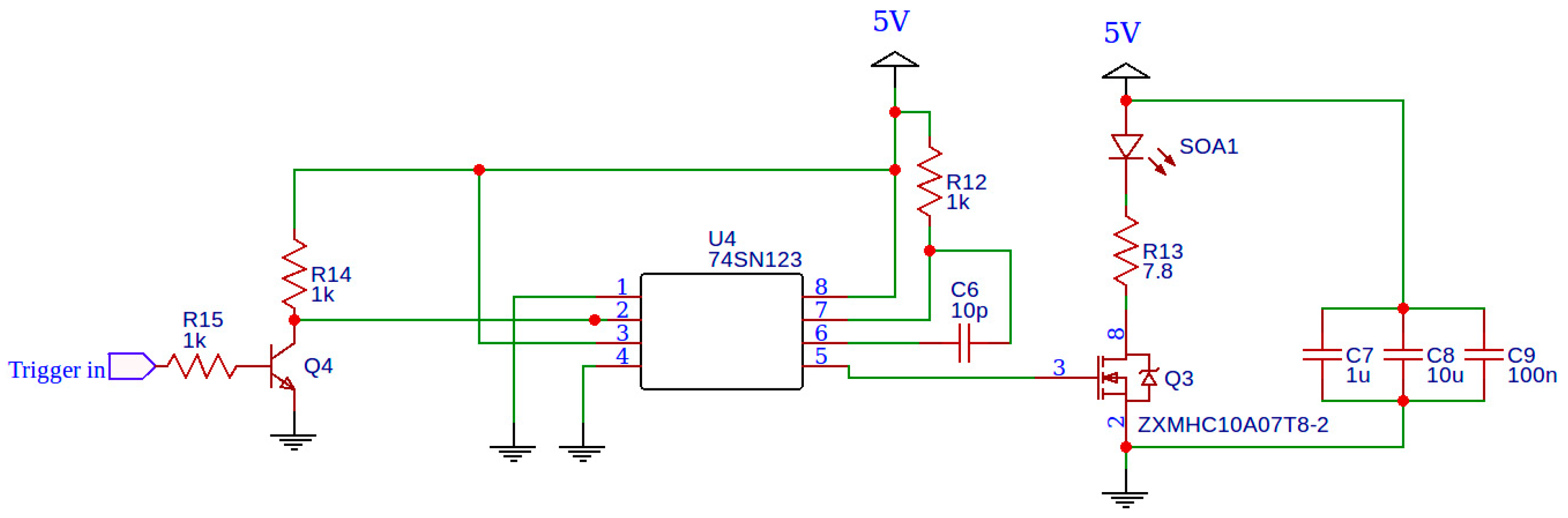
The last critical electronic element is the trigger, timer, and high current pulse generation group. This group is dedicated to the generation of the 500 mA pulses of current that drive the SOA (Thorlabs 1013SXS SM fiber) as a shutter. The system can use any SOA capable of fast switching, working in saturation and capable of managing powers on the order of tens of mW. Some SOAs require a negative bias to block the light completely during the off-state. Although such a negative bias should be as high as possible to assure maximum absorption, in practice any voltage well below the breakdown voltage (VB) of the SOA will work. Having a sufficiently “dark” off-state is a priority for this system since the EDFA that follows amplifies any small amount of light exiting the SOA at a relatively high level.
The trigger circuit (
Figure 4) uses as a trigger signal the internally generated signal by the ASG, which provides a squared signal with an arbitrary frequency that ranges between −2 and +2 V. Since the timer
U4 (74SN123) manages trigger pulses of 0–5 V, a logical inverter (
Q4), used as a level translator, is introduced between
U4 and the ASG. Therefore, the ADC digitizer is set to trigger the measurement on the falling edge of the ASG signal due to the logical inversion added by
Q4. We avoid using a second inverter in order to not increase the delay between the ADC trigger and the SOA trigger, which leads to a few additional useless samples before backscattering begins, and to reduce complexity.
6. Spatial Resolution
Spatial resolution is limited by three factors—quantization sample frequency, laser pulse duration and global system bandwidth (when the laser pulse bandwidth is greater than the system bandwidth, which is the case here). We proceed to calculate the spatial resolution arising from each limiting factor.
Regarding the quantization sample frequency, the length that the ADC digitizer can resolve,
Lq, depends on the length of the fiber that generates backscattered light between two sampling times:
where
fq is the sampling rate of the digitizer. Assuming
, Equation (7) can be simplified as:
where
fq is expressed in Giga samples/s. Since real digitizers are not noise-free, it is safe to define the minimum resolvable distance,
RS, as:
which is simplified as:
The ADC digitizer employed here allows for a maximum sampling rate of 1 GS/s, which gives an ideal spatial resolution due to quantization, RS = 30 cm. As will be shown later, this value is heavily limited by the bandwidth of the digitizer. Such a high sampling rate is useful for increasing the amplitude resolution through the down-sampling average, but when it is not necessary, the actual sampling rate should be set to no more than 2–3 times the digitizer bandwidth (according to the Nyquist theorem), making the digitizer bandwidth the limiting factor of the resolution.
Regarding the laser pulse duration, we consider a laser pulse with a time duration
τp, the spatial width of which in the fiber,
wp, is:
We consider the optical fiber lies along the x-axis in a coordinate system (x = 0 the fiber beginning and x =
L the fiber end) and a random point at x =
b on the fiber. The front edge of the laser pulse, introduced in the fiber at
t = 0, reaches the point
b at
t1 =
b/v and generates backscattered light. This backscattered light arrives at the detector (located at x = 0) at
td1 = 2
b/v. At this time, the detector also receives backscattered light, generated by the rest of the pulse width at times later than
t1 from fiber points before x =
b, which reaches the detector at
td1 because it has a shorter distance to travel. For example, the trailing edge of the pulse is located at x =
b –
wp at
t1 =
b/v. Slightly later, this trailing edge travels a distance
d =
wp/2 and reaches the location x =
b −
wp/2. This takes place at
t2 =
t1 +
wp/2v. At this point, backscattered light is generated, which reaches the detector at
td2 =
t2 + (
b −
wp/2)/v = 2
b/v =
td1. Actually, after the front edge of the pulse reaches the point x =
b, all the intermediate components of the pulse, between the front and the trailing edges, also generate backscattered light at fiber points between x =
b −
wp/2 and x =
b, which reach the detector at
td1. Therefore, at a given time, the detector receives backscattered signal not only by a single point in the fiber but instead by a fiber length
lp =
wp/2. Therefore, taking into account Equation (11), the spatial resolution due to the pulse duration is:
Assuming,
,
For a 50-ns laser pulse, this leads to a spatial resolution Rp 5 m.
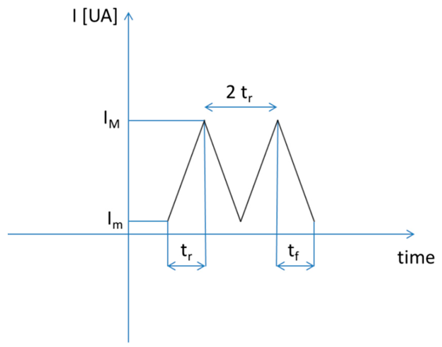
The resolution due to the global system bandwidth,
RBW, can be directly calculated with the assumption of an electronic system with symmetric rise (
tr) and fall (
tf) times, as shown in
Figure 6.
According to
Figure 6, the time between two events at the minimum resolvable distance is twice the rise/fall time. It is well known that in analog systems the rise/fall time is related to the bandwidth,
BW, by:
As light travels in the optical fiber with a velocity
c/neff and generates the backscattered signal, the relation between detection time,
t, and generation position in the fiber,
l, is:
therefore, if we consider
t = 2
tr the time corresponding to the length equal to the resolution due to the bandwidth (with
l =
RBW), we have:
which gives:
simplified as:
combining Equation (18) with Equation (14),
RBW becomes:
Since the bandwidth of the system is 200 MHz, as we mentioned in
Section 2, the theoretical spatial resolution,
RBW, is 33 cm.
The final resolution of the system is the maximum of the three resolutions calculated above, which is the 5-m resolution due to the laser pulse duration. Therefore, the system resolution can be reduced to sub-meter values for laser pulse durations less than 10 ns. However, a pulse duration decrease (equivalently, a decrease of the pulse width in the fiber,
wp) leads to a system sensitivity and S/N ratio decrease, since [
31]:
Even though the 5-m resolution could be rather low for some SHM applications, there are many SHM applications for which this resolution is appropriate. Moreover, the resolution plays a minor role in applications where it not necessary to spatially resolve different events, but it is important to precisely locate and detect a single event.
7. System Demonstration
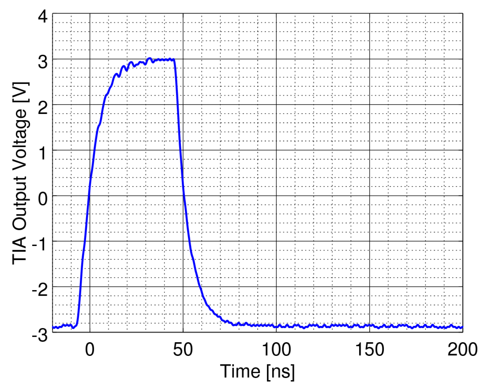
By design, the optical pulse generator provides 50 ns pulses with rise/fall times below 2 ns when charged on a resistive load.
Figure 7 shows the retrieved laser pulse output by the SOA directly to the TIA amplifier and digitized by the ADC using an attenuator to limit the power arriving at the photodetector. The pulse shows rise and fall times of ~13 ns. These values can be considered as a metric of the final system performance, as the rise and fall times are directly connected to system total bandwidth, set by the interaction between the SOA, pulse generator, TIA amplifier, digitizer and the electric connections between these elements.
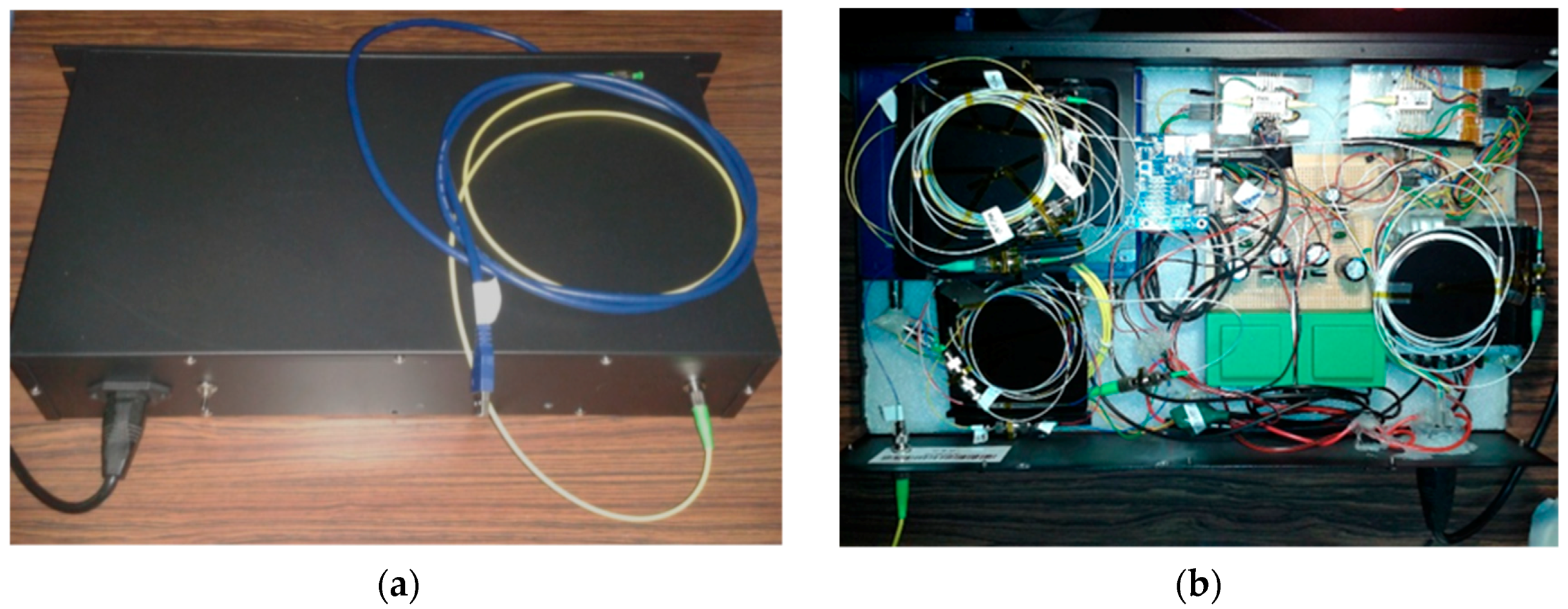
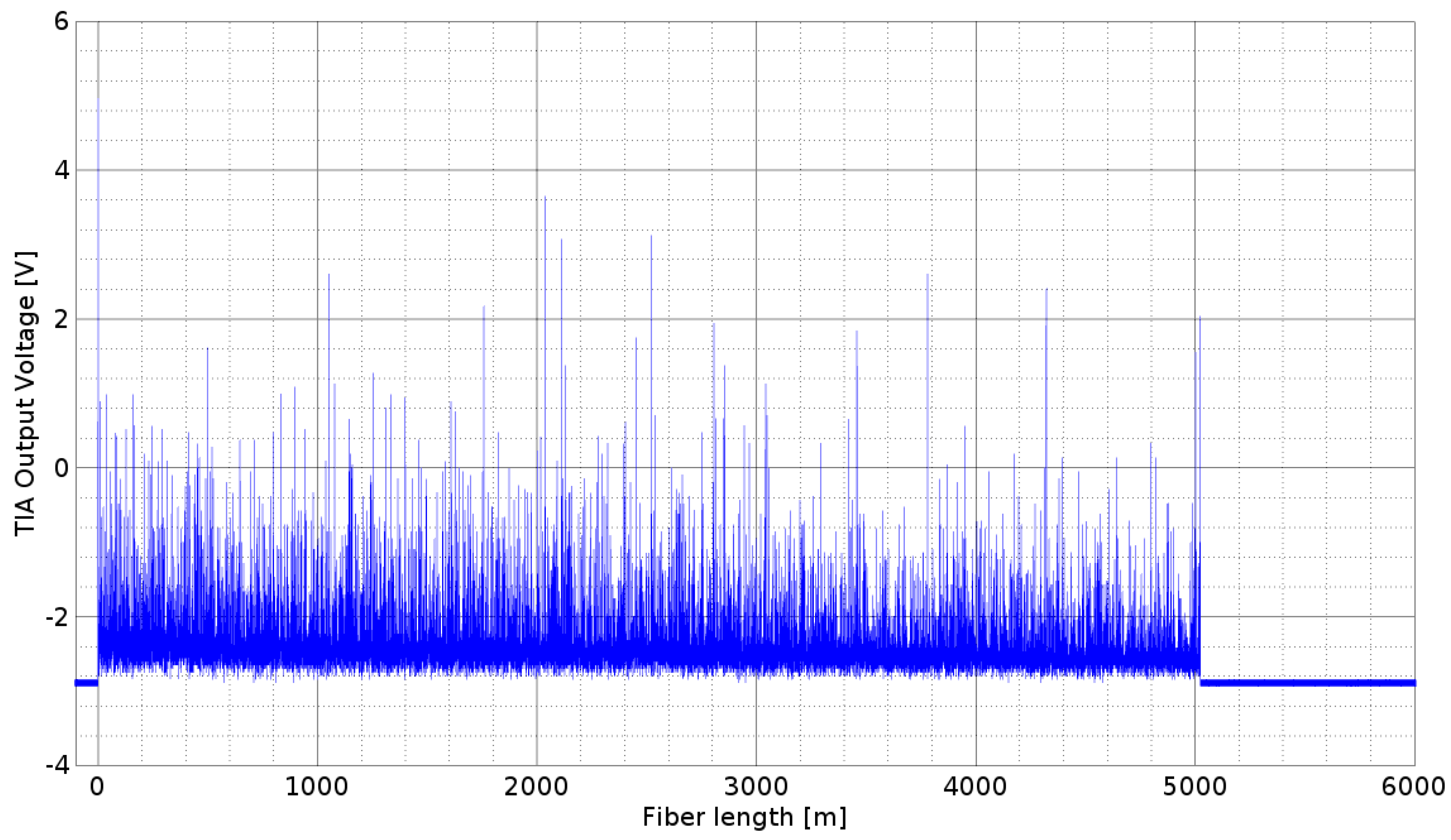
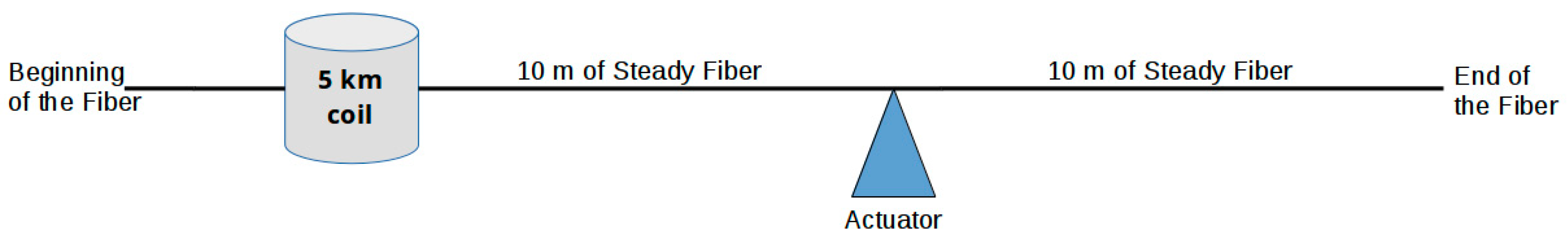
Figure 8 presents the backscattered signal collected by the TIA amplifier for a 5-km long optical fiber, connected with a 20 m lead fiber of the same type, as shown in
Figure 9. According to what is shown in
Figure 8, the noise baseline is about ±47.5 mV over a scale of −5 V to +5 V; since the vertical resolution is about 47.5 mV, the noise is about 1.6 bit. This noise value is similar to that of the digitizer with no input, but it has a higher spectral content when the TIA is connected to the digitizer, demonstrating that the TIA contributes to the system noise, although not enough to produce a significant effect since the digital magnitude remains below 1.6 bit.
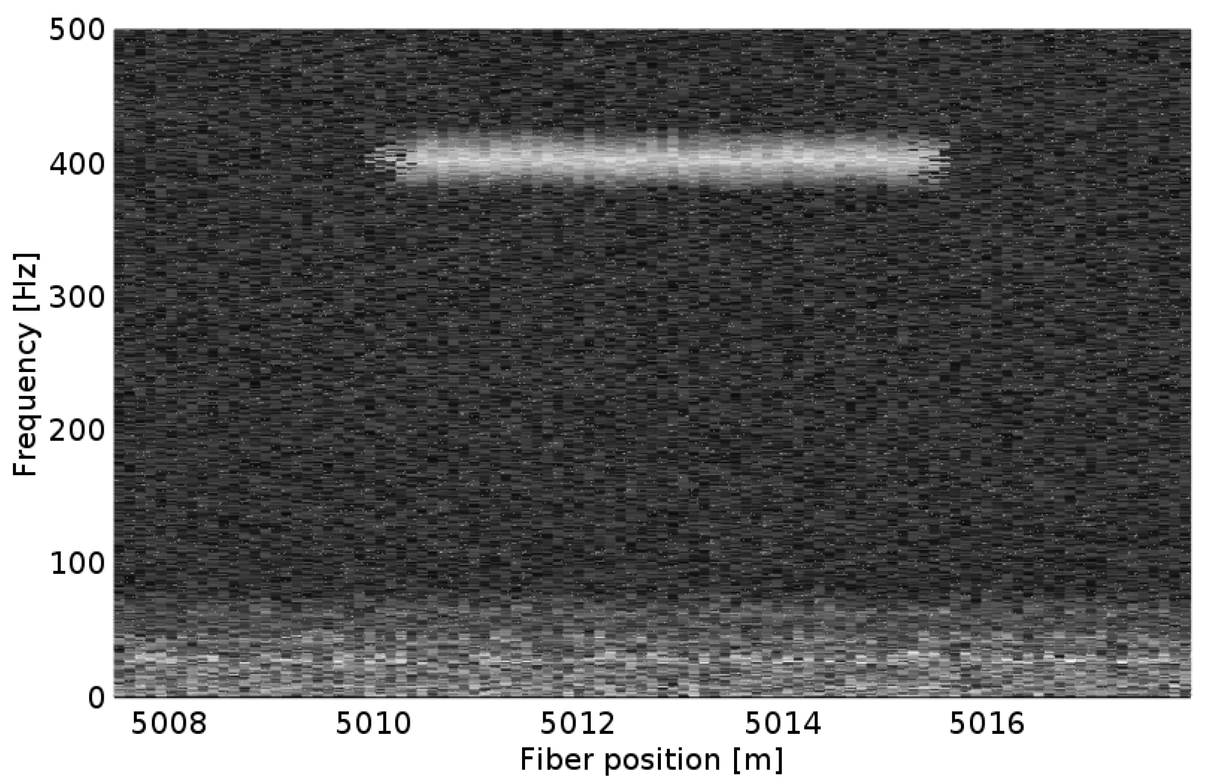
The 20 m of lead fiber was used as depicted in
Figure 9 to allow monitoring of the system response to a specific harmonic of 400 Hz. An actuator introduced a harmonic tone in the middle of the lead fiber (corresponding to fiber length ~5013 m in
Figure 8), while the rest of the fiber is kept steady.
The magnitude of the harmonic tone was set to the minimum detectable value to minimize the portion of the fiber under the effect of the vibration. With a 10 kHz track interrogation rate and a 10x averaging factor, the actual track interrogation rate is 1 kHz. This interrogation rate allows the capturing of signals up to 500 Hz. This test allowed the determination of the spatial resolution of the system due to the laser pulse duration, Rp (since the limiting factor of the spatial resolution is the pulse duration).
As shown in
Figure 10, the spatial resolution of the system is ~6 m, close to the calculated value of 5 m. Indeed, the 400-Hz tone is applied at
L = 5013 m, and the system detects it at
L = 5010–5016 m.


