3.2. Signal (Non)linearity
Calorimeters may be non-linear for a variety of reasons. Intercalibration of longitudinal sections, signal saturation and the energy dependence of the em shower fraction (in hadron showers) are the most common causes. Many calorimeters are non-linear, even though their owners sometimes pretend otherwise.
A common misconception is that a calorimeter is linear if the average signals plotted versus the deposited energy can be described with a straight line. This is not what is meant by a linear calorimeter. The straight line has to extrapolate through the origin of the plot. Signal linearity means that the average calorimeter signal is proportional to the deposited energy, i.e., the response is constant.
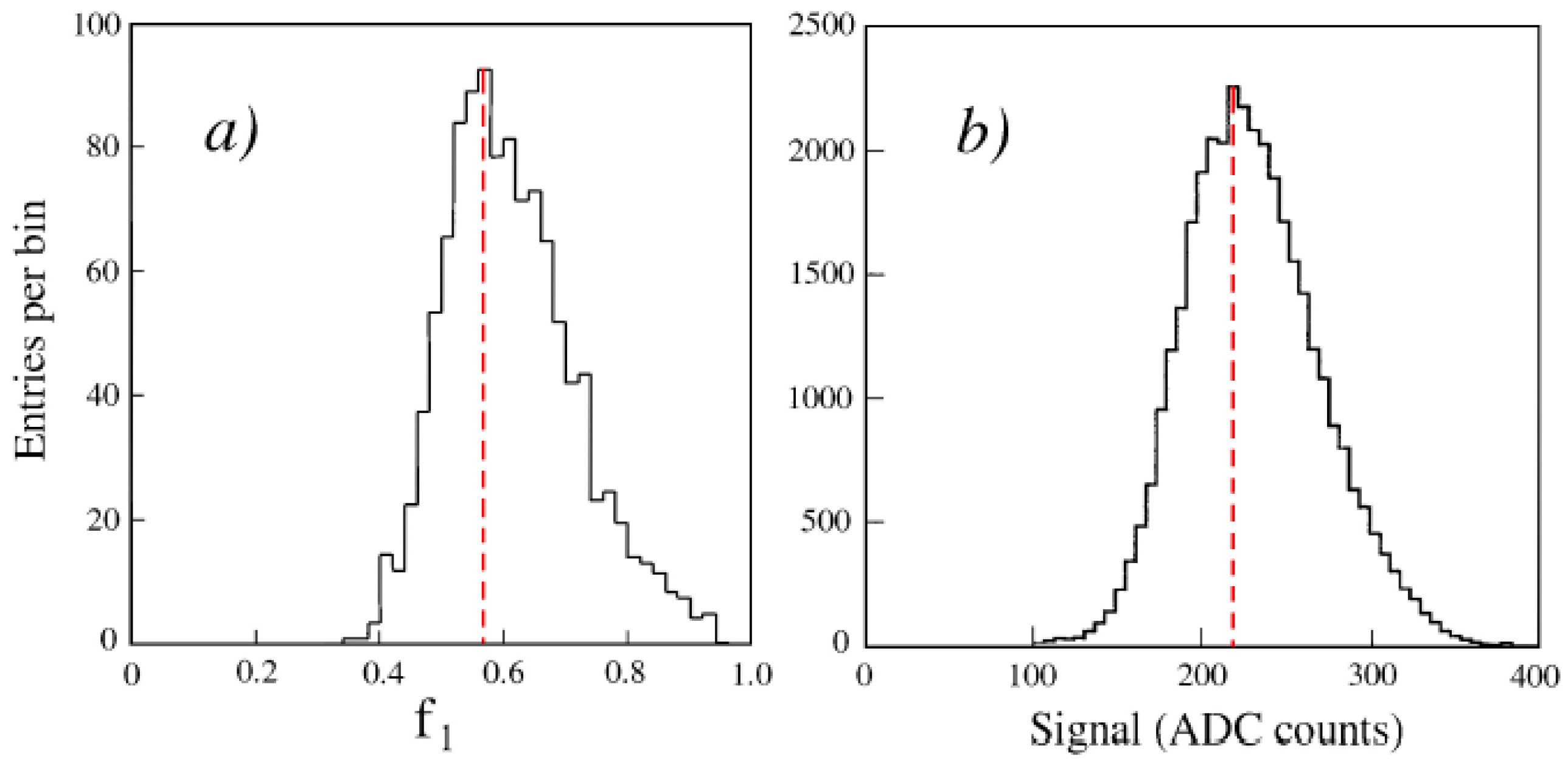
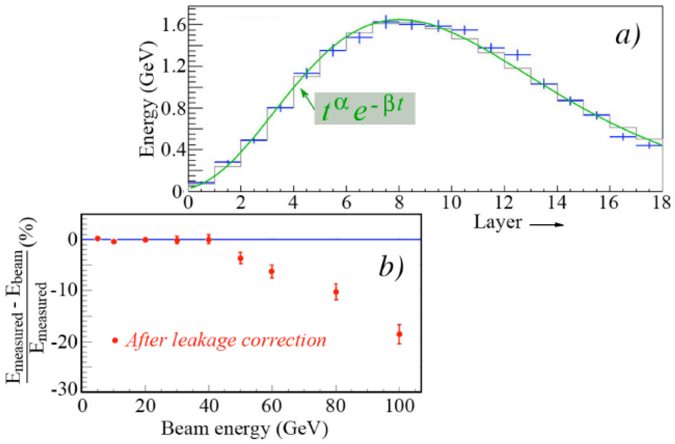
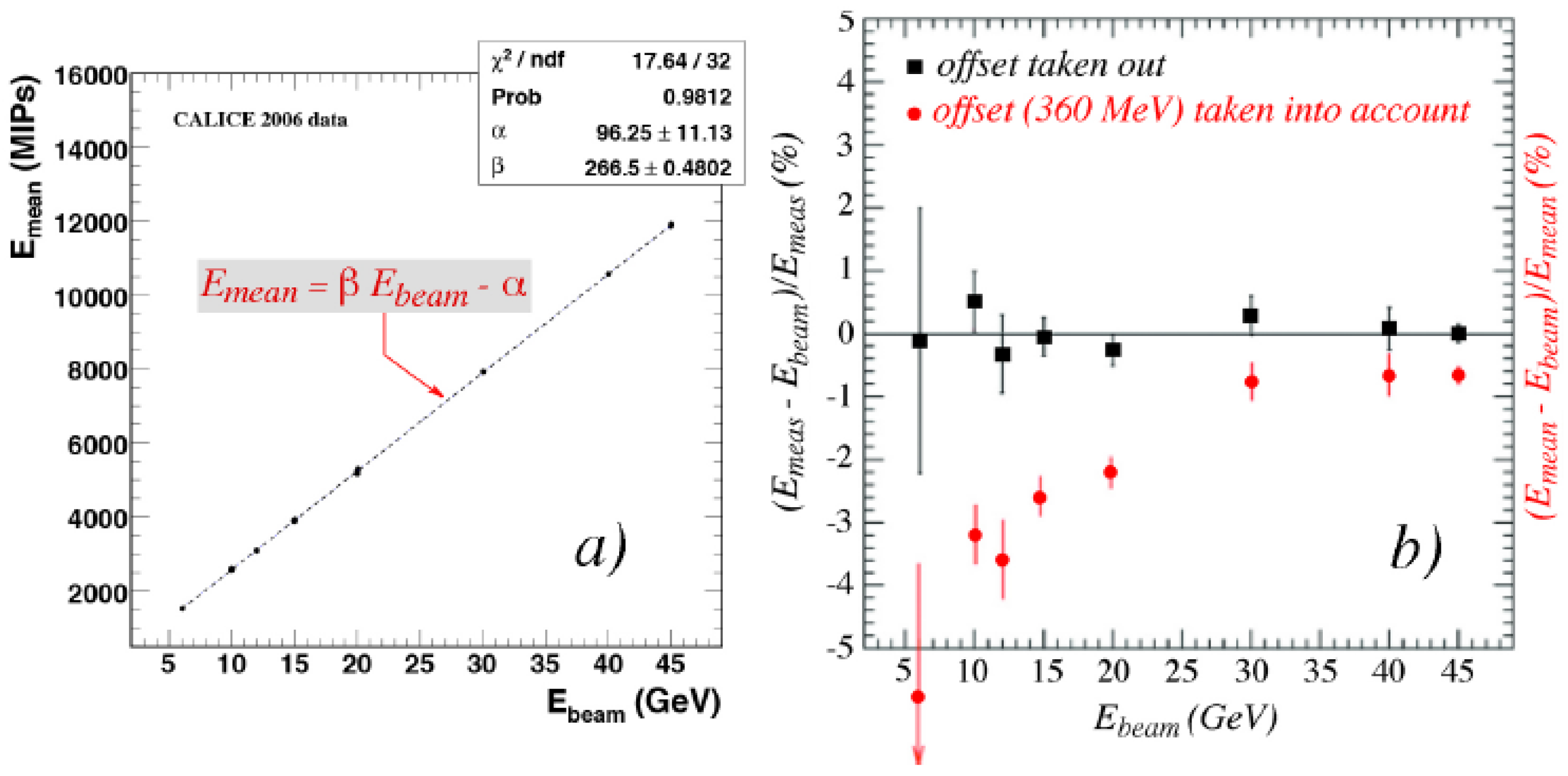
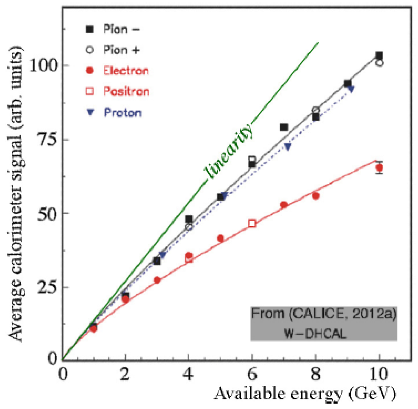
Figure 4 illustrates this issue. The experimental data were obtained with a W/Si em calorimeter built by CALICE [
18]. The authors fit the measured signals with the following expression:
Then, they define
and plot
as a function of the beam energy. The result is represented by the (black) squares in
Figure 4b. They conclude that “the calorimeter is linear to within approximately 1%”. This is highly misleading. When the calorimeter signals they actually measured are used to check the linearity, i.e., when
is plotted as a function of the beam energy, the results, represented by the (red) full circles in
Figure 4b, look quite different. We conclude from these results that the authors measured a signal non-linearity of 5% over one decade in energy.
3.2.1. Non-Linearity Resulting from Signal Saturation
Whereas the non-linearity discussed in the previous subsection is probably the result of the intercalibration of the numerous longitudinal segments of this PFA calorimeter,
Figure 5 shows non-linearity with a different origin. It concerns data obtained with a digital hadron calorimeter built by CALICE [
14]. This calorimeter contains 500,000 readout cells (
cm
2 RPCs), which produce “digital” signals (“yes” or “no”) in response to charged particles. However, this type of cell produces the same signal, regardless whether it is caused by 1, 3 or 29 shower particles. This leads to signal non-linearity, especially in em showers. Since the lateral shower profile is independent of the energy of the showering particle, and the longitudinal shower profile only varies logarithmically with that energy, the density of shower particles in the region where the energy is deposited increases almost proportionally with the shower energy, signal non-linearity is
inevitable. The same is true for hadron showers, albeit that the shower particle density is smaller in that case, and the non-linearity effects correspondingly less pronounced.
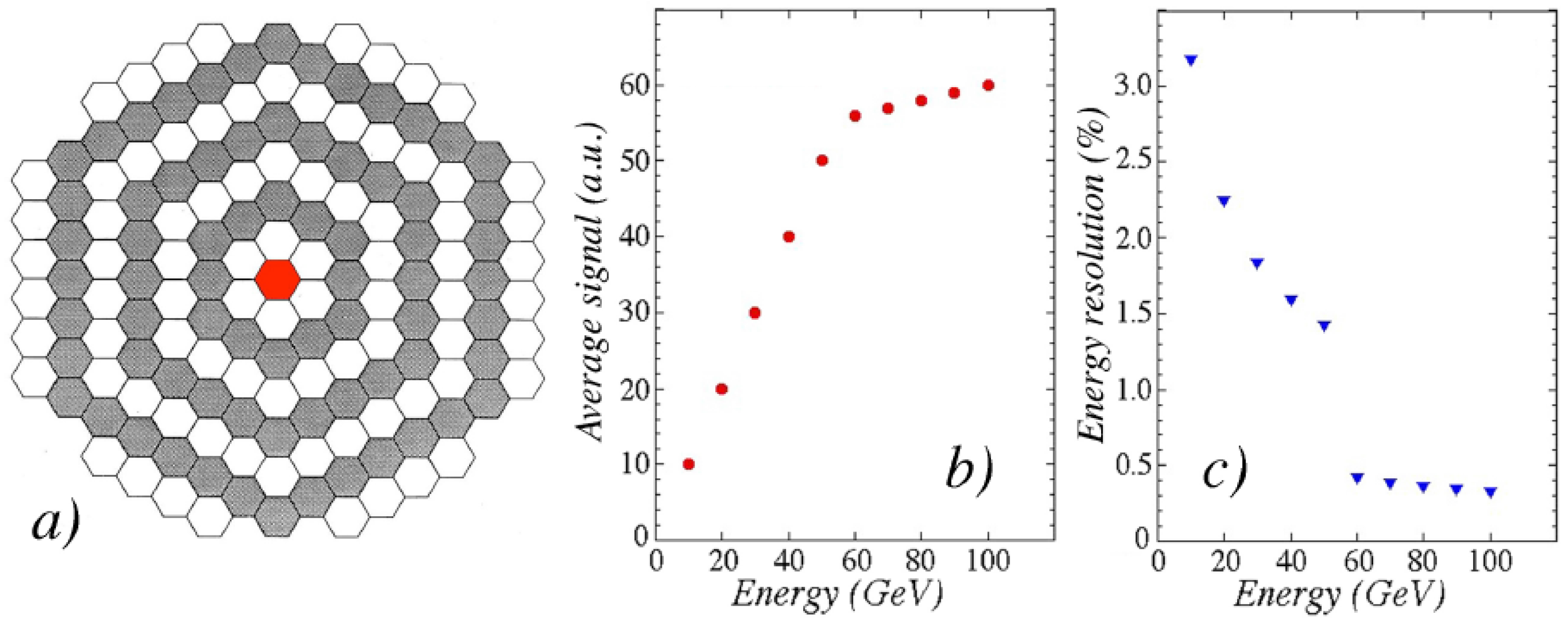
We use data from one of our own experiments to illustrate the effects of signal saturation. The SPACAL calorimeter (
Figure 6a) consisted of 155 hexagonal towers. Each of these towers was calibrated by sending a beam of 40 GeV electrons into its geometric center. Typically, 95% of the shower energy was deposited in that tower, and the remaining 5% was shared among the six neighbors. The high-voltage settings were chosen such that the maximum energy deposited in each tower during the envisaged beam tests would be well within the dynamic range of that tower. For most of the towers (except the central septet), the dynamic range was chosen to be 60 GeV.
When we did an energy scan with electrons in one of these non-central towers, the results shown in
Figure 6b and c were obtained. Up to 60 GeV, the average calorimeter signal increased proportionally with the beam energy, but above 60 GeV, a non-linearity became immediately apparent (
Figure 6b). The signal in the targeted tower had reached its maximum value, and would from that point onward produce the same value for every event. Any increase in the total signal was due to the tails of the shower, which developed in the neighboring towers. A similar trend occurred for the energy resolution (
Figure 6c). Beyond 60 GeV, the energy resolution suddenly improved dramatically. Again, this was a result of the fact that the signal in the targeted tower was the same for all events at these higher energies. The energy resolution was thus completely determined by event-to-event fluctuations in the energy deposited in the neighboring towers by the shower tails.
A similar situation occurred in the CALICE calorimeter of which the results are shown in
Figure 5. And since also in this calorimeter an important source of fluctuations is suppressed, the energy resolution measured with it is meaningless. We should emphasize that the described effects may in practice be less obvious, especially in more complicated setups and for complex events.
3.2.2. Non-Linearity for Hadron Detection
Calorimeters intended for the detection of hadron showers are typically intrinsically non-linear, as a result of the fact that the average em shower fraction depends on the energy of the showering particle. Non-compensating calorimeters respond differently to the em and non-em shower components (), and the overall calorimeter response reflects the fact that the energy sharing between these shower components is energy dependent. These signal non-linearities for hadron detection are thus the result of the physics of the shower development process, they do not depend on peculiarities of the calorimeter signals, as in the examples described in the previous subsection. For that reason, hadronic signal non-linearity does in general not preclude an (on average) correct measurement of the energy of the showering particle on the basis of the observed signals. This is not necessarily true for all the non-linearities that may affect electromagnetic shower detection, such as the ones discussed in the next subsection.
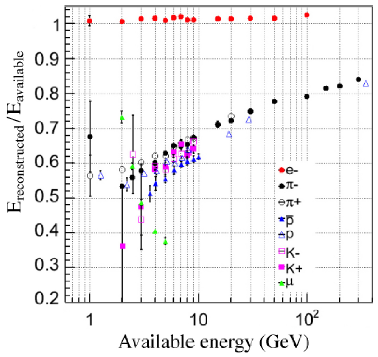
A (on average) correct measurement of hadronic energy deposits is possible, provided that the em energy scale has been determined in the same way for all longitudinal calorimeter segments. In that case the hadronic response can be determined with hadron beams of different energy, using the em energy scale. An example is shown in
Figure 7. The correct hadron energy is then found by multiplying the measured energy with the inverse of the calorimeter response for that energy. The figure shows slightly different responses for different types of hadrons, but in CMS this is a secondary effect compared to the large dependence of the response on the starting point of the showers [
19].
3.2.3. Signal Non-Linearity as a Result of Miscalibration
One of the most common reasons for signal non-linearity is the method chosen to intercalibrate the various longitudinal sections of a longitudinally segmented calorimeter. This is illustrated with the example of the HELIOS calorimeter [
20], discussed below. This calorimeter consisted of two longitudinal segments, with depths of
and 4
, respectively (
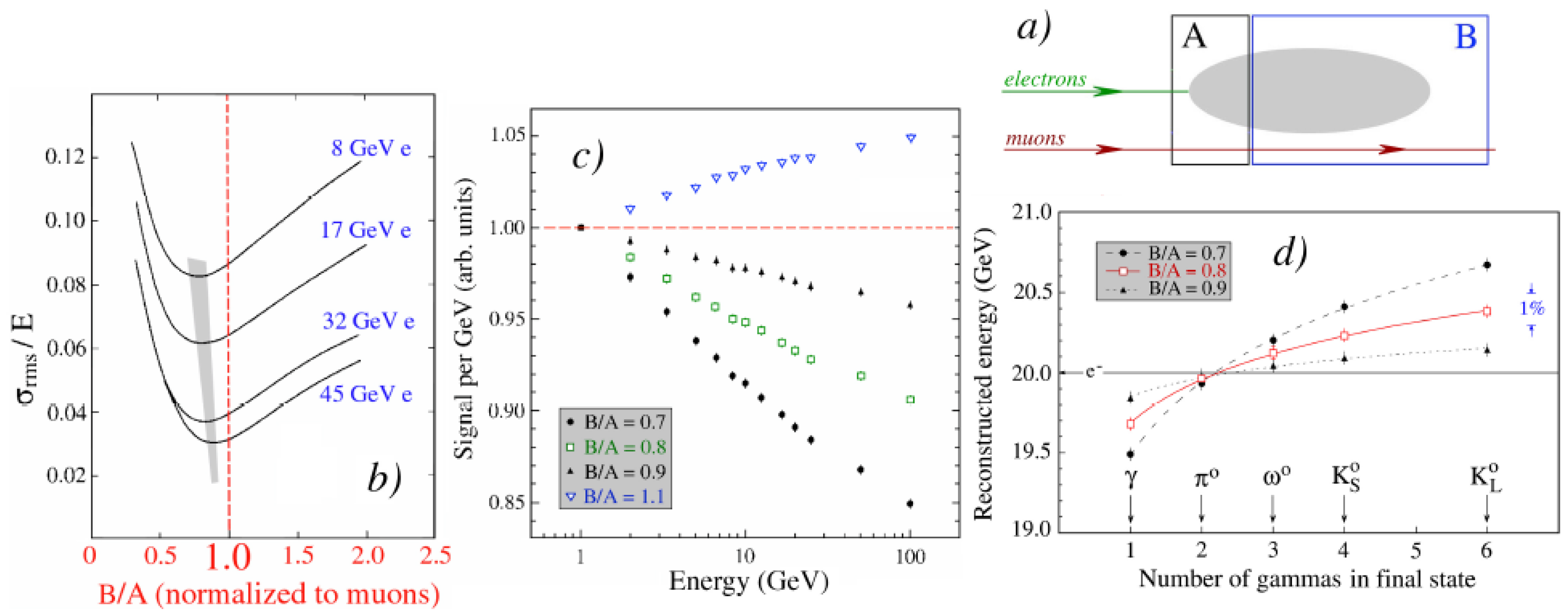
Figure 8a). Electrons developing in this structure deposited comparable amounts of energy in each section, but the precise energy sharing depended on the energy of the showering particle. The intercalibration of the signals from the two sections was performed by minimizing the width of the total signal distribution.
Figure 8b shows how this width depended on the choice of the ratio of the calibration constants for the signals from both sections,
. The optimum value turned out to be different from the value for muons. The latter could simply be calculated from the composition of the two sections.
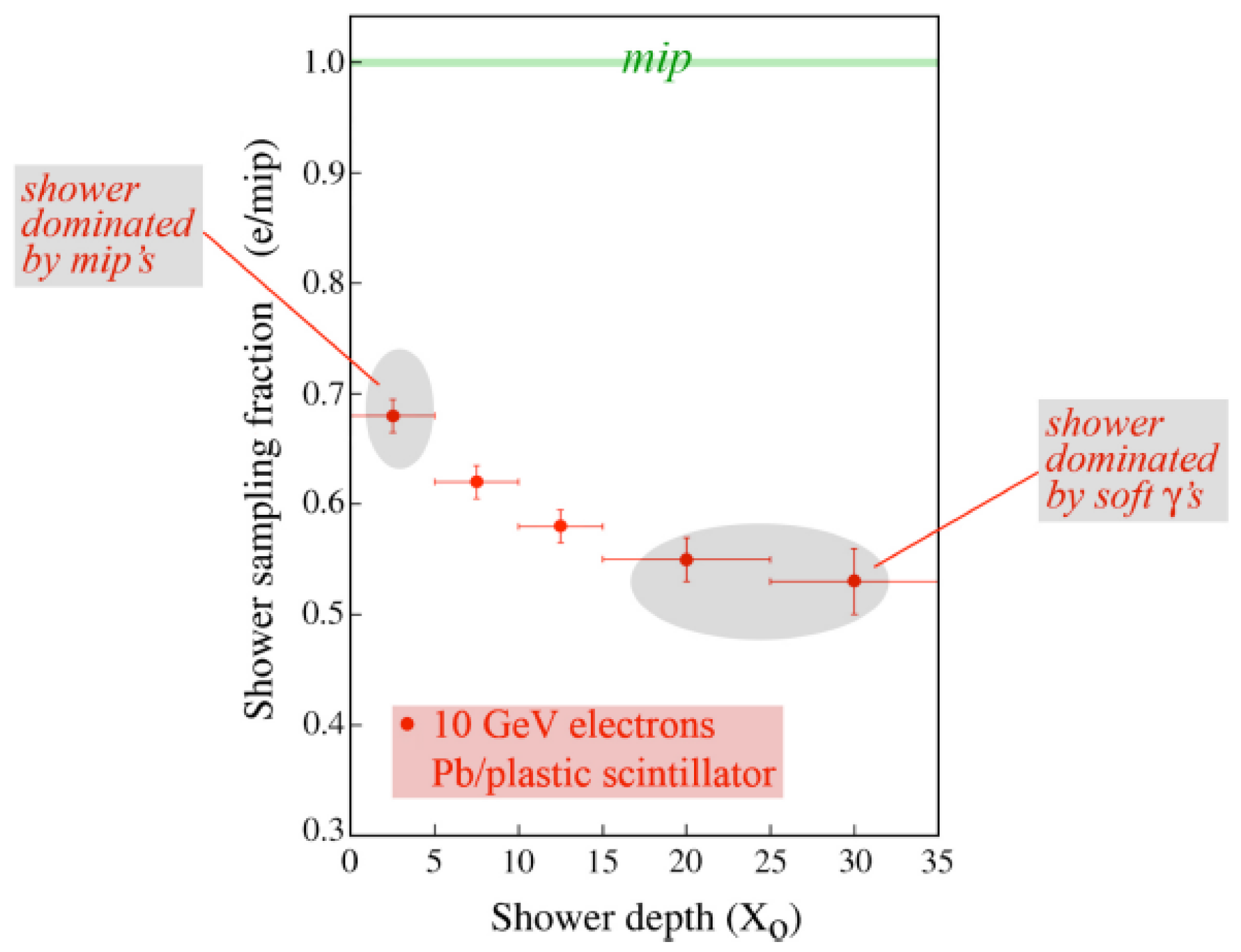
If we take
for muons, then the optimal value for electrons was around 0.6–0.9, depending on the energy. This can be understood from the fact that the sampling fraction decreased as the shower developed (
Figure 1). Since the sampling fraction in the first section was larger, a smaller total width was obtained when signals from that section were attributed a relatively larger weight, hence the optimal value
. Now, if the electron energy increases, a larger fraction of that energy is deposited in the second calorimeter section. And since the signals from that section are given a relatively small weight, the result is a total signal that is smaller than if the signals from both sections had been given the same weights as mips (
). In other words, the calorimeter
response (i.e., the average signal per GeV) decreases.
A calibration procedure in which the width of the total signal distribution of showers that develop in several different calorimeter segments is minimized thus leads inevitably to a non-linear response. Now one might argue that there is in principle no reason why a calorimeter that is non-linear for electromagnetic shower detection, although somewhat inconvenient, should be unacceptable. After all, all non-compensating calorimeters are intrinsically non-linear for hadron and jet detection and one uses those too, in many experiments.
Any type of non-linearity could in principle be dealt with by means of a polynomial relationship between the signals
S and the corresponding energy
E:
and the fact that other constants than
have a non-zero value might be a small price to pay for improving energy resolution.
This line of reasoning is, however, crucially flawed [
21]. The non-linearity introduced by this weighting scheme implies by definition that a high-energy
, decaying into two unresolved
s produces, on average, a larger signal in this calorimeter than an electron, or one photon, of the same energy. An
resonance decaying into three unresolved
s produces an even larger signal, and an energetic
decaying into
, or even
tops them all (
Figure 8d). By introducing a signal non-linearity, the calorimeter response is made dependent on such differences. And since, in practice, the calorimeter information does not always allow one to tell whether the signal was caused by one, two, three or even more
s, the systematic differences in the average calorimeter response for those cases are an integral part of the energy resolution. Interpreting the width of the signal distribution measured for single electrons from a test beam as the em energy resolution is thus incorrect.
The approach chosen in this case (minimization of the width of the total signal distribution) is only one of several different methods described in the literature for intercalibrating the different sections of a longitudinally segmented calorimeter. Other methods aim to achieve
Correct energy reconstruction of pions penetrating the electromagnetic compartment without starting a shower, or
Hadronic signal linearity, or
Independence of hadron response on starting point shower, or
Equal response to electrons and pions.
Each of these approaches introduces specific additional problems [
22]. Intercalibrating the different sections of a longitudinally segmented calorimeter system is in practice one of the most daunting tasks when commissioning a detector, and it is fundamentally impossible to achieve a result in which the signals measured in the different sections can be correctly translated into deposited energy. This is even true for compensating calorimeters. The combination of the energy dependence of the shower profiles, combined with the depth dependence of the sampling fraction are responsible for this problem.
The best way to intercalibrate the different sections of a longitudinally segmented calorimeter system is by using the same particles for all individual sections. If these particles develop showers, then they can only be used to calibrate sections in which these showers are completely contained. Only in this way is the relationship between the deposited shower energy (in GeV) and the charge (in picoCoulombs) generated as a result established unambiguously. We have referred to this as the
method. The use of a beam of muons to intercalibrate the eighteen segments of the AMS-02 electromagnetic calorimeter (
Figure 2) definitely qualifies as a viable method in this respect. The mistake made in that case did not concern the calibration method itself, but the interpretation of the results.
3.3. Energy Resolution
A common mistake with regards to energy resolution has to do with its very definition. The energy resolution is the precision with which the energy of an unknown object can be determined from the signals it produces in the calorimeter. Typically, this resolution is determined as the relative width of the signal distribution measured for a beam of mono-energetic particles from an accelerator. However, this is only correct if the average value of that measured signal distribution corresponds indeed to the correct energy of these particles. Response non-linearities tend to invalidate that assumption, as illustrated by the example shown in
Figure 8d.
Often, the measured signal distributions exhibit non-Gaussian tails. In that case, one should quote the
value as the energy resolution. However, some authors use another variable, in order to make the results less dependent on the tails of the signal distributions they measure, and thus look better. This variable, called
, is defined as the root-mean-square of the energies located in the smallest range of reconstructed energies which contains 90% of the total event sample. For the record, it should be pointed out that for a perfectly Gaussian distribution, this variable gives a 21% smaller value than the true
(i.e.,
). Of course, one is free to define variables as one likes. However, one should then not use the term “energy resolution” for the results obtained in this way, and compare results obtained in terms of
with genuine energy resolutions from calorimeters with Gaussian response functions [
23]. This misleading practice is generally followed by the proponents of PFA.
Another widespread misconception concerns the way in which the energy resolution of a calorimeter is quoted. Frequently, the relative energy resolution () of a particular calorimeter is expressed as . However, this is rarely a correct description of reality, since in practice other factors, which are not governed by Poisson statistics, contribute to the energy resolution, and such factors often dominate the performance, especially at the low and high ends of the energy spectrum for which the detector is intended.
As an example,
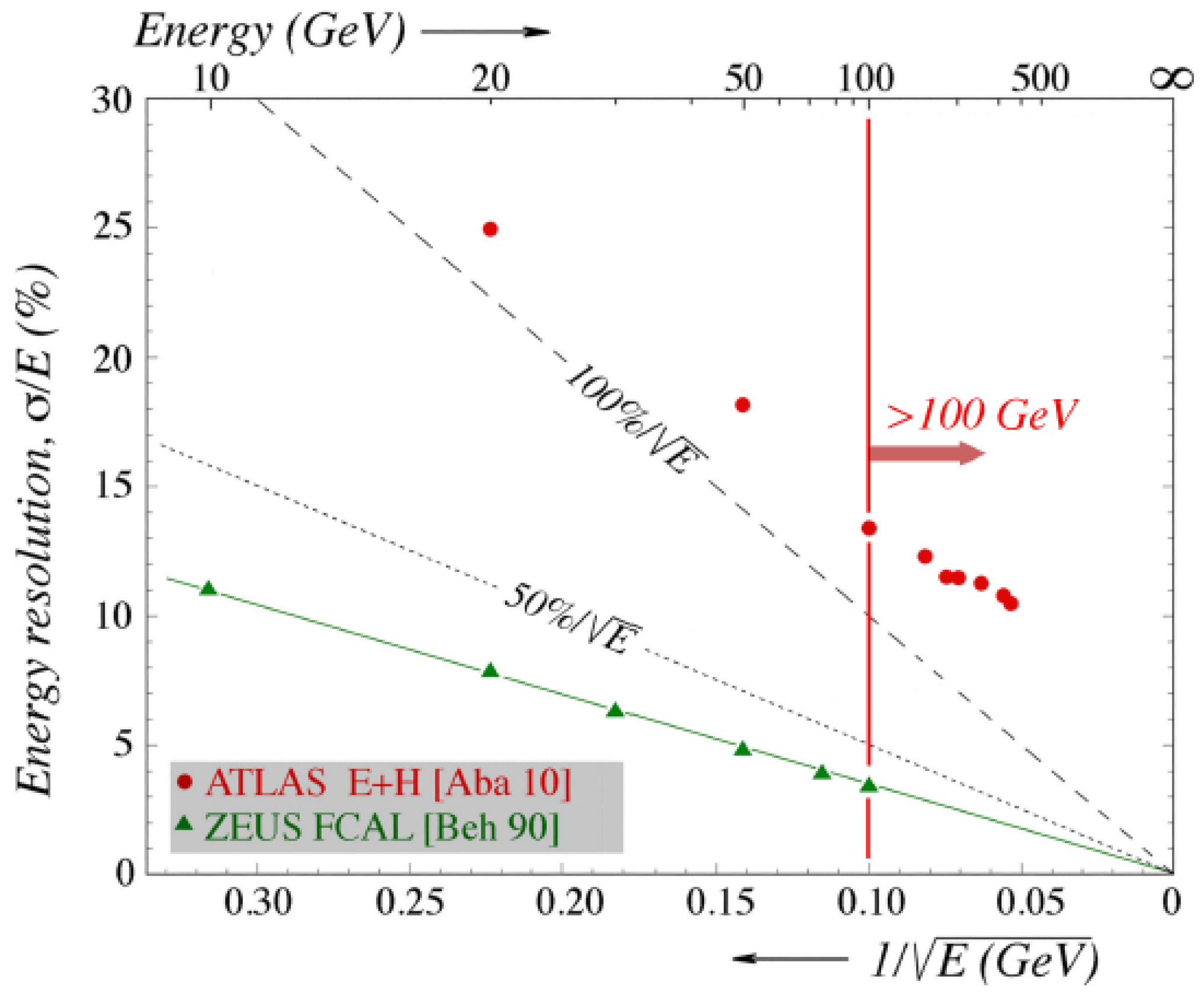
Figure 9 shows the hadronic energy resolutions of the ZEUS and the ATLAS calorimeters. The experimental data points are plotted on a scale that is linear in
and runs from right to left. Scaling with
implies that the data points should be located on a straight line through the bottom right corner in this plot. This is indeed the case for the compensating ZEUS calorimeter, for which the resolution is quoted as
. However, the resolution of ATLAS does not at all scale with
. As a matter of fact, the data points are at all energies located well above the
line in this plot, and for energies larger than 100 GeV, the resolution is more than a factor of four worse than for ZEUS. Yet, in talks about ATLAS, the hadronic energy resolution is often quoted as
.
Another mistake that is not uncommon concerns the extrapolation of measurement results far beyond their region of validity, We mention two examples.
The HELIOS Collaboration measured a resolution
for 3.2 TeV
16O ions [
20], and the WA80 Collaboration, which also operated a uranium/scintillator calorimeter, found a resolution of 1.7% for 6.4 TeV
32S ions [
26]. One should realize, however, that in these cases a convolution of either 16 or 32 independent 200 GeV nucleon showers was measured. Hence, strictly speaking, these results only say something about the precision of the energy measurement for a 200 GeV nucleon shower. If sixteen signals from such showers are convolved, then the resulting signal has a resolution
that is four (=
) times smaller than the resolution for the individual signals from 200 GeV nucleons. In other words, if the resolution for 200 GeV protons (or neutrons) was 7.6%, then a resolution of 1.9% should be expected for
16O ions with an energy of 3.2 TeV. The measured resolution for heavy ions at multi-TeV energies is thus by no means indicative for the resolution that may be expected for the detection of single hadrons or jets carrying such energies.
A similar statement should be made concerning the “determination” of the energy resolution for high-energy electromagnetic shower detection in liquid xenon, based on convolving the signals from large numbers of low-energy electrons (100 keV) recorded in a small cell [
27]. Also in this case, the measurements only revealed something about the energy resolution for the detection of these low-energy electrons. In a high-energy em shower, a variety of new effects, absent or negligible in the case of these electrons, affect the signals and their fluctuations. As an example of such effects, we mention the fact that the (174 nm) shower light is produced in a large detector volume. Light attenuation, e.g., through self-absorption and shower leakage, are the likely consequences of this.
These examples illustrate that, in general, measurements made for low-energy particles cannot be used to determine/predict the high-energy calorimeter performance.
Finally, we want to point out that often times a good energy resolution is only part of the requirements for obtaining the desired physics sensitivity. As an example, we mention the Higgs boson, discovered in 2012 by two experiments at the Large Hadron Collider through its decay mode
[
28,
29]. The invariant mass of a particle decaying into two
s is given by
The precision with which the mass can be measured is thus not only determined by the energy resolution, i.e., the measurement uncertainty on the energies and , but also by the relative uncertainty on the angle () between the directions of these s. A good localization of the s is thus very important to identify the parent particle. While CMS emphasized excellent energy resolution for em showers in its design of the experiment, at the expense of degraded hadronic performance, ATLAS concentrated its efforts also on the localization issue. As a result, the mass resolution for the Higgs bosons turned out to be very similar in both experiments.
3.4. Effects of Non-Compensation
Almost all calorimeters that are operating in large storage ring experiments are non-compensating. This means that the responses (i.e., the average signal per unit deposited energy) to the em and non-em components of hadron showers are not the same in these calorimeters (). The consequences of this feature are a source of several misconceptions. Often, an additional constant term in the hadronic energy resolution is considered the main, if not the only, consequence of non-compensation. This is a misconception at several levels. Not only is non-compensation the cause of a number of other serious problems, but the effect on the hadronic energy resolution is by no means independent of energy, as suggested by the concept of an additional constant term.
The incorrectness of this notion is illustrated by the fact that the hadronic energy resolution of non-compensating calorimeters is not only considerably worse compared to compensating ones at high energies, but also at low energies. The resolution of the best hadron calorimeters, such as the one used for the ZEUS experiment [
24], is ∼30%/
, i.e.,
at 10 GeV (
Figure 9). Adding a constant term of 5% (in quadrature) would increase this resolution to ∼11%. However, the energy resolution of non-compensating calorimeters is typically two to three times larger at this energy. The effects of non-compensation are thus by no means limited to high energy, where a constant term tends to dominate the contributions that are determined by Poisson fluctuations.
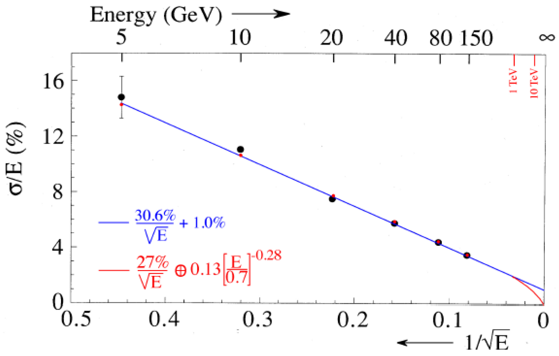
The correct way of incorporating the effects of non-compensation on the hadronic energy resolution is given by Equation (
7), and illustrated in
Figure 10.
The effects are described by an energy dependent term, added in quadrature to the scaling term that accounts for the Poisson fluctuations (
in this example). The coefficient of this non-compensation term,
in this example, is determined by the degree of non-compensation:
, and
[
30].
Figure 10 also shows that the correct description of the hadronic energy resolution yields in practice almost identical results as an expression in which a constant term (
) is added linearly to a scaling term (
). There are several examples in the literature in which such an expression is used to describe the hadronic energy resolution. However, the linear addition of two terms suggests complete correlation between the effects described by these terms, which is nonsense in this situation.
Figure 10 shows that one has to go to very high energies, beyond the reach of the current generation of available test beams, to see a significant difference between the two mentioned expressions. However, only one of these expressions (the red one) is correct, and indicates that the effects of non-compensation on the hadronic energy resolution are indeed energy dependent.
However, a hadronic energy resolution that deviates from scaling is not the only consequence of non-compensation. Among the other effects, we mention
Hadronic signal non-linearity (see
Section 2.2.2). This is a result of the fact that the average em fraction of hadron showers,
, increases with energy.
Non-Gaussian response functions. This is a consequence of the fact that the distribution of
is not Gaussian, but asymmetric, favoring large values (
Figure 11).
This may cause problems, such as trigger biases. For example, if one uses the calorimeter signals to select events with a minimum (missing) transverse energy from a steeply falling distribution, then the event sample is likely to be strongly dominated by events in which the actual value of this energy was smaller than the trigger level, but in which upward fluctuations pushed it beyond that level. An asymmetric response function makes it very difficult to deal with this problem in a correct way.
Different response functions for different hadrons (protons, pions, kaons) of the same energy. This is the topic of the next subsection.
3.5. Particle Dependence of the Calorimeter Response
The absorption of different types of hadrons in a calorimeter may differ in very fundamental ways, as a result of applicable conservation rules. For example, in interactions induced by a proton or neutron, conservation of baryon number has important consequences. The same is true for strangeness conservation in the absorption of kaons. This has implications for the way in which the shower develops. For example, in the first interaction of a proton, the leading particle has to be a baryon. This precludes the production of an energetic
which carries away most of the proton’s energy. Similar considerations apply in the absorption of strange particles. On the other hand, in pion-induced showers it is not at all uncommon that most of the energy carried by the incoming particle is transferred to a
. The resulting shower is in that case almost completely electromagnetic. This phenomenon is the reason for the asymmetric distributions from
Figure 11.
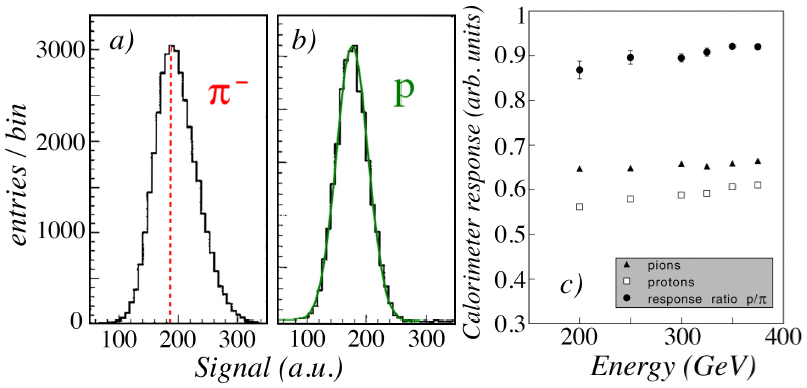
Experimental studies have confirmed these effects.
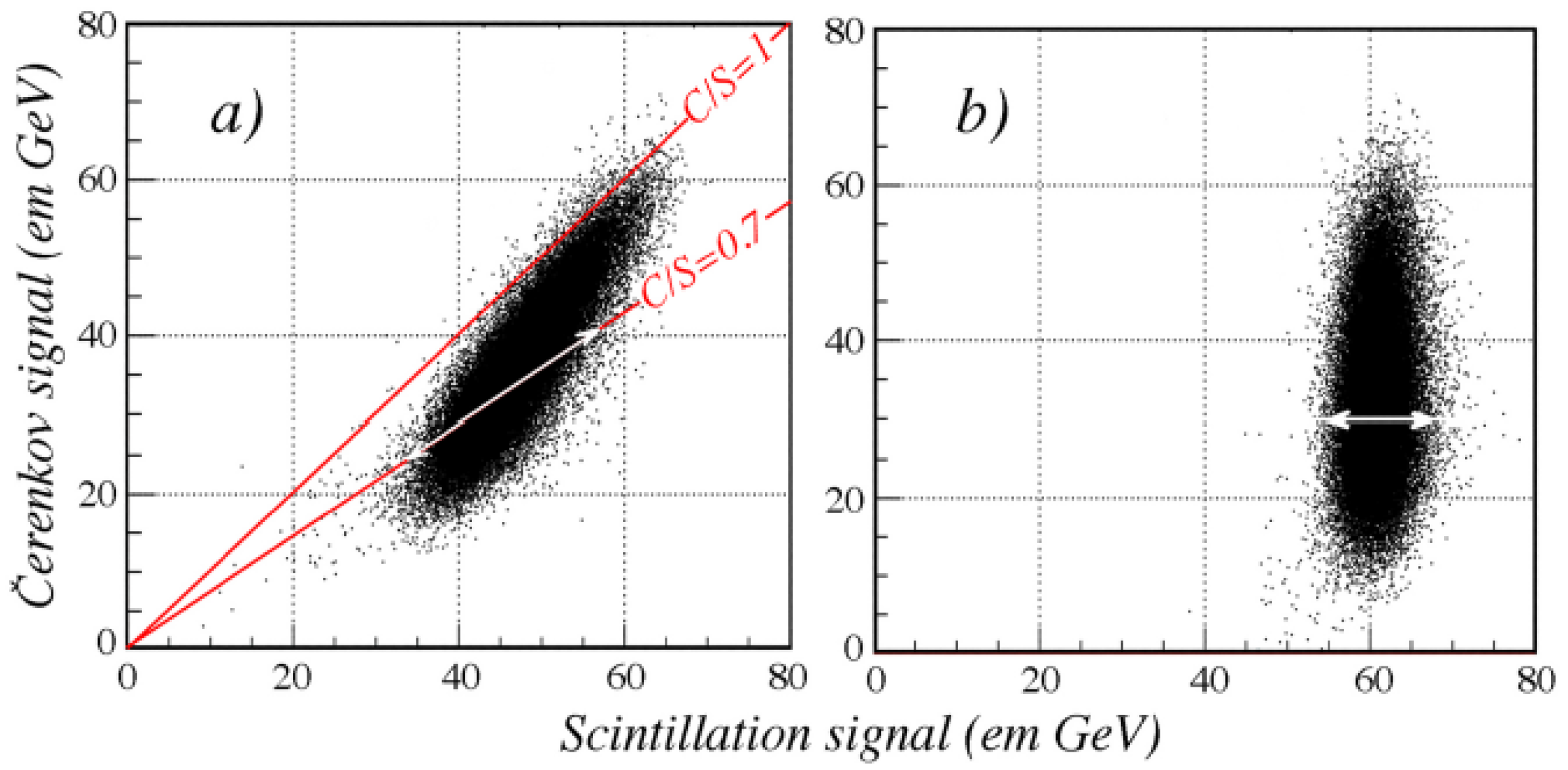
Figure 12 shows the signal distributions measured for 300 GeV pions (a) and protons (b), respectively. The signal distribution for protons is much more symmetric, as indicated by the Gaussian fit. This is because the em component of proton-induced showers is typically populated by
s that share the energy contained in this component more evenly than in pion-induced showers.The figure also shows that the rms width of the proton signal distribution is significantly smaller (by ∼20%) than for the pions.
Figure 12c shows that the average signal per GeV deposited energy is smaller for the protons than for the pions, by about 10%. This is also a consequence of the limitations on
production that affect the proton signals in this non-compensating calorimeter (
). So while the response to protons is smaller in this calorimeter, the energy resolution is better. Similar effects are expected to play a role for the detection of kaons, where
production is limited as a result of strangeness conservation in the shower development.
Whereas the phenomena discussed above are the result of differences in the electromagnetic shower component, which lead to differences in the response functions of the calorimeter to baryons, pions and kaons, other effects may also cause significant differences that at first sight might be unexpected. As an example, we mention the differences between electron and photon detection in a calorimeter. These are important, since the electromagnetic performance is typically experimentally studied with electron beams, whereas photon detection may be the most important goal
1. Showers initiated by high-energy photons and electrons are quite different in the early stage of the absorption process, before the shower maximum [
21].
The first effect results from the fact that the photons travel a certain distance (9/7 , on average) in the absorbing structure before they start losing energy, while electrons and positrons start losing energy immediately upon their entry. Moreover, the starting point of the photon-induced showers fluctuates from event to event, which leads to the second effect.
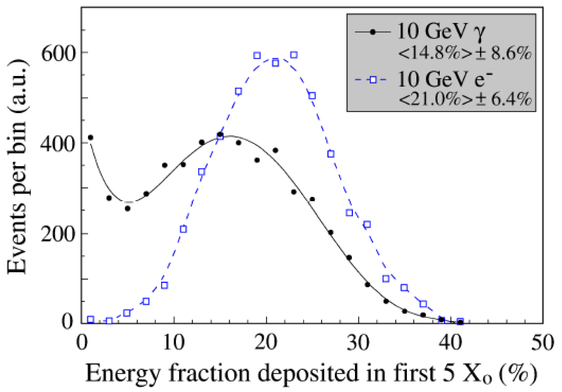
These effects are illustrated in
Figure 13, which shows the distribution of the energy deposited by 10 GeV electrons and 10 GeV photons in a
(2.8 cm) thick slab of lead. On average, the electrons deposit more energy in this material than the photons (2.10 GeV vs.1.48 GeV). However, the
fluctuations in the energy deposited by the photons are clearly larger than those in the energy deposited by the electrons (0.86 GeV vs.0.64 GeV). The distribution for the photon showers exhibits an excess near zero, which is the result of photons penetrating (almost) the entire slab without interacting. The “punch-thru” probability for a high-energy
is in this example
.
The different effects of dead material installed in front of the calorimeter on electrons/positrons and
s is relevant for experiments such as ATLAS, where the electromagnetic calorimeter is “hidden” in a cryostat, although the fact that this cryostat is made of aluminium makes the effects less dramatic than suggested in
Figure 13. Another consequence of the differences between electron and
induced showers is the fact that the very complicated calibration scheme that was developed for electrons showering in the three longitudinal segments of the ATLAS ECAL [
11] is
not necessarily the optimal solution for
detection in this calorimeter.
3.6. The Perceived Benefits of Longitudinal Segmentation
There is a deeply rooted belief that calorimeter systems for high-energy collider experiments should be longitudinally subdivided into several sections. As a minimum, one will usually want to have an electromagnetic and a hadronic section. A major reason for this belief is that such a subdivision is needed for recognizing em showers, and thus identify electrons and s entering the calorimeter.
This is a myth. It has been demonstrated repeatedly that there are several ways to identify em showers in longitudinally
unsegmented calorimeters. For example, the DREAM Collaboration has demonstrated four different methods that can be used to achieve this [
33]. These methods are based on
The measured lateral shower profile,
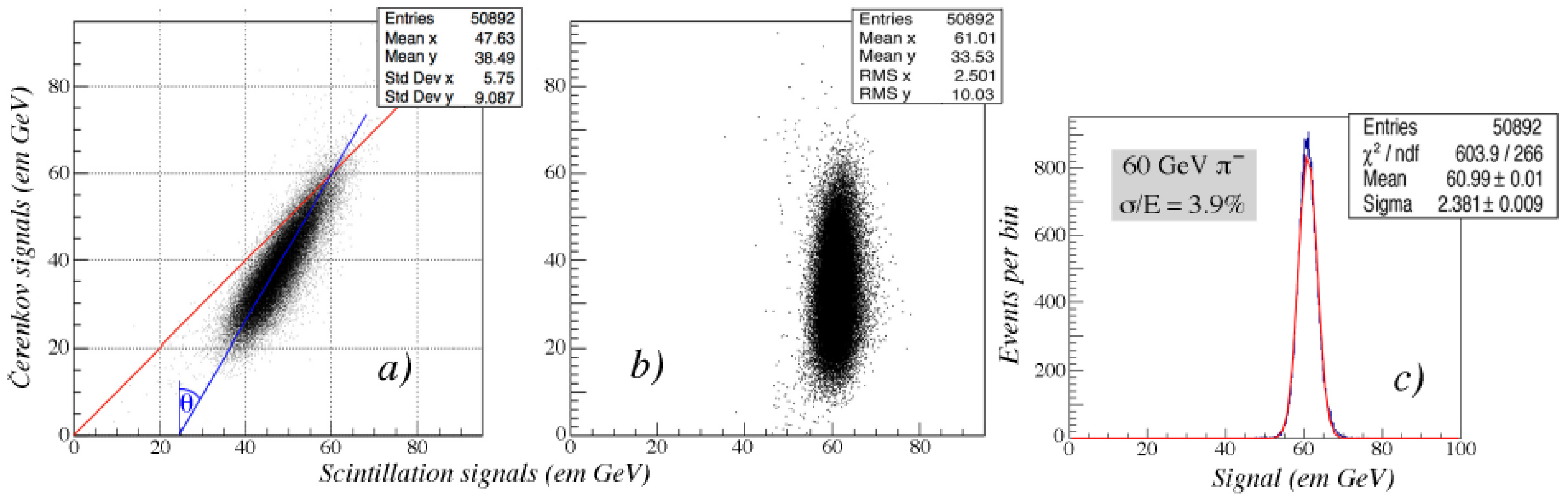
A comparison between the scintillation and Čerenkov signals produced by the developing shower,
The time structure of the signals, and in particular the starting time of the signals with respect to the signal produced in an upstream detector, or the pulse width.
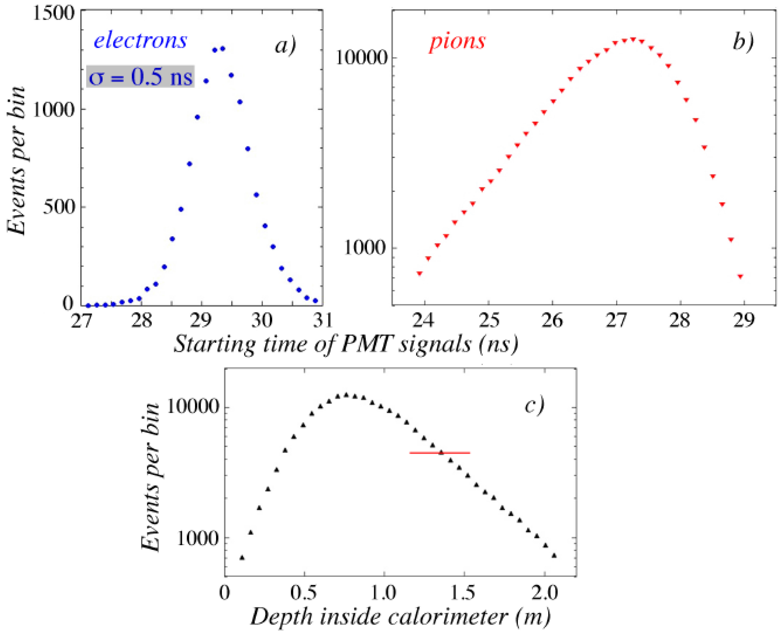
Figure 14 illustrates one of these methods, which is based on the starting time of the calorimeter signals, measured with respect to the signal produced by an upstream detector. This method is based on the fact that the light in the optical fibers travels at a lower speed than the particles that generate this light. The deeper inside the calorimeter the light is produced, the earlier the calorimeter signal starts. For the polystyrene fibers, the effect amounted to 2.55 ns/m. For the tested calorimeter, this led to a longitudinal position resolution of ∼20 cm.
Figure 14 shows the measured distribution of the starting time of the signals from 60 GeV
(
Figure 14a) and
(
Figure 14b). This pion distribution peaked ∼1.5 ns earlier than that of the electrons, which means that the light was, on average, produced 60 cm deeper inside the calorimeter. The distribution is also asymmetric, it has an exponential tail towards early starting times, i.e., light production deep inside the calorimeter. This signal distribution was also used to reconstruct the average depth at which the light was produced for individual pion showers. The result, depicted in
Figure 14c, essentially shows the longitudinal profile of the 60 GeV pion showers in this calorimeter.
It was shown in this paper that by combining all the available methods, which in several different ways exploited complementary information about the events, the longitudinally unsegmented RD52 fiber calorimeter could be used to identify electrons with a very high degree of accuracy. Using the time structure of the signals, the lateral shower profile and a comparison of the Čerenkov and scintillation signals, more than 99% of the electrons entering the detector were correctly identified with criteria that ruled out almost all hadronic particles as electron candidates. In practice, this is probably somewhat too optimistic, because of difficulties encountered in more realistic conditions than beam tests of prototype modules.
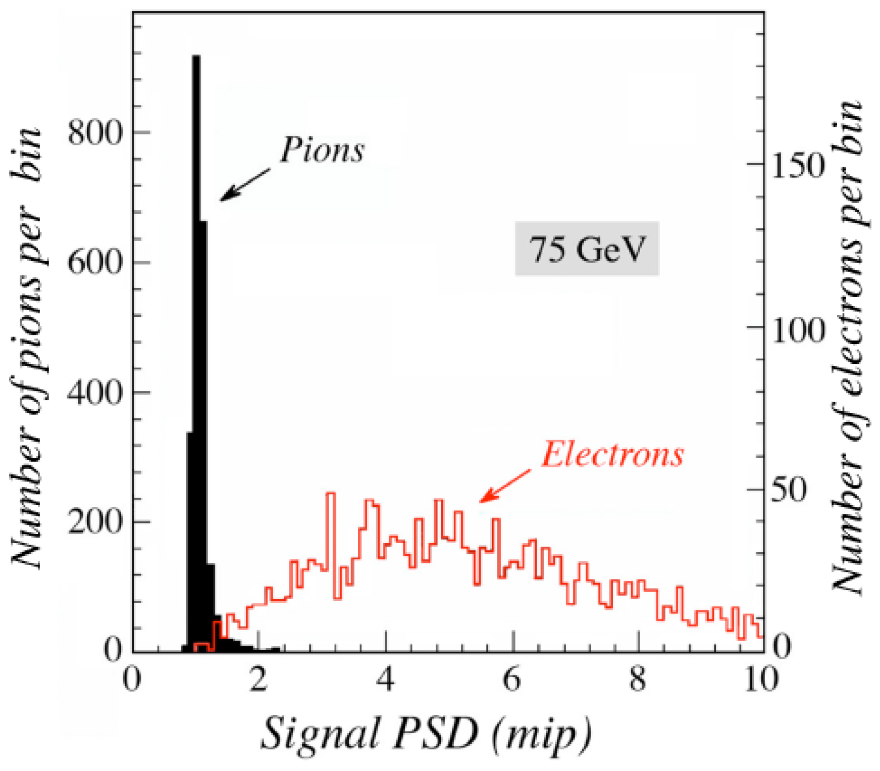
However, good electron/pion separation can already be achieved with much less sophisticated methods. Especially in beam tests, a very simple preshower detector (PSD), placed in front of the calorimeter, may do an adequate job. Such a device may consist of a plate of lead, 1 cm (1.9, 0.06) thick, followed by a sheet of plastic scintillator. When a beam consisting of a mixture of high-energy electrons and pions is sent through this device, almost all pions (96%) traverse it without strongly interacting. These pions produce a minimum ionizing peak in the scintillator. On the other hand, the electrons lose a considerable fraction of their energy by radiating large numbers of bremsstrahlung photons. Some of these photons convert into pairs in the PSD and thus contribute to the scintillation signals produced by this device.
The result is a very clear separation between electrons and pions.
Figure 15 shows the signal distributions for 75 GeV electrons and pions in the described device, used in beam tests of the CDF Plug Upgrade calorimeter [
34]. Even with such simple devices, pion rejection factors of the order of one hundred are readily achieved. Longitudinal segmentation of the calorimeter is thus most definitely
not an essential requirement for this purpose.
Other reasons often used for longitudinal segmentation include the possibility to optimize the energy resolution of the em section, while limiting at the same time the cost of the hadronic section. However, in future experiments at the next generation high-energy lepton-lepton colliders, excellent energy resolution is needed for all particles, not just electrons. Since sampling fluctuations are a major limiting factor both for electrons and hadrons in well designed dual-readout calorimeters, it stands to reason to use the same high sampling fraction and frequency throughout the calorimeter. This uniform structure is also a crucial factor for eliminating the intercalibration problems, illustrated in Sections 2.1.1 and 2.2.3, that plague all longitudinally segmented non-compensating calorimeter systems [
2,
13]. Traditionally, one has tried to tackle these problems by means of Monte Carlo simulations, but the results of such simulations leave very much to be desired [
35].
Elimination of longitudinal segmentation also offers the possibility to make a finer lateral segmentation with the same number of electronic readout channels. This has many potential benefits. A fine lateral segmentation is crucial for recognizing closely spaced particles as separate entities. Because of the extremely collimated nature of electromagnetic showers
2, it is also a crucial tool for recognizing electrons in the vicinity of other showering particles. Moreover, a fine lateral segmentation is important for the identification of electrons in general. Unlike the vast majority of other calorimeter structures used in practice, the RD52 fiber calorimeter offers almost limitless possibilities for lateral segmentation. If so desired, one could read out every individual fiber separately. Modern silicon PM technology certainly makes that a realistic possibility.


