Connecting Complex Electronic Pattern Formation to Critical Exponents

Abstract

Scanning probes reveal complex, inhomogeneous patterns on the surface of many condensed matter systems. In some cases, the patterns form self-similar, fractal geometric clusters. In this paper, we advance the theory of criticality as it pertains to those geometric clusters (defined as connected sets of nearest-neighbor aligned spins) in the context of Ising models. We show how data from surface probes can be used to distinguish whether electronic patterns observed at the surface of a material are confined to the surface, or whether the patterns originate in the bulk. Whereas thermodynamic critical exponents are derived from the behavior of Fortuin–Kasteleyn (FK) clusters, critical exponents can be similarly defined for geometric clusters. We find that these geometric critical exponents are not only distinct numerically from the thermodynamic and uncorrelated percolation exponents, but that they separately satisfy scaling relations at the critical fixed points discussed in the text. We furthermore find that the two-dimensional (2D) cross-sections of geometric clusters in the three-dimensional (3D) Ising model display critical scaling behavior at the bulk phase transition temperature. In particular, we show that when considered on a 2D slice of a 3D system, the pair connectivity function familiar from percolation theory displays more robust critical behavior than the spin-spin correlation function, and we calculate the corresponding critical exponent. We discuss the implications of these two distinct length scales in Ising models. We also calculate the pair connectivity exponent in the clean 2D case. These results extend the theory of geometric criticality in the clean Ising universality classes, and facilitate the broad application of geometric cluster analysis techniques to maximize the information that can be extracted from scanning image probe data in condensed matter systems.

1. Introduction

Since their invention in 1982, scanning probes have revolutionized our understanding of materials and their surfaces, yielding an ever increasing wealth of data available for in-depth analysis, on a wide variety of systems [1]. At least seventeen types of scanning probes have been developed [2,3], revealing new information about quantum materials via, e.g., scanning tunneling microscopy [4,5,6], scanning near-field optical microscopy [7,8], scanning X-ray methods [9,10,11], and atomic force microscopy [12], among others. Theory has been sprinting to catch up in order to interpret it all, and also to discover new ways of extracting information from the data, in order to fully realize this promise of new knowledge from the increasing variety of scanning probes and their ever-increasing experimental capabilities. While scanning probes have varying penetration depths, and therefore varying native ability to probe at least some of the bulk, their real strength lies in the exquisite spatial resolution at the surface. To date, the majority of theoretical treatments have focused on microscopic physics [2], with few theoretical treatments offering guidance for how to interpret the wealth of information [13] available in the multiscale pattern formation often observed on surfaces. We have recently pioneered a new set of techniques for analyzing scanning probe data by mapping two-component image data to random Ising models [14], based on geometric cluster methods imported from disordered statistical mechanics. A geometric cluster is defined as a set of aligned nearest-neighbor sites. The key insight is that near criticality, the spatial configurations of geometric clusters are controlled by the critical fixed point, and therefore the geometric properties encode critical exponents. The method is capable of extracting information from experimental data about disorder, interactions, and dimension. We have already successfully applied this new technique to uncover a unification of the fundamental physics governing the multiscale pattern formation observed in two disparate strongly correlated electronic materials (cuprate superconductors [14,15] and vanadium dioxide [16]).

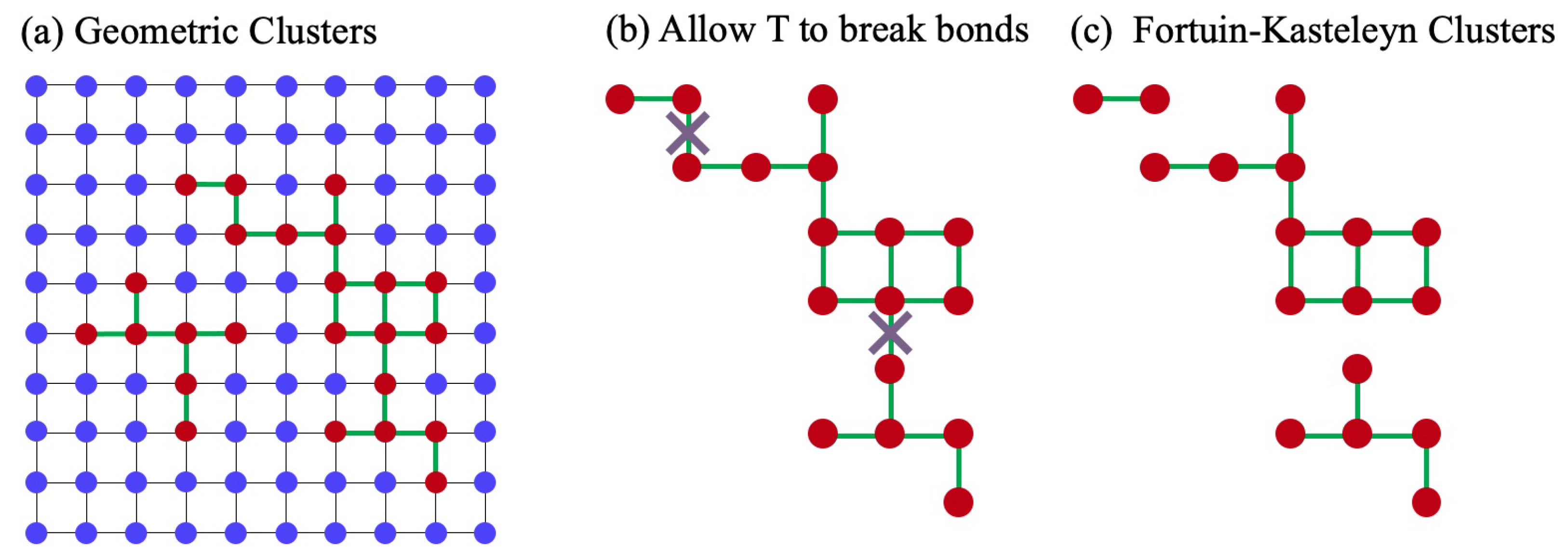
However, because it is the Fortuin–Kasteleyn (FK) clusters (See Figure 1) which encode thermodynamic criticality [17], rather than the geometric clusters which are directly accessible experimentally via scanning probes and which we employ in our method, little is known about the general theoretical structure of geometric clusters in clean and random Ising models, and the critical exponents associated with the geometric clusters are unknown for many of the fixed points which are key to interpreting experimental data. In this paper, we advance the theory of criticality as it pertains to geometric clusters in clean Ising models to further develop geometric cluster analysis techniques [14], in order to maximize the information that can be extracted from experiments using these new methods. Although the geometric clusters do not encode thermodynamic criticality, we conjecture that when the geometric clusters percolate, whether at or below the thermodynamic critical temperature, the geometric clusters do encode geometric criticality, complete with its own set of critical exponents, which we further conjecture are distinct from the exponents of uncorrelated percolation when arising in the context of an interacting model.

This paper is organized as follows. We first describe in Section 2 the model under consideration. We then ask in Section 3 whether the pair connectivity function can be a power law in any system other than uncorrelated percolation (to which we will answer “yes”). In Section 4, we present some conjectures considering geometric criticality as distinct from thermodynamic criticality. Next, we present in Section 5 our results for the critical geometric cluster exponents on 2D slices of the clean 3D Ising model (denoted by C-3Dx, where x means cross-section), and in Section 6 our simulations of the pair connectivity function of the clean 2D Ising model (denoted by C-2D). In Section 7 we discuss the relation of the order parameter in a 3D ferromagnetic Ising model to the percolation of geometric clusters on 2D slices of the 3D system and derive that the position of the 2D slice geometric cluster percolation point coincides with bulk critical point. In Section 8 we discuss the implications of the pair connectivity length scale in Ising models. Finally, in Section 9, we discuss and summarize our findings about geometric criticality, and present conclusions in Section 10. In addition, a List of Symbols can be found in

Table 1. List of symbols.

Symbol	Definition
${\sigma }_i$	Ising variable on a site i (Equation (1))
$J^{\left|\right|}$; $J^{\perp }$	In-plane and inter-plane Ising coupling constant (Equation (1))
h	Applied (uniform) magnetic field (Equation (1))
$h_i$	Random (local) field (Equation (1))
s	Number of sites in a nearest-neighbor connected cluster
h	Number of sites on the hull of a cluster
$R_s$	Radius of Gyration of a cluster (Equation (2))
$R_h$	Radius of Gyration of the interior of a cluster (Equation (3))
$D\left(s\right)$	Distribution of cluster sizes
$g_{\mathrm{conn}}\left(r\right)$	Pair connectivity function (Equation (4))
$g_{\mathrm{spin}}\left(r\right)$	Spin-spin correlation function (Equation (10))
${\xi }_c$	Spin-spin correlation length (Equation (11)
${\xi }_p$	Percolation correlation length (Equation (4))
2D	Two-dimensional
3D	Three-dimensional
C-2D	Clean 2D Ising model (i.e., no disorder)
C-3D	Clean 3D Ising model
C-3Dx	Interior slice of C-3D
T	Temperature
$T_c$	Magnetic ordering temperature
$T_p$	Percolaton temperature
$T_p^{\mathrm{slice}}$	Percolation temperature on a slice
$T_c^{3D}$; $T_p^{3D}$	Bulk (3D) $T_c$ and $T_p$
$T_c^{3D}(L\to \infty )=4.51152786J$	$T_c$ of C-3D in large system limit [19,20]
$T_c^{2D}(L\to \infty )=2/\ln (1+\sqrt{2})J$	$T_c$ of C-2D for infinite size system [21]
p	Percolation fraction
$p_c$	Critical fraction for percolation
FK	Fortuin–Kasteleyn
L	Length of one side of simulation
d	Spatial dimension
R	Infinite network strength (Equation (5))
$R_{\uparrow }^{slice}$; $R_{\downarrow }^{slice}$	Ininite network strength of up (down) spins on a slice (Equation (5))
${\pi }_i$; ${\tilde{\pi }}_i$	Lattice gas variables (Equation (6))
${\tilde{\gamma }}_i^{\infty }$	Characteristic function that spin i belongs to the infinite 2D slice $(+)$-cluster
${\gamma }_i^{\infty }$	Characteristic function that spin i belongs to the infinite 2D slice $(-)$-cluster

, and a List of Critical Exponents can be found in

Table 2. List of critical exponents, defined in terms of scaling relations near criticality.

Name	Symbol	Definition
Fisher Exponent	$\tau$	$D\left(s\right)\propto s^{\tau }$
Volume Fractal Dimension	$d_v$	$s\propto R_s^{d_v}$
Hull Fractal Dimension	$d_h$	$h\propto R_h^{d_h}$
	$\beta$	$M\sim |T-T_c{|}^{\beta }$
	$\nu$	$\xi \sim |T-T_c{|}^{-\nu }$
Anomalous Exponent for Magnetism (Equation (10) and (11))	${\eta }_c$	$g_{\mathrm{spin}}\left(r\right)\sim r^{-(d-2+{\eta }_c)}$
Anomalous Exponent for Percolation (Equation (4))	${\eta }_p$	$g_{\mathrm{conn}}\left(r\right)\sim r^{-(d-2+{\eta }_p)}$
${\eta }_c$ and ${\eta }_p$ as measured on a 2D (interior) slice	${\eta }_c^{\left|\right|}$; ${\eta }_p^{\left|\right|}$

.

2. The Model

In strongly correlated electronic systems, the combination of disorder and strong correlations can drive complex pattern formation [13], but disentangling correlations from disorder in the experimental system is an open problem. Recently, we have developed new cluster analysis techniques for interpreting scanning image probe data [14] in cases where the spatial data can be abstracted to two components (and thus may be mapped to an Ising variable [22,23]), and where the resulting cluster patterns display structure on multiple length scales.

Scanning probe experiments often reveal complex pattern formation at the surface of strongly correlated electronic systems [13,24]. For example, charge stripe orientations display complex geometric patterns at the surface of some cuprate superconductors, as revealed by scanning tunneling microscopy [5,25]. Complex patterns have also been observed in thin films of VO₂ and NdNiO₃ as they transition from metal to insulator, via scanning near-field optical microscopy [7,8,26] and via scanning X-ray microscopy [9]. Using the cluster analysis techniques we developed, we showed that in these cases the dominant type of disorder driving the pattern formation is in the random field [27] universality class, and we argued that this is the origin of nonequilibrium behavior in both systems [8,9,14,15,16].

In this paper, we expand the diagnostic toolset of the geometric cluster analyses we have developed to include the functional form and qualitative behavior of the connectivity function, derived directly from geometric clusters. We find that the pair connectivity function can be a power law at more than just uncorrelated percolation points, and we compute the corresponding critical exponent via Monte Carlo simulations.

We consider a short-range Ising model:

$$H=-J\sum _{\langle ij\rangle }{\sigma }_i{\sigma }_j,$$

(1)

where the sum runs over the sites of a cubic lattice for 3D systems, and over a square lattice for 2D systems, chosen with spacing at least as small as the resolution of the images to be studied. The tendency for neighboring regions in the data image to be of like character is modeled as a nearest neighbor ferromagnetic interaction J.

The Ising variable ${\sigma }_i=\pm 1$ on each coarse-grained site represents one of the two possible states, such as the two possible electron nematic orientations in the cuprates, or the two states of conductivity (metallic or insulating) in VO₂. For the two examples above, our cluster analysis [14,15,16] of the image data shows that the geometric clusters (which are defined as the connected set of the nearest neighbor sites with Ising variables being the same value) extracted from the multiscale pattern formation display universal scaling behavior over multiple decades, suggesting criticality and universality as the origin of the spatial complexity revealed by scanning probe microscopy in strongly correlated electronic systems. By comparing the data-extracted critical exponents derived from the self-similarity of the geometric clusters with the theoretical values for the fixed points contained in Equation (1), we have shown [14] that it is possible to identify the universality class governing the scaling behavior of the geometric clusters observed on surfaces of novel materials.

Once the universality class driving the pattern formation has been identified, this in turn yields information about the relative importance of disorder and interactions, the dominant type of disorder in the system, and the dimension of the phenomenon studied [14,15,16,25]. For example, by extracting the critical exponents associated with the geometric clusters appearing at the surface of a material, it is possible to understand whether those clusters are forming merely due to surface effects, or whether the clusters form throughout the bulk of the material and then intersect the surface, because the critical exponents are sensitive to dimension.

3. Where Is the Connectivity Function Power Law?

Although geometric clusters do not encode thermodynamic criticality, we claim that whenever the geometric clusters percolate, the resulting power law behavior encodes a type of geometric criticality [28,29]. We further claim that such geometric critical points in interacting models are new, distinct fixed points, which are different from uncorrelated percolation, as supported by our results to be presented in this paper. The pair connectivity function, derived from geometric clusters, is known to be power law at uncorrelated percolation points. The pair connectivity function $g_{\mathrm{conn}}\left(r\right)$ is defined as the probability that two sites separated by a distance r belong to the same connected finite cluster. Can it also be power law at certain fixed points in interacting models? The most natural clusters to define in Ising models are the geometric clusters, defined by nearest-neighbor sets of like Ising “spins”. The geometric clusters have the advantage that they are directly accessible in image probe data in a two-component system, and they are the clusters we employ in our method.

However, geometric clusters in Ising models are still poorly understood theoretically, presumably because they do not necessarily percolate at the thermodynamic transition temperature, $T_c$. Rather, it is the FK clusters which percolate at the thermodynamic transition temperature $T_c$, and which encode the thermodynamic critical behavior [17]. The FK clusters also constitute the critical “droplets” of the Fisher droplet model [30]. In the case of the clean 2D Ising model (C-2D), it has been shown that the geometric clusters also percolate at the thermodynamic transition, where the percolation temperature $T_p$ is equal to the thermodynamic transition temperature: $T_p=T_c$ [28]. In other cases, such as the clean and random bond Ising models in three dimensions, it has been shown that the bulk geometric clusters percolate at a temperature $T_p<T_c$, inside the ordered phase [28,29,31,32].

For the thermodynamic fixed points of Equation (1) at which $T_p=T_c$ (as happens at C-2D), the geometric clusters have well-defined fractal dimensions [33], both fractal volume dimension $d_v$ and fractal hull dimension $d_h$. In addition, geometric clusters defined on a 2D slice of the clean 3D Ising model also display fractal behavior [34]. At these points, because of their fractal structure, the large-scale geometric clusters are self-similar, i.e., they look the same on all length scales. This is a tell-tale characteristic of power law behavior, which leads us to our first conjecture:

Conjecture #1:

The connectivity function is a power law at all critical points for which the geometric clusters have fractal dimensions, $d_v$ and $d_h$.

Our results in Section 6 indicate that indeed the connectivity function is a power law at the C-2D critical fixed point, in support of Conjecture #1. This is of course implicit in the pioneering work of Coniglio and coworkers on the percolation of geometric clusters in this model [28,35]. Our results in Section 5 show that the connectivity function is also a power law on a 2D slice as the clean 3D Ising system passes through thermodynamic criticality at $T_c^{3D}$. (See Figures 5 and 6). It was already known from the work in Ref. [34] that geometric clusters defined on a 2D slice have well-defined fractal dimensions at $T_c^{3D}$ in the clean 3D Ising model, lending further support to Conjecture #1.

4. Geometric Criticality and Thermodynamic Criticality: Two Types of Critical Exponents

It is known that at the clean 2D Ising (C-2D) fixed point, there are two distinct sets of critical exponents: one set associated with the thermodynamic criticality and encoded by the FK clusters, and a different set associated with “geometric criticality”, encoded by the geometric clusters [17,28,33]. As both types of clusters percolate right at the transition temperature, $T_p=T_c$, both types of clusters exhibit power law behavior, yielding two distinct sets of critical exponents, one set derived from each type of cluster. While the scaling laws governing the exponent relations at this fixed point are the same for the two types of clusters, the values of the geometric exponents are not equal to the values of the thermodynamic exponents, and neither set is equal to the values of uncorrelated percolation exponents. In this sense, the C-2D fixed point is therefore both a thermodynamic critical point and a type of geometric critical point. This also implies that there are two order parameters for the 2D clean Ising model (the magnetization and the infinite geometric cluster); as we will show below, corresponding to the two order parameters are two distinct length scales.

The set of critical exponents derived from the thermodynamic order parameter (in this case, the magnetization), is associated with percolation of the FK clusters, and encodes thermodynamic criticality—we will denote these exponents by the subscript “c” (to match the “c” in the thermodynamic critical temperature $T_c$). This type of exponent has been widely discussed in the literature. The other set of exponents is derived from the percolation order parameter, which is the infinite network strength, defined as the ratio of the number of sites in the infinite connected geometric cluster to the total number of sites in the system. This second set of critical exponents is associated with percolation of geometric clusters, and encodes geometric criticality—we will denote these exponents by the subscript “p” (for percolation).

The fact that there can be two distinct sets of exponents has been largely ignored in the literature, except at the C-2D [28,33] fixed point where $T_p=T_c$, and in the clean 3D Ising model [31,36] where $T_p<T_c$. The percolation temperature is also known to be inside the ordered phase $T_p<T_c$ in 3D random bond Ising models, as well [28,29,31,32]. When $T_p<T_c$, we claim that as the geometric clusters percolate at $T_p$, they display a type of criticality, even though the system is not at the thermodynamic critical point. To understand why, it is first helpful to have an intuition about how $T_p$ in an interacting model is related to uncorrelated percolation. The relation of the percolation temperature $T_p$ to $T_c$ is constrained by the site percolation thresholds in the uncorrelated case: on a square lattice, the percolation threshold is $p_c=0.59$, while on a cubic lattice, it is $p_c=0.31,$ where p is the fraction of sites that are occupied. (In the Ising case, p becomes the fraction of sites with aligned spins [28].)

The high temperature limit of Equation (1) maps to uncorrelated percolation with $p=0.5$. So, in 2D, neither up nor down spins percolate at $T\to \infty ,$ since $p(T\to \infty )=0.5<p_c=0.59$ on a square lattice. Since a majority geometric cluster spans the system in the ordered phase, it must pass through a percolation point at $T_p=T_c$ if the transition is continuous. Indeed, it has been proven rigorously that $T_p=T_c$ in clean 2D Ising models [28]. Consistent with the argument above, it is known that ${\Delta }_p={\Delta }_c=0$ in the 2D random field Ising model [37] where $\Delta$ is the disorder strength. We expect similar physics to obtain in the random bond Ising model in two dimensions.

In three dimensions, the high temperature limit of Equation (1) still maps to uncorrelated site percolation with $p=0.5$, but now both up and down spins span the system, since $p(T\to \infty )=0.5>p_c=0.31$ on a cubic lattice, where $p_c$ is the site percolation threshold. Upon decreasing temperature, the majority clusters grow below $T_c$, but since they were already spanning the system, the majority clusters do not pass through a percolation point. However, the minority geometric clusters must pass through a percolation point as they begin to shrink below $T_c$, although there is no obvious reason why they should do so at $T_c$. In fact, in the clean 3D case, it has been rigorously shown that $T_p<T_c$ [31]. This inequality also holds in the random bond case as well [32].

At C-2D, the two sets of critical exponents separately satisfy the same scaling relations. For example, as discussed in Refs. [28,33], the familiar exponent relations $d-2+\eta =2\beta /\nu =2(d-d_v)$ are satisfied by the thermodynamic exponents as $d-2+{\eta }_c=2{\beta }_c/{\nu }_c=2(d-d_{v,c})$, and the same exponent relations are separately satisfied by the connectivity function and the geometric clusters as $d-2+{\eta }_p=2{\beta }_p/{\nu }_p=2(d-d_{v,p})$. The thermodynamic exponents in this case are [38,39] ${\eta }_c=0.25$, ${\beta }_c/{\nu }_c=1/8$, and $d_{v,c}=15/8$, where the volume fractal dimension $d_{v,c}$ is derived from the fractal structure of the FK clusters at the critical point [33]. Inserting these values into the above scaling relations yields $2-2+0.25=2*(1/8)=2*(2-15/8)$, and the exponents are clearly self-consistent. The exponents associated with percolation of the geometric clusters are ${\beta }_p/{\nu }_p=5/96$ and $d_{v,p}=187/96$ [33], where the volume fractal dimension $d_{v,p}$ is derived from the fractal structure of the geometric clusters as they percolate at $T_p=T_c$. Inserting these values into the exponent relation $2{\beta }_p/{\nu }_p=2(d-d_{v,p})$ yields $2*(5/96)=2*(2-187/96)$, indicating that the geometric clusters also satisfy scaling relations at C-2D.

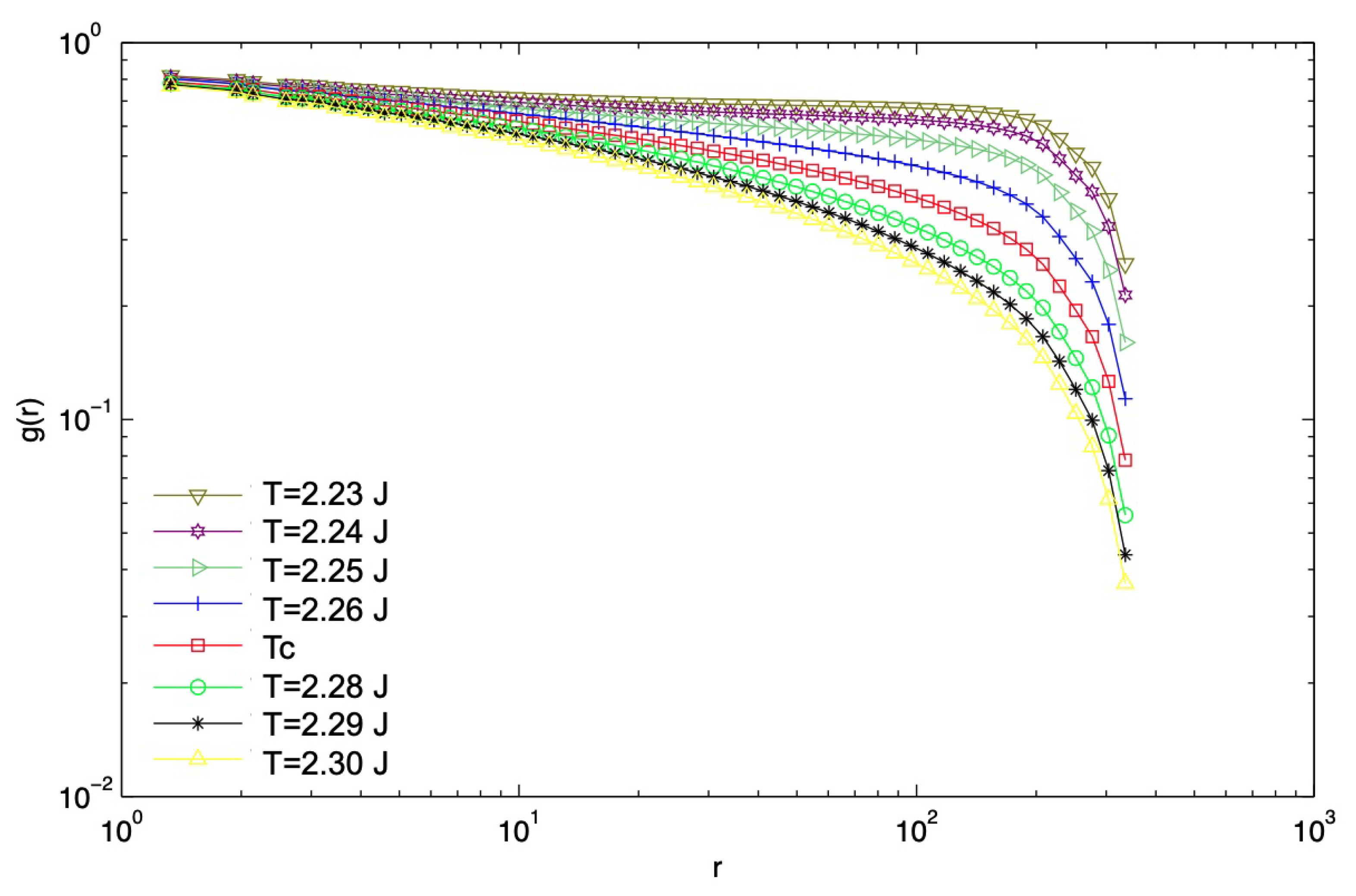
Although we have not found an explicit, direct calculation in the literature of the exponent ${\eta }_p$ at C-2D, which in this case should be derived from the pair connectivity function familiar from percolation theory, our results based on numerical simulations of the connectivity function $g_{\mathrm{conn}}\left(r\right)$ at C-2D indicate that $d-2+{\eta }_p=0.104\pm 0.002$ as shown in Figure 7, consistent within error bars with the scaling relation $d-2+{\eta }_p=2{\beta }_p/{\nu }_p$ ($0.104\pm 0.002\approx 2*(5/96)$). Thus, we see that at C-2D, there are two distinct sets of exponents, and that the geometric exponents also satisfy the scaling relations of criticality. This brings us to our second conjecture:

Conjecture #2:

There are two distinct sets of critical exponents which both satisfy scaling relations at all critical points for which $T_p=T_c$: one derived from the FK clusters, and the other derived from the geometric clusters.

5. Numerical Results for the Critical Exponents Defined on 2D Slices of a 3D System

We are ultimately interested in understanding the origin of the complex, two-component pattern formation observed at the surfaces of some strongly correlated electronic systems [13,14,16] via scanning image probes. In cases where the data show multiscale clusters of two distinct types, one of the drivers of such behavior can be proximity to a critical point of an Ising model, Equation (1). We focus in this paper on the clean Ising case; future work will include the effects of disorder. The problem at hand, then, is to map the properties of the observed geometric clusters to critical exponents of the model. We focus here on five exponents that can be directly extracted from the microscopy imaging data, and can be used to compare with different models to identify the universality class (explained more fully below): The Fisher exponent $\tau$ which describes the cluster size distribution; the volume fractal dimension $d_v$ and the hull fractal dimension $d_h$ of geometric clusters; the anomalous dimension ${\eta }_c^{\left|\right|}$ which controls the spin-spin correlation function; and as we will see below, ${\eta }_p^{\left|\right|}$ which controls the pair connectivity function.

We are interested in this section in the critical behavior displayed by the 2D slice geometric clusters near the 3D clean Ising phase transition (C-3Dx) which occurs at the bulk 3D transition temperature $T_c^{3D}$. (In Section 7 we will demonstrate that this temperature indeed coincides with the 2D slice percolation point $T_p^{slice}$.) The simulations of the clean Ising system are performed near $T_c^{3D}$ for the study of geometric criticality on 2D slices, and the Wolff single cluster algorithm [40] is known to be successful in mitigating critical slowing down effects near criticality. Therefore, we use this well-established cluster updating algorithm in our simulations. We adopt open boundary condition, because this representation is consistent with our context of microscopy experiments on real materials with finite scale. Throughout the paper, we use the logarithmic binning method which is a standard technique for analyzing the scaling behavior [41]. For the 3D cubic lattice, we use $T_c^{3D}=4.51152786J$ [19,20], and all simulations are performed using system sizes from $L^3={80}^3$ to $L^3={192}^3$ averaged over a large number of configurations in the Monte Carlo simulation in the order of magnitude ${10}^4$. We take samples of configurations every 1000 Wolff steps after the system reaches equilibrium, in order to mitigate explicit spatial correlations between different images. As one whole cluster is updated for each Wolff iteration, 1000 steps are empirically a large enough interval to make two neighboring sample images look totally different.

In the simulations, we have found that the percolation critical exponents extracted from $(+)$-clusters and $(-)$-clusters, respectively, are consistent with each other. This is expected, since at $T_p^{\mathrm{slice}}=T_c^{3D}$ there is $(+)/(-)$ symmetry (see Section 7). Therefore, we present the results with both clusters considered together for better statistics.

The cluster size distribution $D\left(s\right)$ measures the number of geometric clusters with a given size s, and scales with $s^{-\tau }$ as geometric clusters become critical. It is important to remember that when considered in the bulk context, geometric clusters do not display criticality at the bulk transition temperature $T_c^{3D}$, but rather the minority clusters experience a percolation transition (and therefore display criticality) (At high temperatures in three dimensions, both $(+)$ and $(-)$ clusters span the system, since the uncorrelated percolation transition in a cubic lattice occurs at a fraction of 31%. At very low temperatures in 3D, the system is spanned only by a majority cluster. The percolation transition for geometric clusters happens inside the ordered phase, $T_p^{3D}<T_c^{3D}$, when minority clusters cease to span the system) at a lower temperature $T_p^{3D}<T_c^{3D}$. However, we find that when a 2D slice of the system is considered, the geometric clusters as defined on the slice do display critical behavior in the form of power law scaling at the bulk transition temperature $T_c^{3D}$. For a 2D slice embedded in the 3D bulk system, we find that $D\left(s\right)\sim s^{-\tau }$ at $T_c^{3D}$, with the Fisher exponent $\tau$ specific for geometric clusters defined on a 2D cross section of a 3D system. With a finite field of view (FOV), $D\left(s\right)$ in the bulk is known to have a scaling bump, which skews $\tau$ to a lower value [42]. In order to mitigate this effect, we analyze $D\left(s\right)$ using only internal clusters, i.e., those which do not touch a boundary. $D\left(s\right)$ of the internal clusters shows unskewed power law behavior within a cutoff [43].

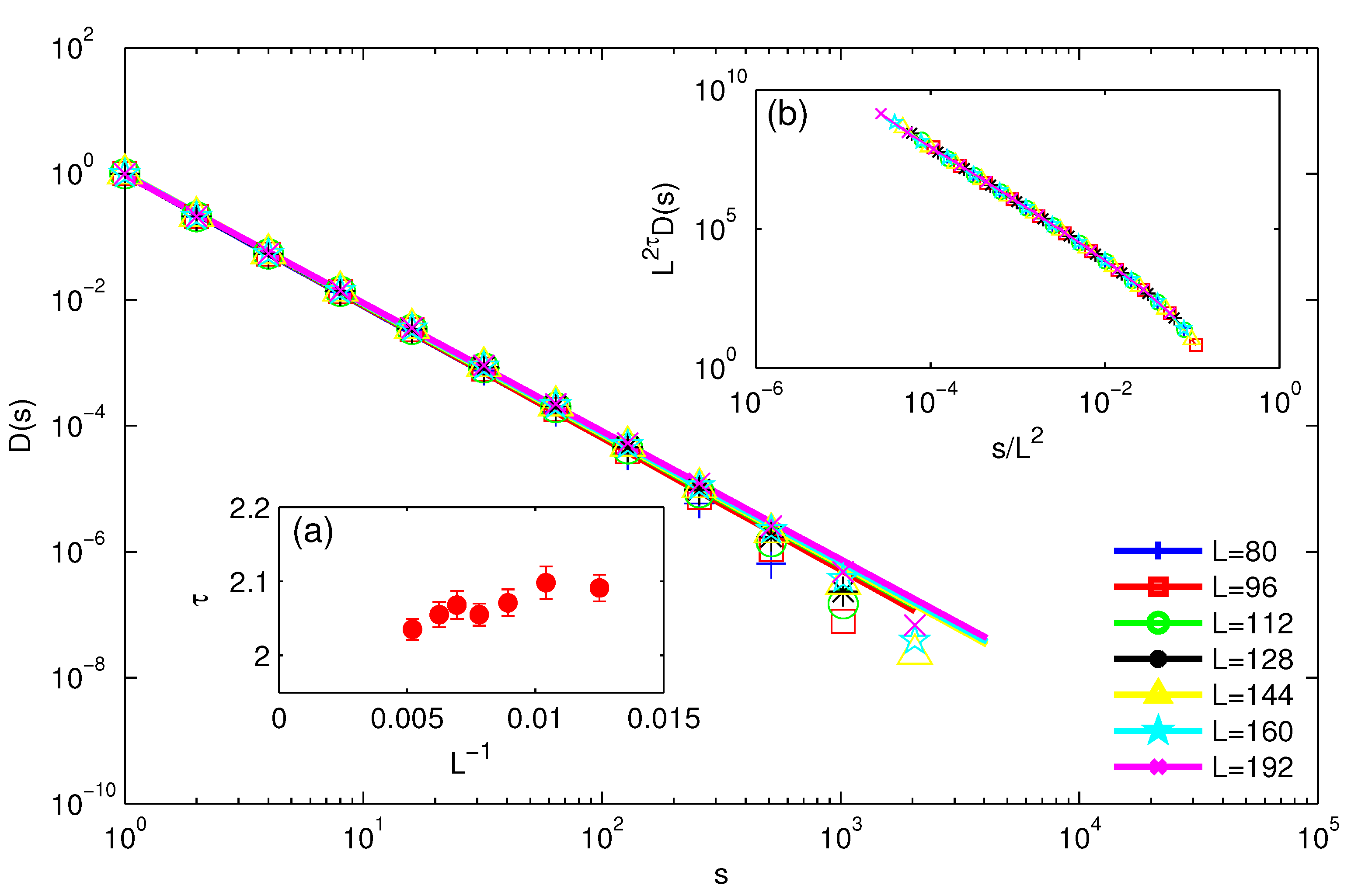
Figure 2 shows the cluster size distribution $D\left(s\right)$ of internal 2D cross-sectional clusters for different system sizes at $T_p^{\mathrm{slice}}=T_c^{3D}$. For each system size, we exclude the last two points, which deviate from power law scaling, and fit all the other points within this cutoff [43]. Based on the observed power law behaviors in Figure 2, we use the discrete logarithmic derivative method (DLD) [44] to extract $\tau$. Since we are only interested in the slope $-\tau$, we normalize all the $D\left(s\right)$ with $D(s=1)=1$ for better comparison between different system sizes. As can be seen in the figure, depending on the system size, power law scaling persists for about 2.5 decades of scaling. We extrapolate $\tau$ extracted at $T_c^{3D}$ to $L\to \infty$, and we find that a linear fit of ${\tau }^{\left(L\right)}$ yields $\tau =2.001\pm 0.013$ as $L\to \infty$. Here, the extrapolation follows the linear regression method with error-in-variables [45]. In general, the critical exponents cannot be directly obtained from a rigorous parametric fitting because the exact analytical form of the finite scaling functions are usually unknown. Under this case, linear extrapolation is a standard first-order approximation method for exponent extractions [46], and we use this for critical exponent extrapolations throughout the whole paper. The natural finite-size scaling hypothesis for the cluster size distribution at criticality reads $D(s,L)={\left(L^2\right)}^{-\tau }\widehat{\mathcal{D}}(s/L^2)$, where $\widehat{\mathcal{D}}$ is a universal scaling function [46]. The inset (b) in Figure 2 shows that using the exponent $\tau$ derived as above, the results from the main panel exhibit scaling collapse to a universal scaling function $\widehat{\mathcal{D}}$ as expected.

The cluster volumes s and hulls h become fractal near a percolation point. The fractal nature of the 2D cross-sectional cluster volumes at $T_p^{\mathrm{slice}}=T_c^{3D}$ can be described by $s\sim R_s^{d_v}$ with fractional rather than integer $d_v$ for $s\gg 1$. Here, $d_v$ is the volume fractal dimension, and $R_s$ is the radius of gyration of the cluster,

$$R_s^2\equiv \frac{1}{2}\sum _{i,j}{|{\mathbf{r}}_i-{\mathbf{r}}_j|}^2/s^2$$

(2)

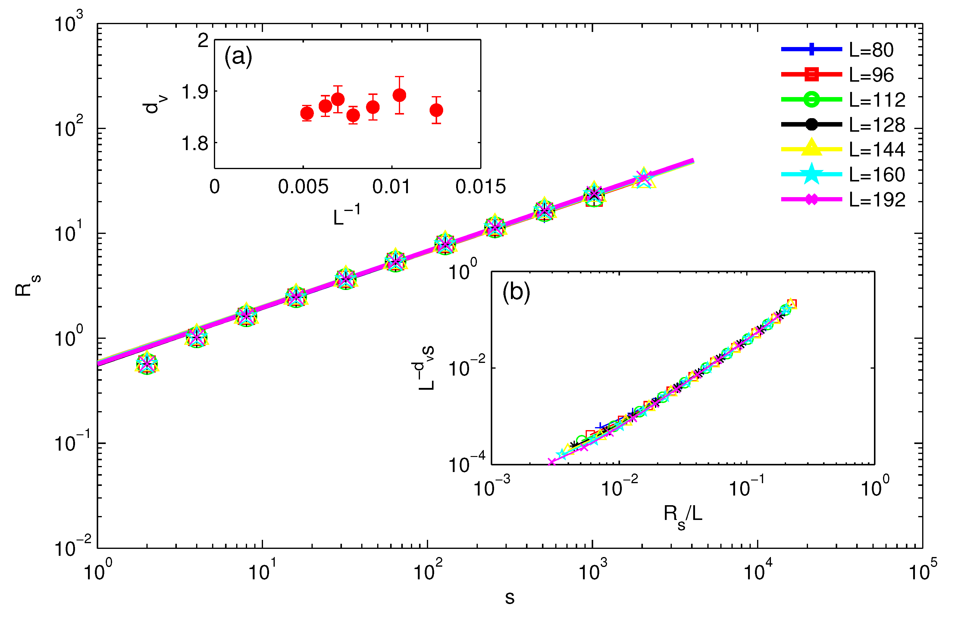
where the sum is over sites in the cluster, and ${\mathbf{r}}_i$ and ${\mathbf{r}}_j$ are the positions of the ith and jth sites [47]. Figure 3 shows a DLD power law fit of $s\sim R_s^{d_v}$, using only the internal clusters to mitigate boundary effects. Since the scaling relation is for $s\gg 1$, we exclude the first 3 points which correspond to the non-universal short-length regime. All the other points belong to the power law scaling regime. The power law fits at $T_p^{\mathrm{slice}}=T_c^{3D}$ persist for about two decades of scaling, depending on the system size. A straightforward fit extrapolating $d_v$ to the thermodynamic limit yields $d_v=1.856\pm 0.018$. The inset Figure 3b illustrates the scaling collapse for different system sizes to the universal function $\widehat{s}$ using the extrapolated values of $d_v$, based on the finite-size scaling hypothesis $s=L^{d_v}\widehat{s}(R_s/L)$ [46].

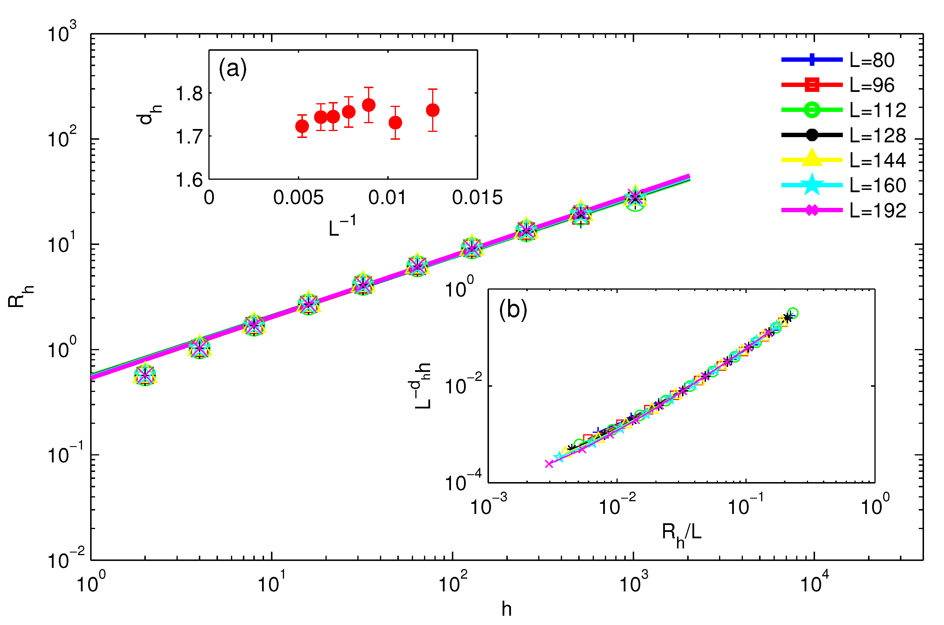
The cluster hulls h scale with $h\sim R_h^{d_h}$ near a percolation point. The clusters are said to be fractal if $d_h$ is fractional rather than integer. In this case, we are only tracking the outer (externally accessible) surfaces of each cluster. Thus, one surface might contain not only the cluster itself, but also the subclusters inside. Therefore, $R_h$ here refers to the radius of gyration of all the sites enclosed by the hull, including any subclusters:

$$R_h^2\equiv \frac{1}{2}\sum _{i,j\in \mathrm{h}}{|{\mathbf{r}}_i-{\mathbf{r}}_j|}^2/s^2$$

(3)

To mitigate the boundary effect, we still use only the internal clusters in the DLD fit. We exclude the first 2 point from the fit (h is a smaller measure than s for a cluster), which deviate from the power law scaling regime and correspond to non-universal short distance physics. As shown in Figure 4, the power law behavior extends over about 2 decades, depending on the system size. A straightforward fit extrapolating to the thermodynamic limit at $T_p^{\mathrm{slice}}=T_c^{3D}$ yields $d_h=1.714\pm 0.022$. The inset Figure 4b shows the scaling collapse for different system sizes to the universal function $\widehat{h}$ using the extrapolated values of $d_h$, based on the finite-size scaling hypothesis $h=L^{d_h}\widehat{h}(R_h/L)$ [46].

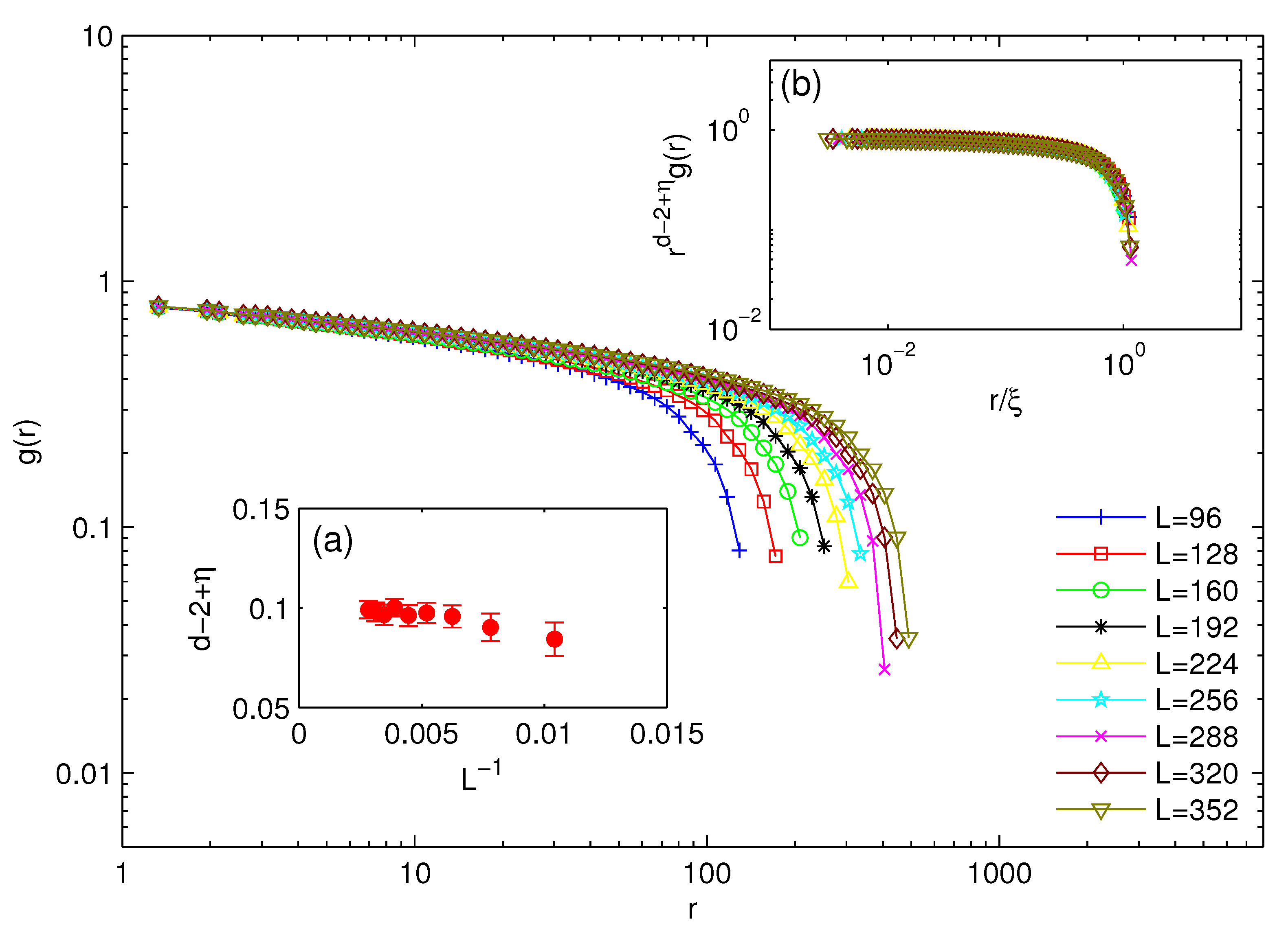
As introduced in the previous section, the pair connectivity function $g_{\mathrm{conn}}\left(r\right)$ is defined as the probability that two sites separated by a distance r belong to the same finite cluster. This correlation function scales with $g_{\mathrm{conn}}\left(r\right)\sim r^{-(d-2+{\eta }_p)}$ close to the percolation point. Figure 5 shows $g_{\mathrm{conn}}\left(r\right)$ at $T_p^{\mathrm{slice}}=T_c^{3D}$ with different system sizes. As shown by the figure, in addition to the power law behavior, associated with $g_{\mathrm{conn}}\left(r\right)$ there appears to be an exponential decay characterized by the correlation length scale of the finite system. Therefore, we infer the scaling form

$$g_{\mathrm{conn}}\left(r\right)\sim r^{-(d-2+{\eta }_p)}{e}^{-r/{\xi }_p}$$

(4)

with a finite correlation length, and then fit the curves in the main panel using this scaling form. From the fits, we find that the curves of $g_{\mathrm{conn}}\left(r\right)$ are consistent with the shape of the scaling form with some large percolation correlation length ${\xi }_p$ comparable with the finite system size. The inset (a) of Figure 5 shows the extracted anomalous dimension $d-2+{\eta }_p$ from the scaling form fits in the main panel. A straightforward fit extrapolating to $L\to \infty$ yields $d-2+{\eta }_p=0.322\pm 0.002$. The curves in the main panel collapse onto each other for the extrapolated $d-2+{\eta }_p$, as shown by the inset (b) of Figure 5.

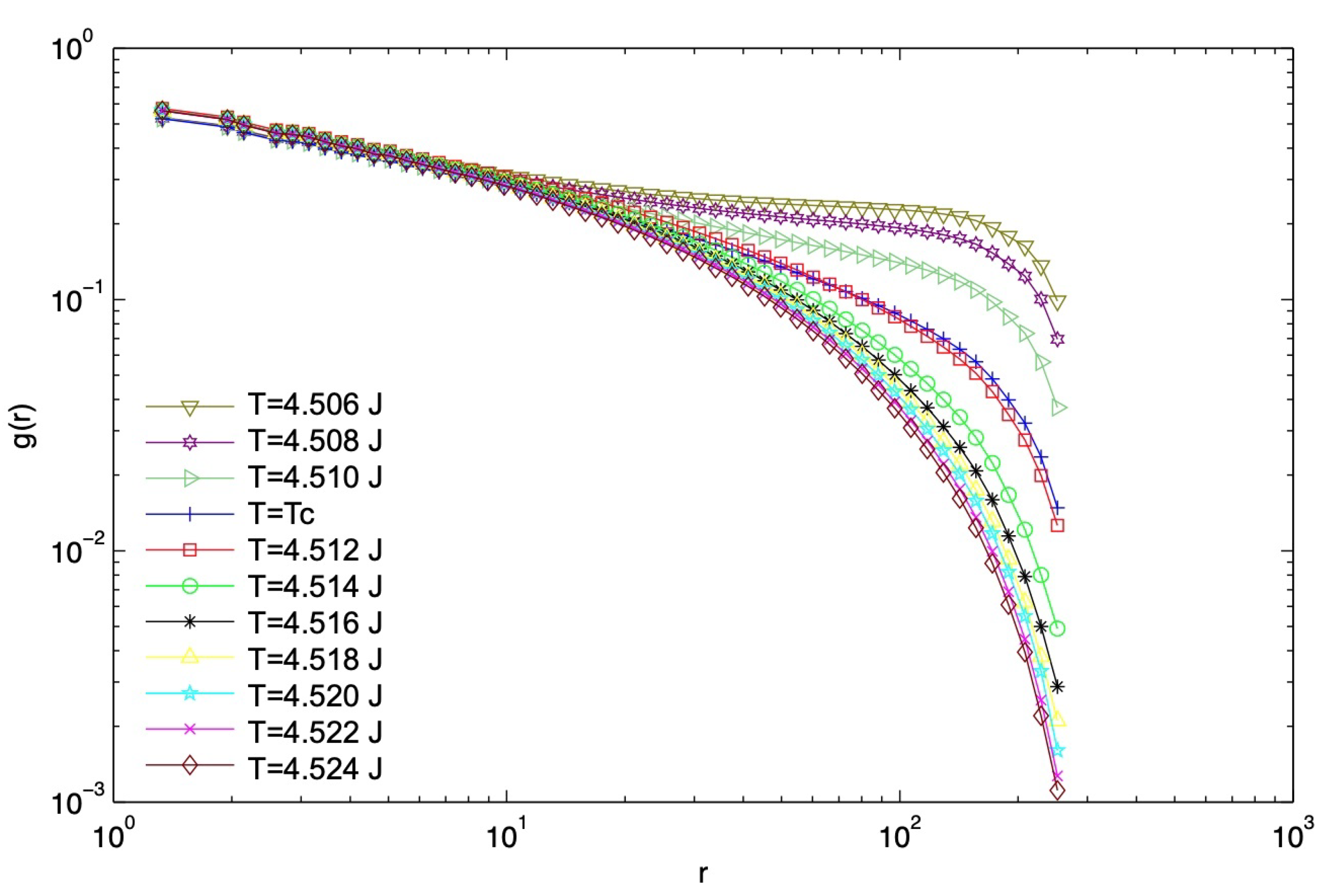
In Figure 6, we show the C-3Dx pair connectivity function $g_{\mathrm{conn}}\left(r\right)$ simulated with system size $L=192$ for different temperatures near $T_c^{3D}$. It is evident that for $T\gtrsim T_c^{3D}$, $g_{\mathrm{conn}}\left(r\right)$ is consistent with the shape of the scaling form in Equation (4) and for $T<T_c^{3D}$, $g_{\mathrm{conn}}\left(r\right)$ turns up at large r. For $g_{\mathrm{conn}}\left(r\right)$ calculated using all the possible pairs in the system, this up-turn is a characteristic behavior of the connectivity function when the system transitions from the “disordered side” (zero infinite network strength $R=0$) to the “ordered side” (non-zero infinite network strength $R>0$) through a percolation point, indicating the presence of an infinite cluster on a 2D slice. (Here R is the percolation order parameter defined on the 2D slice, also called the infinite network strength, and defined as the ratio of the number of sites in the infinite connected geometric cluster to the total number of sites in the system.) Therefore, this behavior can be used as a diagnostic tool to estimate the percolation point in an experimental situation. In the present case, this up-turn happens in the vicinity of $T_c^{3D}$, corroborating the idea that $T_p^{\mathrm{slice}}$ coincides with the bulk thermodynamic transition temperature, $T_p^{\mathrm{slice}}=T_c^{3D}$.

We have studied the scaling behavior of cross-sectional 2D slice geometric clusters embedded in the 3D bulk clean Ising system. We have found robust power law scaling (about two decades) for the measures related to the self-similarity of geometric clusters at $T_c^{3D}$, as well as the existence of universal scaling functions. All of these phenomena corroborate the conjecture that geometric criticality on a 2D slice occurs at the bulk critical temperature $T_p^{\mathrm{slice}}=T_c^{3D}$, and we have extracted the corresponding critical cluster exponents, as summarized in

Table 3. Theoretical/numerical values for the 2D geometric cluster self-similarity-characterized critical percolation exponents for Ising models and standard percolation model.

Model	2D Ising Model [33,48]	2D Slice of 3D Ising Model (This Work)	Standard Percolation [47,49,50]
Fixed Point	C-2D	C-3Dx	P-2D
$\tau$	$379/187=2.027$	$2.001\pm 0.013$	$187/91=2.055$
$d_v$	$187/96=1.948$	$1.856\pm 0.018$	$91/48=1.896$
$d_h$	$11/8=1.375$	$1.714\pm 0.022$	$7/4=1.75$
$d-2+{\eta }_p$	$0.104\pm 0.002$ (this work)	$0.322\pm 0.002$	$5/24=0.208$

.

6. Numerical Results for the Connectivity Function in the Clean 2D Ising Model

In the clean 2D Ising model, the percolation point coincides with the critical point, and both up and down geometric clusters percolate symmetrically at $T_p^{2D}=T_c^{2D}$ under zero external field [28,51]. The values of the exponents $\tau$, $d_v$ and $d_h$ are already given in the work by Janke et al. [33], as summarized in Table 3. In the present work, we simulate the connectivity function in order to obtain the value of the anomalous dimension $d-2+{\eta }_p$. Figure 7 shows the connectivity function $g_{\mathrm{conn}}\left(r\right)$ at $T_p^{2D}=T_c^{2D}$, with $T_c^{2D}=1/ln(1+\sqrt{2})$ for the square lattice [52]. The inset (a) shows $d-2+{\eta }_p$ extracted from the scaling form fit of the connectivity function $g_{\mathrm{conn}}\left(r\right)\sim r^{-(d-2+{\eta }_p)}{e}^{-r/{\xi }_p}$ at $T_c^{2D}$ for different system sizes, and a straightforward fit extrapolating to the thermodynamic limit gives $d-2+{\eta }_p=0.104\pm 0.002$. With this value, all of the curves in the main panel collapse on top of each other, as shown by the inset (b). Figure 8 shows the behavior of $g_{\mathrm{conn}}\left(r\right)$ around $T_c^{2D}$ with system size fixed at $L=256$. As for the case of C-3Dx, we find that for $T>T_c^{2D}$, the pair connectivity function $g_{\mathrm{conn}}\left(r\right)$ is consistent with the scaling form shape and for $T<T_c^{2D}$$g_{\mathrm{conn}}\left(r\right)$ turns up. This change of behavior happens in the close vicinity of $T_c^{2D}$, consistent with the idea that $T_p^{2D}=T_c^{2D}$.

7. Relation of Infinite Cluster to Bulk Magnetization on a 2D Slice

The bulk minority geometric clusters for the clean 3D Ising model are known to percolate inside the ordered phase, with the percolation temperature $T_p^{3D}=0.93T_c^{3D}<T_c^{3D}$ [31,36]. Therefore, the bulk geometric clusters do not display fractal properties at the critical temperature $T_c$, although they do at $T_p^{3D}$. At first glance, one might think that the geometric clusters on a 2D slice, which are cross-sections of the 3D bulk clusters, should also display critical scaling behavior at the bulk percolation temperature $T_p^{3D}$. 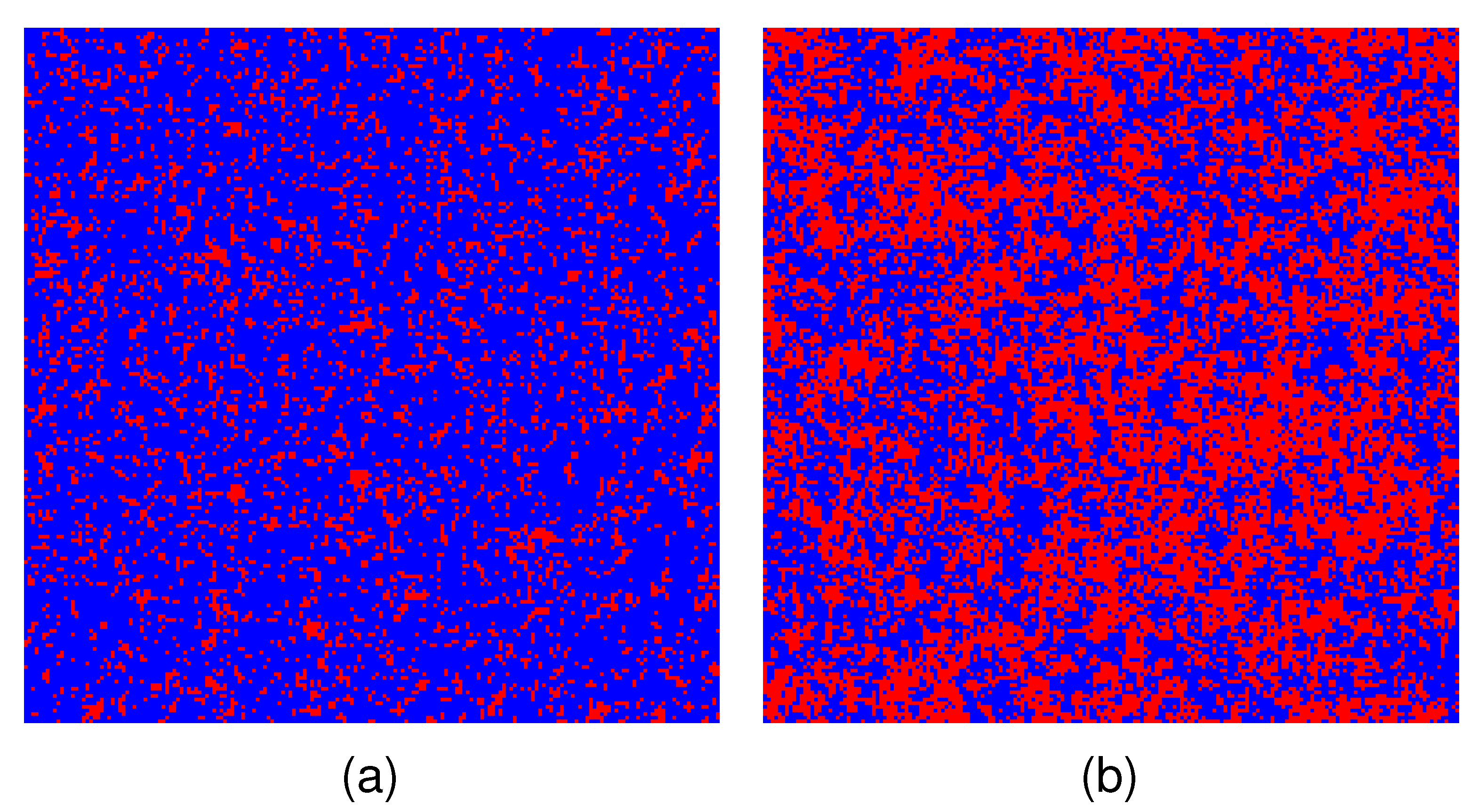However, as shown in Figure 9a, the geometric clusters defined on a 2D cross-section at $T_p^{3D}$ do not display self-similar scaling behavior, since the minority clusters are small, and a single majority cluster spans the slice. This shows that $T_p^{3D}$ is not the percolation point for 2D slice geometric clusters. On the other hand, inspired by the fact that the percolation point coincides with the critical point for 2D Ising model [28], we find that at $T_c^{3D}$, as shown by Figure 9b, the 2D cross-sectional geometric clusters indeed show self-similarity and fractal behavior over all lengthscales in the field of view. This is consistent with the findings of Ref. [34], which argues that $T_p^{\mathrm{slice}}=T_c^{3D}$. Additionally, our numerical simulation in Section 5 corroborates $T_p^{\mathrm{slice}}=T_c^{3D}$ from various perspectives, including robust power law behaviors of 2D slice geometric clusters at $T_c^{3D}$ and change of behavior of pair-connectivity function through $T_c^{3D}$.

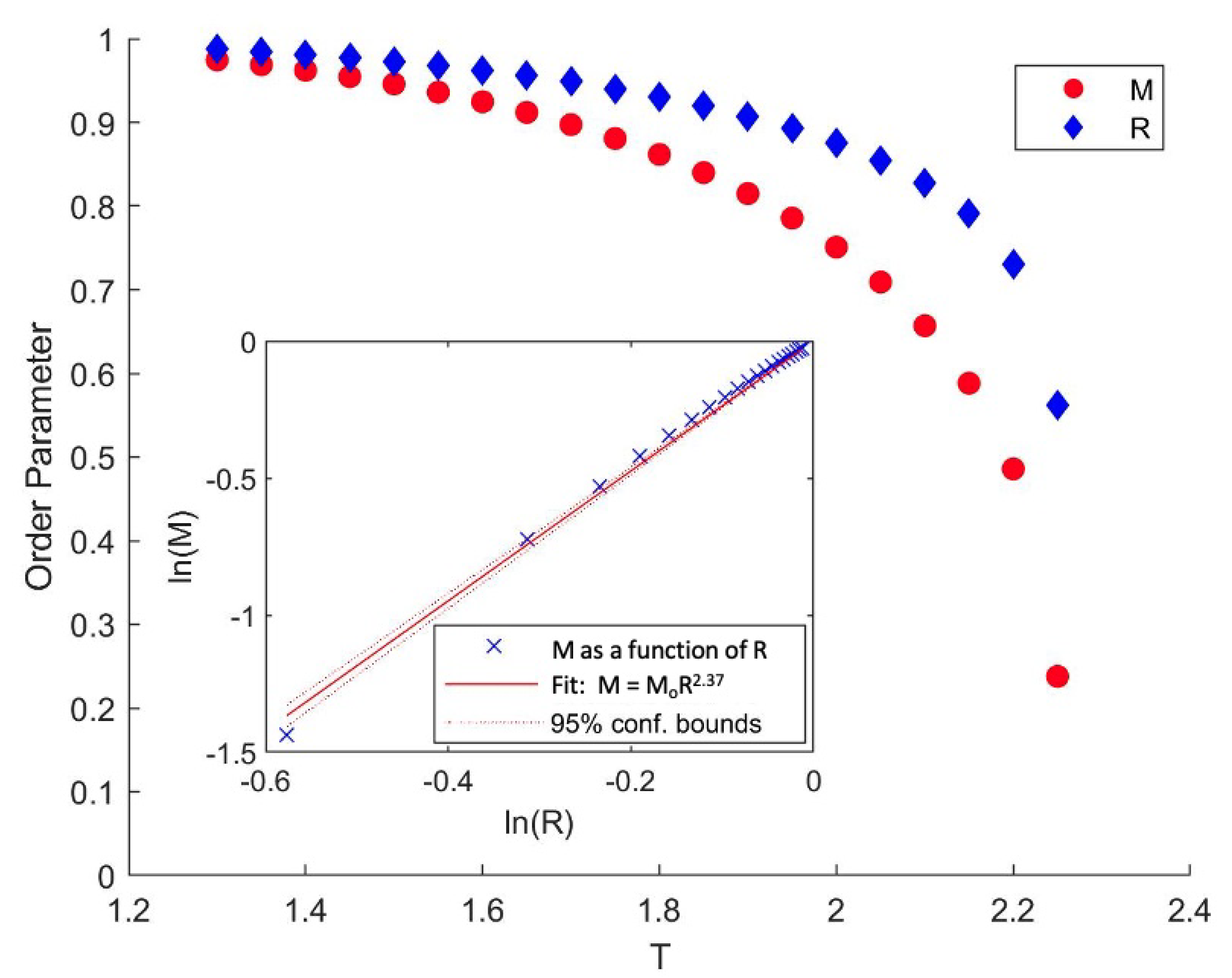
In the clean 2D Ising model, Coniglio and co-workers [28] showed that the percolation temperature coincides with the thermodynamic transition temperature, $T_p=T_c$, by showing that $M<R$, where M is the net magnetization and R is the infinite network strength, defined as the ratio of the number of sites in the infinite connected geometric cluster to the total number of sites in the system. This stems from the very physical idea that in a 2D system with thermal fluctuations, a net magnetization requires that at least one geometric cluster spans the system. From Figure 9, it appears that something similar must be going on in the 3D Ising model, when clusters are defined as a 2D slice. As will be discussed later in this section, our numerical results indeed show that $M<R^{slice}$, where $R^{slice}$ is the infinite network strength defined on a plane of a 3D system (Note that in Ref. [51], Coniglio et al. showed that $M<R$ in any dimension, for $T<Tc$. The question here is whether $M<R_x$ on a 2D slice in a 3D system).

To rigorously prove that $T_p^{\mathrm{slice}}=T_c^{3D}$ would require a proof the following lemma: For a 2D slice of the 3D ferromagnetic Ising model with nearest-neighbor interactions at zero external field ($H=0$) and below the critical temperature ($T<T_c$), we have

$$\begin{array}{c}\hfill M(0^{+},T)\le R_{\uparrow }^{slice}(0^{+},T)-R_{\downarrow }^{slice}(0^{+},T).\end{array}$$

(5)

The symbol $0^{+}$($0^{-}$) means $H=0$ with $(+)$-boundary ($(-)$-boundary) condition. For our discussion, we limit ourselves to the $(+)$-boundary by convention, and the results of $(-)$-boundary follow those of $(+)$-boundary under symmetry. $M(0^{+},T)$ is the reduced spontaneous magnetization on the 2D slice (which is identical to the reduced spontaneous magnetization of the bulk system at thermodynamic limit), and is given by $M(0^{+},T)={\langle {\tilde{\pi }}_0\rangle }_{+}-{\langle {\pi }_0\rangle }_{+}$. Here

$$\begin{array}{c}\hfill {\pi }_i=\frac{1}{2}(1-{\sigma }_i)\\ \hfill {\tilde{\pi }}_i=\frac{1}{2}(1+{\sigma }_i)\end{array}$$

(6)

are the lattice gas variables relative to the ith site, and ${\sigma }_i=\pm 1$ is the usual Ising spin variable. ${\tilde{\pi }}_i$ (${\pi }_i$) is equivalently the characteristic function of the event that spin i is up (down). The characterstic function of an event is that when the event happens, the function takes the value 1, otherwise it takes the value 0. The subscript 0 refers to the origin, and ${\langle \rangle }_{+}$ means the thermal average for the Ising model with $(+)$-boundary. Here we only take one slice for each Ising configuration to be counted in the thermal average, and we do not average over slices belonging to the same configuration in order to reduce spatial dependence. Therefore, there is a one-to-one correspondence between the slice configuration and bulk system configuration, and by convention we fix the slice to be the $z=0$ plane in the ${\mathbb{Z}}^3$ cubic lattice so that the slice contains the origin. $R_{\uparrow }^{slice}(0^{+},T)$($R_{\downarrow }^{slice}(0^{+},T)$) is the 2D slice infinite network strength for up(down) spins, defined as the probability that the origin belongs to the infinite 2D slice $(+)$-cluster ($(-)$-cluster), or equivalently, it is the weight of the infinite 2D slice $(+)$-cluster($(-)$-cluster). Mathematically, it is given by $R_{\uparrow }^{slice}(0^{+},T)={\langle {\tilde{\gamma }}_0^{\infty }\rangle }_{+}$ ($R_{\downarrow }^{slice}(0^{+},T)={\langle {\gamma }_0^{\infty }\rangle }_{+}$), where ${\tilde{\gamma }}_i^{\infty }$(${\gamma }_i^{\infty }$) is the characteristic function of the event that spin in i belongs to the infinite 2D slice $(+)$-cluster($(-)$-cluster).

For the 2D slice of a cubic lattice system, which is a simple planar graph admitting an elementary cell and two axes of symmetry, we have the statement that (i) an infinite 2D slice $(+)$-cluster cannot coexist with an infinite 2D slice $(-)$-cluster, and (ii) the number of each type of infinite 2D slice cluster must be either 0 or 1 [28,51,53,54,55]. This means that

$$\begin{array}{c}\hfill R_{\uparrow }^{slice}(H,T)R_{\downarrow }^{slice}(H,T)=0,\end{array}$$

(7)

and thus, there can only be at most one infinite $(+)$-cluster on the 2D slice with the $(+)$ boundary condition. While one can conceive of two infinite clusters which both span the system (i.e., skinny clusters which stretch from one side to the opposite side), the isotropy of the model ensures that the naturally occurring clusters are isotropic in the thermodynamic limit. Therefore, Equation (2) equivalently becomes

$$\begin{array}{c}\hfill M(0^{+},T)\le R_{\uparrow }^{slice}(0^{+},T),\end{array}$$

(8)

as intuitively discussed in the previous paragraph.

The rigorous demonstration of (4) requires that the Markov property [56] and the Fortuin–Kasteleyn–Ginibre (FKG) inequality [57] both hold [28]. The FKG inequality (the FKG inequality concerns the relation of the expectation value of the product of two functions of Ising variables to the product of the expectation values. See Refs. [28,57].) may be directly extended to the 2D slice since it is applicable to any finite set in the bulk system. However, the Markov property cannot be restricted to a 2D slice, since the Markov chain may extend off the slice in a 3D system. Rather than delving into a mathematical physics approach, for the purpose of this paper, we numerically demonstrate the fact that the inequality (4) holds for the 2D slice embedded in the 3D Ising model, as revealed by Figure 10.

By symmetry, we have $R_{\uparrow }^{slice}(H,T)=R_{\downarrow }^{slice}(-H,T)$. Therefore, from Equation (3), for $T\ge T_c^{3D}$, we must have $R_{\uparrow }^{slice}(0,T)=R_{\downarrow }^{slice}(0,T)=0$. For $T<T_c^{3D}$, Equations (3) and (4) yield $R_{\downarrow }^{slice}(0^{+},T)=0$ and $R_{\uparrow }^{slice}(0^{+},T)\ge M(0^{+},T)>0$. If we suppose that the finite cluster weight is continuous and has a limit at $T_c^{3D}$, then due to symmetry we have ${lim}_{T\to T_c^{3D}}{\langle {\tilde{\gamma }}_0\rangle }_{+}={lim}_{T\to T_c^{3D}}{\langle {\gamma }_0\rangle }_{+}$. From

$$\begin{array}{ccc}\hfill M(0^{+},T)& =& {\langle {\tilde{\pi }}_0\rangle }_{+}-{\langle {\pi }_0\rangle }_{+}\hfill \\ & =& {\langle {\tilde{\gamma }}_0\rangle }_{+}-{\langle {\gamma }_0\rangle }_{+}+{\langle {\tilde{\gamma }}_0^{\infty }\rangle }_{+}-{\langle {\gamma }_0^{\infty }\rangle }_{+},\hfill \end{array}$$

(9)

we have ${lim}_{T\to T_c^{3D}}{\langle {\tilde{\gamma }}_0^{\infty }\rangle }_{+}={lim}_{T\to T_c^{3D}}{\langle {\gamma }_0^{\infty }\rangle }_{+}$, which then leads to ${lim}_{T\to T_c^{3D}}{R}_{\uparrow }^{slice}(0^{+},T)=0$, so that no jump occurs at $T_c^{3D}$. This is intuitively consistent with a continuous phase transition. In other words, under the $(+)$ boundary condition with zero external field, the 2D slice $(+)$-cluster percolates at $T_c^{3D}$, as characterized by the percolation order parameter $R_{\uparrow }^{slice}(0^{+},T)$ which continuously changes from 0 to non-zero.

All of the above statements apply to the $(-)$-cluster with $(-)$ boundary condition under symmetry. Thus, for zero applied field $H=0$, the $(+)$-cluster and $(-)$-cluster defined on a 2D slice both approach the percolation point at the limit $T\to T_c^{3D}$. The spontaneous infinite cluster type in the ordered phase $T<T_c^{3D}$ is decided by the boundary condition (whether $(+)$ or $(-)$), and is symmetric under $H=0^{+}\leftrightarrow H=0^{-}$. Therefore, with $H=0$ at the limit $T\to T_c^{3D}$, both types of clusters percolate on the slice, and due to symmetry they present the same universal scaling behavior with the same critical exponents.

As supported by our numerical simulation as summarized in Table 3, this critical percolation point of geometric clusters defined on 2D slices of the bulk system in the 3D clean Ising model is a new universality class of geometric criticality, distinct from that of the clean 2D model and uncorrelated percolation in 2D, as well as that of the bulk percolation which occurs inside the ordered phase of the 3D system, since $T_p^{3D}\ne T_p^{\mathrm{slice}}$.

8. Two Correlation Lengths

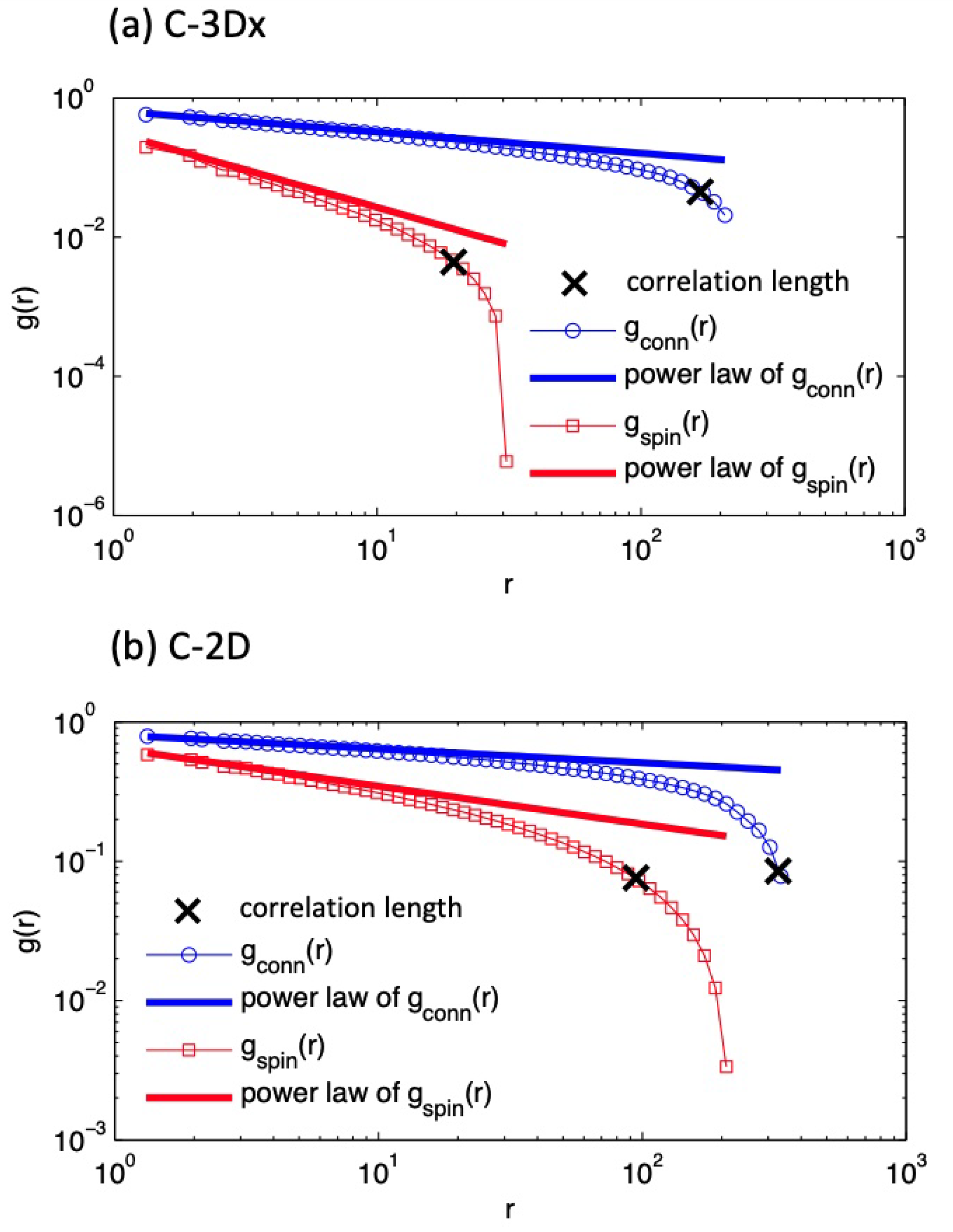
In this section we elaborate on the two different correlation lengths associated with the pair connectivity function and the spin-spin correlation function. In Figure 11, we show the pair connectivity function $g_{\mathrm{conn}}$ and spin-spin correlation function $g_{\mathrm{spin}}$ for both the 2D slice of the 3D clean Ising model and 2D clean Ising model near their respective transition temperatures with specific system sizes ($L=160$ for C-3Dx and $L=256$ for C-2D). The spin-spin correlation function is defined as

$$g_{\mathrm{spin}}\left(r\right)=〈{\sigma }_0{\sigma }_i〉-〈{\sigma }_0〉〈{\sigma }_i〉$$

(10)

where r is the distance between the origin and site i. Since $g_{\mathrm{spin}}$ approaches 0 for large r, it can fluctuate into negative values under our simulation with finite system sizes and finite number of configurations for averaging. Once negative values appear, in Figure 11 we cut off the remaining points with larger length scales on the log-log plots.

By doing scaling form fits of the correlation functions, we can extract the correlation length for each function. The scaling form that we fit for the pair connectivity function $g_{\mathrm{conn}}\left(r\right)$ is in Equation (4), which gives the correlation length ${\xi }_p$ of geometric criticality. We use the following scaling form fit for $g_{\mathrm{spin}}\left(r\right)$ near criticality:

$$g_{\mathrm{spin}}\sim r^{-(d-2+{\eta }_c)}{e}^{-r/{\xi }_c}$$

(11)

In Panel (a) of Figure 11, which is calculated at the thermodynamic critical temperature $T_c^{3D}(L\to \infty )$ of the infinite size system for C-3Dx, these two correlation lengths are ${\xi }_p=168\pm 4.9$ and ${\xi }_c=19.5\pm 0.6$, where the error bars are estimated from the standard deviation of the correlation lengths in the simulations from the critical form $\xi \propto {1/|T-Tc|}^{\nu }$ over the temperature range reported in Figure 12. In Panel (b) of Figure 11, which is calculated at thermodynamic critical temperature $T_c^{2D}(L\to \infty )$ of the infinite size system for C-2D, these correlation lengths are ${\xi }_p=327\pm 9.5$ and ${\xi }_c=95\pm 2.8$, where the error bars are once again estimated from the standard deviation of the correlation lengths in the simulations from the critical form $\xi \propto {1/|T-Tc|}^{\nu }$ over the temperature range reported in Figure 12. Note that in both cases, ${\xi }_p$ extracted by this method has exceeded the system size, and is subject to finite size effects. In addition, these graphs should be considered to be near but not at criticality, since finite size effects lower the transition temperature from the bulk value. Nevertheless, in both cases, ${\xi }_p$ is much larger than ${\xi }_c$. From the scaling form fits, we have $d-2+{\eta }_c=1.078\pm 0.068$ for C-3Dx, and $d-2+{\eta }_c=0.272\pm 0.008$ for C-2D. They are very close to the established values $d-2+{\eta }_c=1.0336$ [58] and $d-2+{\eta }_c=0.25$ [38,59], respectively, corroborating the validity of our results for the spin-spin correlation lengths. The results for $d-2+{\eta }_p$ from the fits are already reflected in the insets (a) of Figure 5 and Figure 7.

As implied in our previous discussion, these two different correlation lengths correspond to two categories of criticality, geometric criticality (${\xi }_p$) and thermodynamic criticality (${\xi }_c$), with two distinct order parameters (the infinite network strength R and the magnetization M, respectively). For C-2D, it is well established that the correlation length exponents ${\nu }_p$ (based on geometric clusters) and ${\nu }_c$ (based on FK clusters) are different and are related by ${\nu }_p\ge {\nu }_c$ [28]. Therefore, near the critical point $T_p^{2D}=T_c^{2D}$, from the relation $\xi \sim |T-T_c{|}^{-\nu }$, the connectivity correlation length of geometric clusters is expected to be large compared to the spin-spin correlation length (${\xi }_p>{\xi }_c$). This is consistent with our simulation Figure 11b. Our simulation Figure 11a reveals that ${\xi }_p>{\xi }_c$ also applies for C-3Dx.

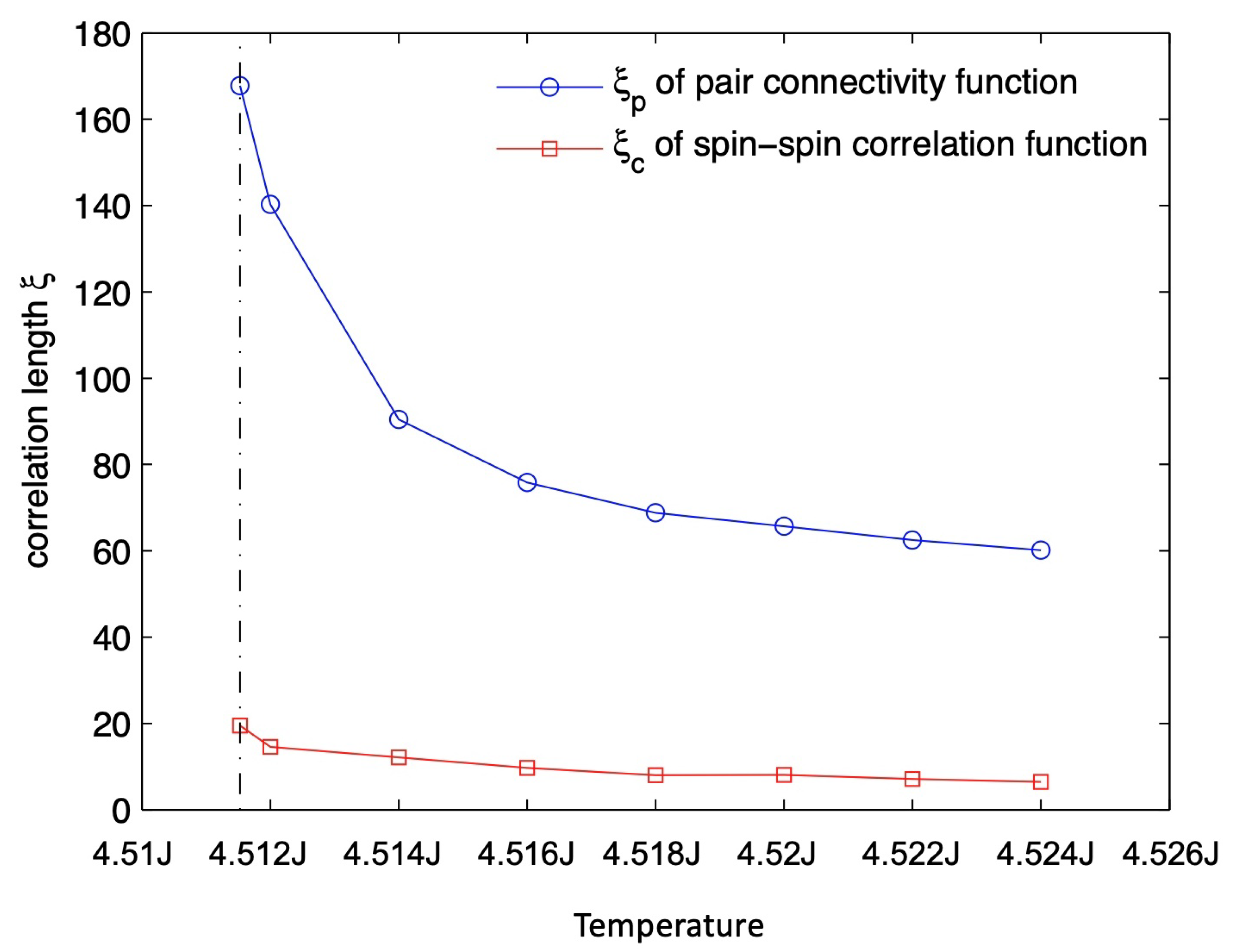
To further validate this inequality, in Figure 12, we compute the two correlation lengths for C-3Dx geometric criticality as a function of temperature near the critical point $T_p^{slice}=T_c^{3D}$ on the disordered side, where the correlation function is consistent with the scaling form shape. As shown by Figure 12, ${\xi }_p$ is always much larger than ${\xi }_c$, and they increase as $T\to T_c$. This suggests that the exponent inequality ${\nu }_p\ge {\nu }_c$ also applies for C-3Dx.

9. Discussion

So far, we have argued that the bulk thermodynamic critical point of the 3D clean Ising model coincides with the percolation of geometric clusters defined on a 2D slice, $T_p^{slice}=T_c^{3D}$. Furthermore, we have numerically investigate this geometric criticality by extracting the critical cluster exponents and studying the behaviors of the pair-connectivity functions (together with the 2D clean Ising model). These results have several important implications:

(1) There are two length scales in the clean 3D Ising model. Aside from the usual length scale associated with the spin-spin correlation length ${\xi }_c$, we have defined a new length scale, ${\xi }_p$, which is the correlation length of the pair connectivity function of geometric clusters defined on a 2D slice. We have furthermore shown that these two length scales diverge differently as $T\to T_c^{3D}$, and that the generic case is that ${\xi }_p>{\xi }_c$. One consequence of this is that near this critical point, experiments which can detect clusters on a slice (for example, scanning probes like scanning tunneling microscopy) should reveal that the pair connectivity function defined on a slice is power law over a larger region of the phase diagram than the spin-spin correlation function. That is, the critical region appears to be larger when measured via a pair correlation function than via a spin-spin correlation function. The argument above also applies to the 2D clean Ising model.

(2) As discussed in the context of Conjecture #2 in Section 4, for the 2D clean Ising model, the geometric cluster percolation exponents and thermodynamic critical exponents are different in definition and values, but they satisfy the same scaling relation in their own respective closed sets. As in the purely 2D case, there are also two distinct sets of critical exponents at $T_c^{3D}$ for the clean 3D Ising model. One set comes from the geometric clusters defined on a 2D slice of the clean 3D Ising system, and the other from the bulk FK clusters. Using the numerical values derived in this work, the scaling relation $d-2+\eta =2(d-d_v)$ is satisfied within error bars. Inserting the values from Table 3, $d-2+{\eta }_p=0.322\pm 0.002$, and $d_{v,p}=1.856\pm 0.018$ gives $2(d-d_{v,p})=0.288\pm 0.036$. The scaling relation $\tau =(d+d_v)/d_v$ is almost satisfied: From the Table, we have $\tau =2.001\pm 0.013$ and $d_{v,p}=1.856\pm 0.018$, so that $(d+d_{v,p})/d_{v,p}=2.078\pm 0.010$. Recall that the scaling function associated with the exponent $\tau$ suffers from a significant scaling bump, which skews the value of $\tau$ to lower values in finite size systems. The slight mismatch in this scaling relation is likely due to this well-known finite size effect for $\tau$ [42].

We find some indication that the Coniglio inequalities for these two different sets of critical exponents also hold on a 2D slice of the 3D clean Ising model. For example, our results in Figure 12 suggest that the exponent inequality derived by Coniglio and coworkers [28] for the correlation length exponents ${\nu }_p$ and ${\nu }_c$ at the C-2D critical point also holds at the C-3Dx critical point, ${\nu }_p\ge {\nu }_c$.

(3) The C-3Dx fixed point represents a new universality class: not only are the critical exponents numerically distinct from the geometric criticality of the 2D clean Ising system and from 2D uncorrelated percolation, but they are also distinct from the values of bulk percolation in the 3D clean Ising model, which happens inside the ordered phase $T_p^{3D}<T_c^{3D}=T_p^{\mathrm{slice}}$.

(4) All of the above implies that there are two order parameters on the 2D slice of the 3D clean Ising model, just as there are two order parameters in the 2D clean Ising model. One of them is associated with the thermodynamic phase transition, and the other is associated with the geometric cluster percolation.

10. Conclusions and Outlook

In summary, we have studied geometric criticality associated with the correlated percolation of interacting geometric clusters on a 2D slice of clean 3D Ising models (C-3Dx). We find that as in the clean 2D Ising model (C-2D), the geometric criticality associated with the percolation of interacting geometric clusters at the C-3Dx critical fixed point corresponds to a unique geometric universality class which is distinct from that of uncorrelated percolation.

In addition, we find that at both the C-3Dx fixed point and the C-2D fixed point, the geometric clusters become fractal, meaning they acquire self-similar spatial structure leading to fractal hull and volume dimensions, and leading to power law behavior in the pair connectivity function. We find that in the vicinity of thermodynamic criticality, the pair connectivity function displays power law behavior over a wider region of the phase diagram than does the spin-spin correlation function.

One consequence of this finding is that the pair connectivity function can be a useful tool for diagnosing criticality in the context of image data from probes which can take “slice” data, as well as potentially from scanning surface image probes such as scanning tunneling microscopy, atomic force microscopy, and scanning infrared microscopy. In a future publication, we will explore the relation of these concepts to surface criticality, which is relevant for the application of these ideas to scanning surface probes. Especially in light of the tremendous increase in data coming from a growing number of scanning image probes [2], it is useful to have another method of analysis in hand. We expect that future studies regarding geometric criticality in random bond and random field Ising models will further facilitate the application of geometric cluster analyses to the interpretation of the many types of 2D image probe experimental techniques, especially in cases where complex pattern formation is observed [14,15,16,25].