Article

Dynamical Thermalization of Interacting Fermionic Atoms in a Sinai Oscillator Trap

by
Klaus M. Frahm
1,
Leonardo Ermann
2 and
Dima L. Shepelyansky
1,*
1
Laboratoire de Physique Théorique, IRSAMC, Université de Toulouse, CNRS, UPS, 31062 Toulouse, France
2
Departamento de Física Teórica, GIyA, Comisión Nacional de Energía Atómica, CP1650 Buenos Aires, Argentina
*
Author to whom correspondence should be addressed.
Condens. Matter 2019, 4(3), 76; https://doi.org/10.3390/condmat4030076
Submission received: 15 July 2019 / Revised: 3 August 2019 / Accepted: 6 August 2019 / Published: 8 August 2019
(This article belongs to the Special Issue Many Body Quantum Chaos)

Abstract

:
We study numerically the problem of dynamical thermalization of interacting cold fermionic atoms placed in an isolated Sinai oscillator trap. This system is characterized by a quantum chaos regime for one-particle dynamics. We show that, for a many-body system of cold atoms, the interactions, with a strength above a certain quantum chaos border given by the Åberg criterion, lead to the Fermi–Dirac distribution and relaxation of many-body initial states to the thermalized state in the absence of any contact with a thermostate. We discuss the properties of this dynamical thermalization and its links with the Loschmidt–Boltzmann dispute.

1. Introduction

The problem of emergence of thermalization in dynamical systems started from the Loschmidt–Boltzmann dispute about time reversibility and thermalization in an isolated system of moving and colliding classical atoms [1,2] (see the modern overview in [3,4]). The modern resolution of this dispute is related to the phenomenon of dynamical chaos where an exponential instability of motion breaks the time reversibility at infinitely small perturbation (see e.g., [5,6,7,8]). The well known example of such a chaotic system is the Sinai billiard in which a particle moves inside a square box with an internal circle colliding elastically with all boundaries [9].
The properties of one-particle quantum systems, which are chaotic in the classical limit, have been extensively studied in the field of quantum chaos during the last few decades and their properties have been mainly understood (see, e.g., [10,11,12]). Thus, it was shown that the level spacing statistics in the regime of quantum chaos [13] is the same as for Random Matrix Theory (RMT) invented by Wigner for a description of spectra of complex nuclei [14,15]. This result became known as the Bohigas–Giannoni–Schmit conjecture [13,16]. Thus, classically chaotic systems ( e.g., Sinai billiard) are usually characterized by Wigner–Dyson (RMT) statistics with level repulsion [13,14,15] while the classically integrable systems usually show Poisson statistics for level spacing distribution [11,12,16]. In this way, the level spacing statistics gives a direct indication for ergodicity (Wigner–Dyson statistics) or non-ergodicity (Poisson statistics) of quantum eigenstates. It was also established that the classical chaotic diffusion can be suppressed by quantum interference effects leading to an exponential localization of eigenstates [17,18,19,20] being similar to the Anderson localization in disordered solid-state systems [21]. The localized phase is characterized by Poisson statistics and the delocalized or metallic phase has RMT statistics. For billiard systems, the localized (nonergodic) and delocalized (ergodic) regimes appear in the case of rough billiards as described in [22,23].
It was also shown that, in the regime of quantum chaos, the Bohr correspondence principle [24] and the fully correct semiclassical description of quantum evolution remain valid only for a logarithmically short Ehrenfest time scale t E ln ( 1 / ) / h [17,19]. Here, is an effective dimensionless Planck constant and h in the Kolmogorov–Sinai entropy characterizing the exponential divergence of classical trajectories. This result is in agreement with the Ehrenfest theorem, which states that the classical-quantum correspondence works on a time scale during which the wave packet remains compact [25]. However, for the classically chaotic systems, the Ehrenfest time scale is rather short due to an exponential instability of classical trajectories. After the Ehrenfest time scale t E , the quantum out-of-time correlations (or OTOC as it is used to say now) stop decaying exponentially in contrast to exponentially decaying classical correlators [26,27]. For t > t E , the decay of quantum correlations stops and they remain on the level of quantum fluctuations being proportional to [26,27,28]. Since the level of quantum fluctuations is proportional to , the classical diffusive spreading over the momentum is affected by quantum corrections only on a significantly larger diffusive time scale t D 1 / 2 t E ln ( 1 / ) [17,19,26,27,28].
The problem of the emergence of RMT statistics and quantum ergodicity in many-body quantum systems is more complex and intricate as compared to one-particle quantum chaos. Indeed, it is well known that, in many-body quantum systems, the level spacing between nearest energy levels drops exponentially with the increase of number of particles or with energy excitation δ E above the Fermi level in finite size Fermi systems, e.g., in nuclei [29]. Thus, at first glance, it seems that an exponentially small interaction between fermions should mix many-body quantum levels leading to RMT level spacing statistics (see, e.g., [30]).
Furthermore, the size of the Hamiltonian matrix of a many-body system grows exponentially with the number of particles, but, since all interactions have a two-body nature, the number of nonzero interaction elements in this matrix does not grow faster than the number of particles in the fourth power. Thus, we have a very sparse matrix being rather far from the RMT type. A two-body random interaction model (TBRIM) was proposed in [31,32] to consider the case of generic random two-body interactions of fermions in the limiting case of strong interactions when one-particle orbital energies are neglected. Even if the TBRIM matrix is very sparse, it was shown that the level spacing statistics p ( s ) is described by the Wigner–Dyson or RMT distribution [33,34].
However, it is also important to analyze another limiting case when the two-body interaction matrix elements of strength U are weak or comparable with one-particle energies with an average level spacing Δ 1 . In metallic quantum dots, this case with U / Δ 1 1 / g corresponds to a large conductance of a dot g = E T h / Δ 1 1 , where E T h = / t D is the Thouless energy with t D being a diffusion spread time over the dot [35,36,37]. In this case, the main question is about critical interaction strength U or excitation energy δ E above the Fermi level of the dot at which the RMT statistics becomes valid. First, numerical results and simple estimates for a critical interaction strength in a model similar to TBRIM were obtained by Sven Åberg in [38,39]. The estimate of a critical interaction U c , called the Åberg criterion [40], compares the typical two-body matrix elements with the energy level spacing Δ c between quantum states directly coupled by two-body interactions. Thus, the Åberg criterion tells that the Poisson statistics is valid for many-body energy levels for U < U c Δ c and the RMT statistics sets in for U > U c Δ c . In [41], this criterion, proposed independently of [38,39], was applied to the TBRIM of weakly interacting fermions in a metallic quantum dot being confirmed by extensive numerical simulations. It was also argued that the dynamical thermalization sets in an isolated finite fermionic system for energy excitations δ E above the critical border δ E c h determined from the above criterion [41]:
δ E > δ E c h g 2 / 3 Δ 1 , g = Δ 1 / U .
The emergence of thermalization in an isolated many-body system induced by interactions between particles without any contact with an external thermostat represents the Dynamical Thermalization Conjecture (DTC) proposed in [41]. The validity of the Åberg criterion was numerically confirmed for various physical models (see [40] and references therein). An additional confirmation was given by the analytical derivation presented in [42] showing that, for three interacting particles, in a metallic dot the RMT sets in when the two-body matrix elements U become larger than the two-particle level spacing Δ 2 Δ c being parametrically larger than the three-particle level spacing Δ 3 Δ 2 . The advanced theoretical arguments developed in [43,44] confirm the relation (1) for interacting fermions in a metallic quantum dot.
The test for the transition from Poisson to RMT statistics is rather direct and needs only the knowledge of energies’ eigenvalues. However, the verification of DTC is much more involved since it requires the computation of system eigenstates. Thus, it is much more difficult to check numerically the relation (1) for DTC. However, it is possible to show that there is a transition from non-thermalized eigenstates at weak interactions (presumably for δ E < δ E c h ) to dynamically thermalized individual eigenstates at relatively strong interactions (presumably for δ E > δ E c h ). Thus, for the TBRIM with fermions, the validity of DTC for individual eigenstates at U > U c Δ c has been demonstrated in [45,46] by the computation of energy E and entropy S of each eigenstate and its comparison with the theoretical result given by the Fermi–Dirac thermal distribution [47].
Even if the TBRIM represents a useful system for DTC tests, it is not so easy to realize it in real experiments. Thus, in this work, we investigate the DTC features in a system of cold fermionic atoms placed in the Sinai oscillator trap created by a harmonic two-dimensional potential with a repulsive circular potential created by a laser beam in a vicinity of the trap center. In such a case, the repulsive potential in the center is modeled as an elastic circle as in the case of Sinai billiard [9]. For one particle, it has been shown in [48] that the Sinai oscillator has an almost fully chaotic phase space and that, in the quantum case, the level spacing statistics is described by the RMT distribution. Due to one-particle quantum chaos in the Sinai oscillator, we expect that this system will have properties similar to the TBRIM. On the other side, the Sinai oscillator trap has been already experimentally realized with Bose–Einstein condensate of cold bosonic atoms [49,50,51]. At present, cold atom techniques allow for investigating various properties of cold interacting fermionic atoms [52,53] and we argue that the investigation of dynamical thermalization of such fermionic atoms, e.g., 6 L i , in a Sinai oscillator trap is now experimentally possible. Thus, in this work, we study properties of DTC of interacting fermionic atoms in a Sinai oscillator trap. Here, we consider the two-dimensional (2D) case of such a system assuming that the trap frequency in the third direction is small and that the 2D dynamics are not significantly affected by the adiabatically slow motion in the third dimension.
Finally, we note that, at present, the TBRIM model in the limit of strong interactions attracts a high interest in the context of field theory since, in this limit, it can be mapped on a black hole model of quantum gravity in 1 + 1 dimensions known as the Sachdev–Ye–Kitaev (SYK) model linked also to a strange metal [54,55,56,57,58,59]. In fact, the SYK model, in its fermionic formulation [56], corresponds to the TBRIM considered with a conductance close to zero g 0 . In these lines, the dynamical thermalization in TBRIM and SYK systems has been discussed in [45,46]. Furthermore, there is also a growing interest in dynamical thermalization for various many-body systems known also as the eigenstate thermalization hypothesis (ETH) and many-body localization (MBL) (see, e.g., [60,61,62,63]). We think that the system of interacting fermionic atoms in a Sinai oscillator trap captures certain features of TBRIM and SYK models and thus represents an interesting test ground to investigate nontrivial physics of these systems in real cold atom experiments.
This paper is composed as follows: in Section 2, we describe the properties of the one-particle dynamics in a Sinai oscillator; numerical results for dynamical thermalization on interacting atoms in this oscillator are presented in Section 3; the conditions of thermalization for fermionic cold atoms in realistic experiments are given in Section 4; the discussion of the results is presented in Section 5.

2. Quantum Chaos in Sinai Oscillator

The model of one particle in the 2D Sinai oscillator is described in detail in [48] with the Hamiltonian:
H 1 = 1 2 m ( p x 2 + p y 2 ) + m 2 ( ω x 2 x 2 + ω y 2 y 2 ) + V d ( x , y ) .
Here, the first two terms describe the 2D oscillator with frequencies ω x , ω y and the last term gives the potential wall of elastic disk of radius r d . We choose the dimensionless units with mass m = 1 , frequencies ω x = 1 , ω y = 2 and disk radius r d = 1 . The disk center is located at ( x d , y d ) = ( 1 / 2 , 1 / 2 ) so that the disk bungs a hole in the center as it was the case in the experiments [49]. The Poincare sections at different energies are presented in [48] showing that the phase space is almost fully chaotic (see Figure 1 there). The quantum evolution is described by the Schrödinger equation with the quantized Hamiltonian (2), where the conjugate momentum and coordinate variables become operators with the commutation relation [ x , p x ] = [ y , p y ] = i [48]. For the quantum problem, we use the value of the dimensionless Planck constant = 1 so that the ground state energy is E g = 1.685 . In the following, the energies are expressed in atomic like units of energy E u = ω x (for our choice of Sinai oscillator parameters, we also have E u = ω x = 2 / ( m r d 2 ) ) [48] with the typical size of oscillator ground state being equal to the disk radius: a 0 = Δ x o s c = ( / m ω x ) 1 / 2 = r d .
In [48], it is shown that the classical dynamics of this system are almost fully chaotic. In the quantum case, the level spacing statistics is well described by the RMT distribution. The average dependence of energy level number k is well described by the theoretical dependence k ( ε ) = ε 2 / ( 2 2 ) ε / 2 [48]. Thus, the one-particle density of states ρ 1 ( ε ) and corresponding level spacing Δ 1 are:
ρ 1 ( ε ) = d k d ε = ε 2 1 2 , Δ 1 = 1 ρ 2 ε 0.84 k .
Examples of several eigenstates, computed on a numerical grid of 28,341 spatial points, are shown in Figure 1. More details on the numerical diagonalization of (2) and other example eigenstates can be found in [48].

3. Sinai Oscillator with Interacting Fermionic Atoms

3.1. Two-Body Interactions of Fermionic Atoms

The two-body interaction of atoms appears usually due to van der Waals forces which drop rapidly with the distance between two atoms and the short ranged interaction can be described in the framework of the scattering length approach (see, e.g., [64,65]). Therefore, we assume that the finite effective interaction range r c is significantly smaller than the disk radius r d and the typical size of the wave function, i.e., r c r d . Such a short range interaction is indeed used to modelize atomic interactions in harmonic traps (see, e.g., [66]). For example, in a typical experimental situation, the disk radius is of the order of micron r d 1 μ m = 10 4 cm, while, for Li and other alkali atoms, we have r c 3 × 10 7 cm [64,65]. Of course, in the limit of small r c r d , the interaction between two atoms takes place mainly in the s-wave scattering, so effectively the interaction operates between fermions with different quantum numbers of the Sinai oscillator. This feature is of course taken into account in our numerical simulations.
In the following, we use a simple interaction function having a constant amplitude U for r r c and being zero for r > r c , where we simply choose r c = 0.2 r d , which corresponds well to the short range interaction regime. The precise value of r c is not very important since a slight modification r c r ¯ c can be absorbed in a modified amplitude according to U U ¯ = U ( r ¯ c / r c ) 2 , a relation we verified numerically for various values of r ¯ c < r d . We numerically checked that, at a used r c = 0.2 r d value, we are in the regime when the interaction matrix elements are proportional to r c 2 so that we are in the regime of short-range interactions. We mention that, in experiments, the strength of the interaction amplitude can be changed by a variation of the magnetic field via the Feshbach resonance [67].

3.2. Reduction to TBRIM Like Case and Its Analysis

Using the methods described in [48], we numerically compute a certain number of one-particle or orbital energy eigenvalues ε k and corresponding eigenstates φ k ( r ) of the Sinai oscillator (2). As repulsive interaction potential v ( r ) , we choose the short ranged box function v ( r ) = U if | r | r c = 0.2 (since r d = 1 ) and v ( r ) = 0 , otherwise. Here, the parameter U > 0 gives the overall scale of the interaction strength depending on the charge of the particles and eventually other physical parameters.
Therefore, the corresponding many-body Hamiltonian with M one-particle orbitals and 0 L M spinless fermions takes the form:
H = k = 1 M ε k c k c k + i < j , k < l V i j , k l c i c j c l c k ,
where, for i < j and k < l , we have the interaction matrix elements:
V i j , k l = V ¯ i j , k l V ¯ i j , l k , V ¯ i j , k l = d r 1 d r 2 φ i * ( r 1 ) φ j * ( r 2 ) v ( r 1 r 2 ) φ k ( r 1 ) φ l ( r 2 )
and c k , c k are fermion operators for the M orbitals satisfying the usual anticommutation relations. We note that, in the literature, when expressing a two-body interaction potential in second quantization, one usually uses the raw matrix elements V ¯ i j , k l with an additional prefactor of 1 / 2 and full independent sums for the four indices i, j, k and l. Using the particle exchange symmetry: V ¯ i j , k l = V ¯ j i , l k , one can reduce the i , j sums to i < j , which removes the prefactor 1 / 2 (after exchanging the index names l and k for the i > j contributions and exploiting that contributions at i = j or l = k obviously vanish). The definition of the anti-symmetrized interaction matrix elements V i j , k l according to (5) allows for also reducing the k , l sums to k < l . Furthermore, the ordering of the two fermion operators c l c k in (4) is also important and necessary to obtain positive expectation values if the interaction is repulsive. The anti-symmetrized matrix elements V i j , k l correspond to a M 2 × M 2 matrix with M 2 = M ( M 1 ) / 2 ) . In order to avoid a global shift of the non-interacting eigenvalue spectrum due to the interaction, we also apply a diagonal shift V i j , i j V i j , i j ( 1 / M 2 ) k < l V k l , k l to ensure that this matrix has a vanishing trace ( One can easily show that the trace of the M 2 × M 2 anti-symmetrized interaction matrix is proportional to the trace of the interaction operator in the many-body Hilbert space with a factor depending on M and L). Of course, such a global energy shift does not affect the issues of thermalization, interaction induced eigenfunction mixing or the quantum time evolution with respect to the Hamiltonian H, etc.
We note that the transition from the classical Hamiltonian (2) to the quantum one (4) is done by the standard procedure of second quantization (see, e.g., [68]).

3.3. Aberg Parameter

In absence of interaction, the energy eigenvalues of (4) are given as the sum of occupied orbital energies:
E ( { n k } ) = k = 1 M ε k n k ,
where { n k } represents a configuration such that n k { 0 , 1 } and k n k = L . The associated eigenstates are the basis states where each orbital is either occupied (if n k = 1 ) or unoccupied (if n k = 0 ) and, in this work, we will denote these states in the usual occupation number representation: | n M n 2 n 1 > , where, for convenience, we write the lower index orbitals starting from the right side.
The distribution of the total one-particle energies (6) is numerically rather close to a Gaussian (since n k act as quasi-random numbers) with mean and variance (see also Equation (A.4) of Ref. [46]):
E mean = L ε ¯ , σ 0 2 = L ( M L ) M 1 ε 2 ¯ ε ¯ 2 , ε n ¯ = 1 M k = 1 M ε k n , n = 1 , 2 .
Therefore, the many-body level spacing Δ MB or inverse Heisenberg time at the band center E = E mean is given by Δ MB = 1 / t H = 2 π ( σ 0 / d ) , where d = M ! / ( L ! ( M L ) ! ) is the dimension of the fermion Hilbert space in the sector of M orbitals and L particles. In our numerical computations, we simply evaluated the quantities ε n ¯ of (7) using the exact one-particle energy eigenvalues obtained from the numerical diagonalization of the one-particle Sinai Hamiltonian H 1 given in (2). However, to get some analytical simplification for large M, one may use the one-particle density of states (3), which gives, after replacing the sums by integrals and neglecting the constant term, ε n ¯ 2 ε M n / ( n + 2 ) and ε 2 ¯ ε ¯ 2 ε M 2 / 18 2 M / 9 .
For the question of whether the interaction strength is sufficiently strong to mix the non-interacting basis states, the important quantity is the effective level spacing of states coupled directly by the interaction Δ c = 2 π [ σ 0 ( L = 2 ) / K ] , where K = 1 + L ( M L ) + L ( L 1 ) ( M L ) ( M L 1 ) / 4 is the number of nonzero elements for a column (or row) of H [41,69] and we need to use the variance for only two particles:
σ 0 2 ( L = 2 ) = 2 ( M 2 ) M 1 ε 2 ¯ ε ¯ 2 σ 0 2 ( L = 2 ) σ 0 2 = 2 ( M 2 ) L ( M L )
because the interaction only couples states where (at least) L 2 particles are on the same orbital such that (at most) only the partial sum of two one-particle energies is different between two coupled states. Even though for two particles the hypothesis of a Gaussian distribution is theoretically not justified, the distribution is still sufficiently similar to a Gaussian and it turns out that the value of 1 / Δ c = K / [ 2 π σ 0 ( L = 2 ) ] as the coupled two-particle density of states in the band center is numerically quite accurate with an error below 10% (for M = 16 and our choice of ε k values).
According to the Åberg criterion [38,39,41], the onset of chaotic mixing happens for typical interaction matrix elements U comparable to Δ c . Therefore, we compute the quantity V mean = | V i j , k l | 2 (which is proportional to the interaction amplitude U) where the average is done with respect to all M 2 2 matrix elements of the interaction matrix. This quantity might be problematic and not correspond to a typical interaction matrix element in the case of a long tail distribution. However, in our case, it turns out that V mean 2 exp ( ln | V i j , k l | ) , which excludes this scenario. Using this quantity, we introduce the dimensionless Åberg parameter and the critical interaction amplitude U c by A = V mean / Δ c = U / U c such that A = 1 if U = U c . We expect [38,39,41] to be the onset of strong/chaotic mixing at A 1 and a perturbative regime for A 1 , while, at A = 1 , we have the critical interaction strength U = U c . The value of U c depends on the parameters L, M, σ 0 and the overlap of the one-particle eigenstates according to (5). To obtain some useful analytical expression of U c , we note that the quantity V mean , numerically computed for 4 M 30 , can be quite accurately fitted by V mean 3 × 10 4 U / ε M . Furthermore, we remind readers of the expression Δ c = ( 1 / K ) 4 π ( M 2 ) ( ε 2 ¯ ε ¯ 2 ) / ( M 1 ) , which can be simplified in the limit M 1 and L 1 , such that K ( M L ) 2 L 2 / 4 , resulting in: Δ c = 4 / 3 2 π ε M / [ ( M L ) 2 L 2 ] . Here, we also used the found expression above ε 2 ¯ ε ¯ 2 ε M 2 / 18 . From this, we find that U c = Δ c U / V mean C M / [ ( M L ) 2 L 2 ] with a numerical constant C 16 × 10 4 π / 9 3.15 × 10 4 , where we also used ε M 2 2 2 M according to (3). Below, we will give more accurate numerical values of V mean , Δ c and U c for the parameter choice of M and L numerically relevant in this work.
We note that this estimate for A = U / U c applies to energies close to the many body band center of H and that, for energies away from the band center, the value of Δ c is enhanced, thus reducing the effective value of A. Furthermore, we computed V mean by a simplified average over all interacting matrix elements not taking into account an eventual energy dependence according to the index values of i , j , k , l in (5).

3.4. Density of States

In this work, we present numerical results for the case of M = 16 orbitals and L = 7 particles corresponding to a many-body Hilbert space of dimension d = M ! / ( L ! ( M L ) ! ) = 11440 and the number K = 820 of directly coupled states of a given initial state by non-vanishing interaction matrix elements in (4). Thus, in our studies, the whole Hilbert space is built only on these M = 16 orbitals. We diagonalize numerically the many-body Hamiltonian (4) for various values of A in the range 0.025 A 200 . We have also verified that the results and their physical interpretation are similar for smaller cases such as M = 12 , L = 5 (with d = 792 , K = 246 ) or M = 14 , L = 6 ( d = 3003 , K = 469 ).
We mention that, for M = 16 and L = 7 , we find numerically that V mean = 3.865 × 10 5 U and, from (8), that Δ c = 2 π [ σ 0 ( L = 2 ) / K ] = 6.1706 × 10 3 , where the quantities ε n ¯ were exactly computed from the numerical orbitals energies ε k . From this, we find that U c = Δ c U / V mean 159.65 . This expression is more accurate than the more general analytical estimate for arbitrary M 1 and L 1 given in the last section (which would provide U c 127 for M = 16 and L = 7 ).
Our first observation is that, even in the presence of interactions, the density of states has approximately a Gaussian form with the same center E mean given in (7) for the case A = 0 . This is simply due the fact that the interaction matrix has, by choice, a vanishing trace and does not provide a global shift of the spectrum. We determine the variance σ 2 ( A ) of the Gaussian density of states by a fit of the integrated density of states P ( E ) using
P ( E ) = ( 1 + erf [ q ( E ) ] ) / 2 , q ( E ) = ( E E mean ) / [ 2 σ ( A ) ] ,
such that P ( E ) is a Gaussian of width σ ( A ) and center E mean (see Appendix A of Ref. [
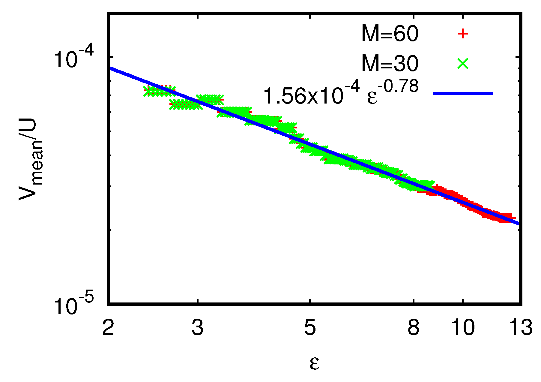
46] for more details). From this, we find the behavior:
σ 2 ( A ) = σ 0 2 ( 1 + α A 2 ) ,
where α is a constant depending on M and L; for M = 16 , L = 7 the fit values of σ 0 and α are σ 0 = 3.013 ± 0.009 and α = 0.00877 ± 0.00010 . It is also possible to determine σ ( A ) using the expression σ 2 ( A ) = T r Fock [ ( H E mean 1 ) 2 ] / d where the trace in Fock space can be evaluated either by using the matrix H before diagonalizing it or using its exact energy eigenvalues E m . This provides the same behavior as (10) with the very similar numerical values σ 0 = 3.013 ± 0.007 and α = 0.00858 ± 0.00008 (for M = 16 , L = 7 ). We mention that the integrated Gaussian density of states (9) is not absolutely exact but quite accurate for values A 10 . For larger values of A, the deviations increase, but the overall form is still correct. As described in [46], the quality of the fit can be considerably improved if we replace in (9) the linear function q ( E ) by a polynomial of degree 5. In this case, the precision of the fit is highly accurate for the full range of A values we consider. In particular, we use this improved fit to perform the spectral unfolding when computing the nearest level spacing distribution (shown below).
To obtain some theoretical understanding of (10), one can consider a model where the initial interaction matrix elements (5) are replaced by independent Gaussian variables with identical variance V mean 2 . In this case, one can show theoretically [46] that σ 2 ( A ) = σ 0 2 + K 2 V mean 2 , where K 2 = L ( L 1 ) [ 1 + M L + ( M L ) ( M L 1 ) / 4 ] is a number somewhat larger than K taking into account that certain non-vanishing interaction matrix elements in Fock space are given as a sum of several initial interaction matrix elements (5) (see Appendix A of [46] for details). The parameter K 2 takes for M = 16 , L = 7 ( M = 14 , L = 6 or M = 12 , L = 5 ) the value K 2 = 1176 ( K 2 = 690 or K 2 = 370 , respectively). Since V mean = A Δ c = A 2 π σ 0 ( L = 2 ) / K , we indeed obtain (10) with α = α th = 4 π ( M 2 ) K 2 / [ K 2 ( L ( M L ) ] . For M = 16 , L = 7 , we find σ 0 = 3.0279 (see (7)) and α th = 0.00488 . The latter is roughly by a factor of 2 smaller than the numerical value. We attribute this to the fact that the real initial interaction matrix elements (5) are quite correlated, and not independent uniform Gaussian variables, leading therefore to an effective increase of the number K 2 due to hidden correlations. The important point is that theoretically at very large values values of M and L, e.g., M 2 L 1 , we have K 2 K L 4 / 4 and α th 32 π / L 5 , which is parametrically small for very large L. Therefore, there is a considerable range of values 1 < A < 1 / α where the interaction strongly mixes the non-interacting many-body eigenstates but where the density of states is only weakly affected by the interaction. This regime is also known as the Breit–Wigner regime (see, e.g., [40], for the case of interacting Fermi systems).

3.5. Thermalization and Entropy of Eigenstates

In the following, we mostly concentrate on values A 10 such that the effect of the increase of the spectral width σ ( A ) is still small or at least quite moderate. The question arises if a given many-body state, either an exact eigenstate of H or a state obtained from a time evolution with respect to H, is thermalized according to the Fermi–Dirac distribution [47]. As in [45,46], we determine the occupation numbers n k = c k c k for such a state, as well as the corresponding fermion entropy S [47] and the effective total one-particle energy E 1 p by:
S = k = 1 M n k ln n k + ( 1 n k ) ln ( 1 n k ) , E 1 p = k = 1 M ε k n k
based on the assumption of weakly interacting fermions. In the regime of modest interaction A 5 (for M = 16 , L = 7 ), corresponding to a constant spectral width σ ( A ) σ 0 , we have typically E 1 p E ex (for exact eigenstates of H) or E 1 p H (for other states). If the given state is thermalized, its occupation numbers n k should be close to the theoretical Fermi–Dirac filling factor n ( ε k ) with n ( ε ) = 1 / ( 1 + exp [ β ( ε μ ) ] ) , where inverse temperature β = 1 / T and chemical potential μ are determined by the conditions:
L = k = 1 M n ( ε k ) , E = k = 1 M ε k n ( ε k ) .
Here, E is normally given by E 1 p , but one may also consider the value E ex (or H ) provided the latter is in the energy interval where the conditions (12) allow for a unique solution. Furthermore, for a given energy E, we can also determine the theoretical (or thermalized) entropy S th ( E ) using (11) with n k being replaced by n ( ε k ) (where β , μ are determined from (12) for the energy E).
The many-body states with energies above E mean are artificial since they correspond to negative temperatures due to the finite number of orbitals considered in our model. Therefore, we limit our studies to the lower half of the energy spectrum 29 E 39 E mean (for M = 16 , L = 7 ). In Figure 2, we compare the thermalized Fermi–Dirac occupation number n ( ε ) with the occupation numbers n k for two eigenstates at level numbers m = 123 (1354, with m = 1 corresponding to the ground state) with approximate energy eigenvalue E 32 ( E 35 ) for three different Åberg parameters A = 0.35 , A = 3.5 and A = 10 . These states are not too close to the ground state but still quite far below the band center.
We note that the regime of negative temperatures is natural for the TBRIM where the energy spectrum is inside a finite energy band (this regime has been discussed in [45,46]). However, for the Sinai oscillator, the energy spectrum is unbounded and, due to that, the regime of negative temperatures, appearing in the numerical simulations due to a finite number of one-particle orbital, is artificial.
At weak interaction, A = 0.35 , both states are not at all thermalized with occupation numbers being either close to 1 or 0. Apparently, these states result from weak perturbations of the non-interacting eigenstates | 0000011000110111 > or | 1000100011001011 > , where the n k values are rounded to 1 (or 0) if n k > 0.5 ( n k < 0.5 ). For m = 1354 , the values of n k are a little bit farther away from the ideal values 0 or 1 as compared to m = 123 but still sufficiently close to be considered as perturbative. Apparently, the state m = 123 , which is lower in the spectrum (with larger effective two-body level spacing), is less affected by the interaction than the state 1354. In both cases, the entropy S is quite below the thermalized entropy S th (see Table 1 for numerical values of entropies, energies, inverse temperature and chemical potential for the states shown in Figure 2).
At intermediate interaction, A = 3.5 , the occupation numbers are closer to the theoretical Fermi–Dirac values but still with considerable deviations. Here, both entropy values S are rather close to S th . The state 1354 seems to be better thermalized than the state m = 123 , the latter having a slightly larger deviation between both entropy values. At stronger interaction, A = 10 , both states are very well thermalized with a good matching of both entropy values (again with the state 1354 being a bit better thermalized than the state m = 123 ) provided we use E 1 p as reference energy to compute temperature and chemical potential. The temperature obtained from E ex is too small because here the increase of σ ( A ) is already quite strong and E ex rather strongly deviates from E 1 p . In addition, the value of S th using E ex does not match S. Obviously, at stronger interaction values, it is necessary to use E 1 p to test the thermalization hypothesis of a given state.
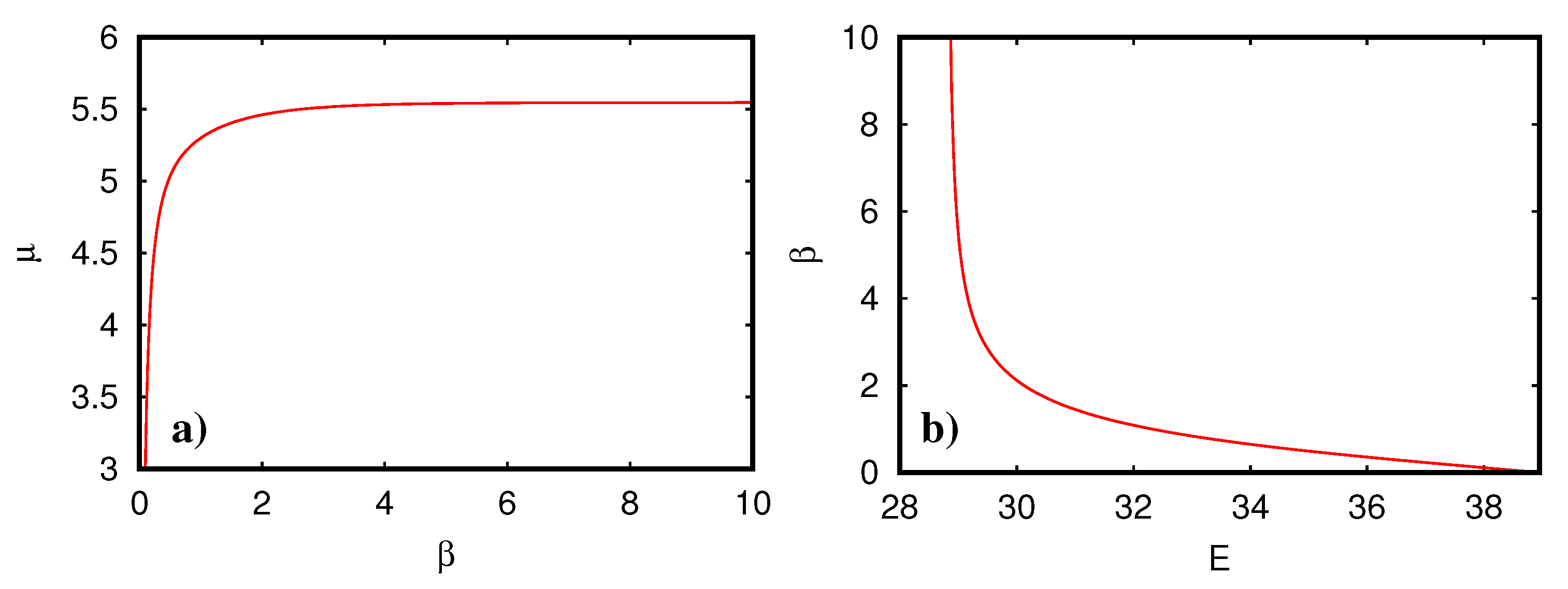
Figure 3 shows the mutual dependence between the three parameters β , μ on E when solving the conditions (12). The chemical potential as a function of β = 1 / T is rather constant except for smallest values of β where μ 1 / β with a negative prefactor. One can actually easily show from (12) that in the limit β 0 the chemical potential does not depend on ε k and is given by μ = ln [ 1 + ( M 2 L ) / L ] / β providing a singularity if L M / 2 with negative (positive) prefactor for L < M / 2 ( L > M / 2 ) and μ = 0 for L = M / 2 . The temperature ( β 1 ) vanishes for E close to the lower energy border and diverges for E close to the band center E mean .
In Figure 4, we present the nearest level spacing distribution p ( s ) for different values of the Åberg parameter. To compute p ( s ) , we have used only the “physical” levels in the lower half of the energy spectrum and the unfolding has been done with the integrated density of states (9), where q ( E ) is replaced by a fit polynomial of degree 5. For the smallest value A = 0.2 , the distribution p ( s ) is very close to the Poisson distribution with some residual level repulsion at very small spacings. This is a quite well known effect because typically the transition from Wigner–Dyson to Poisson statistics (when tuning some suitable parameter such as the Åberg parameter from strong to weak coupling) is non-uniform in energy and happens first at larger spacings (energy differences) and then at smaller spacings. The reason is simply that two levels which by chance are initially very close are easily repelled by a small residual coupling matrix element (when slightly changing a disorder realization or similar). For A = 0.5 , there is somewhat more level repulsion at small spacings, but the distribution is still rather close to the Poisson distribution with some modest deviations for s 1.2 . For the larger Åberg values A = 3.5 and A = 10 , we clearly obtain Wigner–Dyson statistics (taking into account the quite limited number of only d / 2 1 = 5719 level spacing values for the histograms). These results clearly confirm that the transition from A < 1 to A > 1 corresponds indeed to a transition from a perturbative regime to a regime of chaotic mixing with Wigner–Dyson level statistics [14].
A further confirmation that A = 1 is critical can be seen in Figure 5, which compares the dependence of the entropy S of exact eigenstates (lower half of the spectrum) on E 1 p or E ex with the theoretical thermalized entropy S th ( E ) . For the Åberg values A = 0.2 (and A = 0.5 ), the entropy S of all (most) states is significantly below its theoretical value S th . Actually, the distribution of data points is considerably concentrated at smaller entropy values which is not so clearly visible in Figure. In particular, the average of the ratio of S / S th ( E 1 p ) is 0.178 for A = 0.2 and 0.522 for A = 0.5 . For the Åberg values A = 3.5 and A = 10 , most or nearly all entropy values (for E 1 p ) are very close to the theoretical line with the average ratio S / S th ( E 1 p ) being 0.990 for A = 3.5 and 0.998 for A = 10 . For A = 3.5 , the states with lowest energies are not yet perfectly thermalized and the data points for E ex and E 1 p are still rather close. For A = 10 , all states are well thermalized (when using the energy E 1 p ) while the data points for E ex are quite outside the theoretical curve simply due to the overall increase of the width of the energy spectrum. This observation is also in agreement with the discussion of Figure 2. For smaller values A < 0.2 (not shown in Figure 5), we find that the data points are still closer to the E-axis while, for larger values A > 10 , the data points are clearly on the theoretical curve for E 1 p (but more concentrated on energy values closer to the center with larger entropy values and larger temperatures), while, for E ex , according to (10), the overall width of the exact eigenvalue spectrum increases strongly and the data points are clearly outside the theoretical curve (except for a few states close to the band center).
We note that the data points in Figure 5a,b significantly deviate from the theoretical thermalization curve since the Åberg criterion is not satisfied ( A < 1 ) . For A = 3.5 ; 10 , the deviations are significantly reduced, but they are still more pronounced in a vicinity of the ground state in agreement with the relation (1).
In Figure 6, the occupation numbers n k (averaged over several energy eigenvalues inside a given energy cell) are shown in the plane of energy E and orbital index k as color density plot for the Åberg parameter A = 3.5 . The comparison with the theoretical occupation numbers n ( ε k ) (shown in the same way) provides further confirmation that, at A = 3.5 , there is indeed already a quite strong thermalization of most eigenstates.

3.6. Thermalization of Quantum Time Evolution

The question arises how or if a time dependent state | ψ ( t ) > = exp ( i H t ) | ψ ( 0 ) > , obeying the quantum time evolution with the Hamiltonian H and an initial state | ψ ( 0 ) > being a non-interacting eigenstate | n M n 2 n 1 ) > (with all n k { 0 , 1 } and k n k = L ), evolves eventually into a thermalized state. We have computed such time dependent states using the exact eigenvalues and eigenvectors of H to evaluate the time evolution operator. As initial states, we have chosen four states (for M = 16 , L = 7 ): (i) | ϕ 1 > = | 0000100000111111 > where a particle at orbital 7 is excited from the non-interacting ground state (with all orbitals from 1 to 7 occupied) to the orbital 12, (ii) | ϕ 2 > = | 0010100000011111 > where two particles at orbitals 6 and 7 are excited from the non-interacting ground state to the orbitals 12 and 14, (iii) | ϕ 3 > = | 0000011000110111 > and (iv) | ϕ 4 > = | 1000100011001011 > . The states | ϕ 3 > and | ϕ 4 > are obtained from the exact eigenstate of H for A = 0.35 at level number m = 123 and 1354, respectively, by rounding the occupation numbers n k to 1 (or 0) if n k > 0.5 ( n k < 0.5 ) (states of top panels in Figure 2). The approximate energies (6) of these four states are E 30 ( | ϕ 1 > ), E 32 ( | ϕ 2 > and | ϕ 3 > ) and E 35 ( | ϕ 4 > ).
It is useful to express the time in multiples of the elementary quantum time step defined as:
Δ t = t H d = 1 2 π σ 2 ( A ) ,
where t H is the Heisenberg time (at the given value of A), d the dimension of the Hilbert space and σ ( A ) the width of the Gaussian density of states given in (10). The quantity Δ t is the shortest physical time scale of the system (inverse of the largest energy scale) and obviously for t Δ t the unitary evolution operator is close to the unit matrix multiplied by a uniform phase factor: exp ( i H t ) exp ( i E mean t ) 1 since the eigenvalues E m of H satisfy | E m E mean | σ ( A ) . We expect that any signification deviation of | ψ ( t ) > with respect to the initial condition | ψ ( 0 ) > happens at t Δ t (or later in case of very weak interaction). Furthermore, by analyzing the time evolution in terms of the ratio t / Δ t the results do not depend on the global energy scale of the spectral width. The longest time scale is the Heisenberg time t H 10 4 Δ t (since d = 11440 for M = 16 , L = 7 ). Later, we also discuss intermediate time scales such as the inverse decay rate obtained from the Fermi golden rule.
To show graphically the time evolution, we compute the time dependent occupation numbers n k ( t ) = < ψ ( t ) | c k c k | ψ ( t ) > and present them in a color density plot in the plane ( k , t / Δ t ) . In addition, at the time value used last, we compute the effective total one-particle energy E 1 p using the relation (11) (note that E 1 p is not conserved with respect to the time evolution except for very weak interaction) and use this value to determine from (12) the inverse temperature β , chemical potential μ and the thermalized Fermi–Dirac filling factor n ( ε k ) at each k value for the orbital index. These values of ideally thermalized occupation numbers will be shown in an additional vertical bar ( Note that this additional bar is not related to the usual color bar that provides the translation of colors to n k values). The latter is shown in Figure 6 and applies also to all subsequent figures with color density plots for n k values right behind the data for the last time values separated by a vertical white line. This presentation allows for an easy verification if the occupation numbers at the last time values are indeed thermalized or not.
In Figure 7, we show the time evolution for the initial state | ϕ 1 > and the two Åberg parameter values A = 1 and A = 3.5 using a linear time scale with integer multiples of Δ t and for t 2000 Δ t t H / 6 . At A = 1 , the occupation number n 12 (of the excited particle) shows, at the beginning, a periodic structure, with an approximate period 400 Δ t for t < 1000 Δ t , and a modest decay for t > 1000 Δ t . At the same time, the first orbitals above the Fermi sea are slightly excited. At final t = 2000 Δ t , the state is clearly not thermalized. For A = 3.5 , we see a very rapid partial decay of n 6 and n 12 together with an increase of n 7 . Furthermore, for n k with 8 k 11 , there are later and more modest excitations with a periodic time structure. Here, the final state at t = 2000 Δ t is also not thermalized, but it is closer to thermalization as for the case A = 1 .
The linear time scale used in Figure 7 is not very convenient since it cannot capture a rapid decay/increase of n k well at small times and its maximal time value is also significantly limited below the Heisenberg time. Therefore, we use in Figure 8 and Figure 9 a logarithmic time scale with 0.1 Δ t t 10 6 Δ t 10 2 t H . Note that, in these figures, the different n k values for each cell are not time averaged but represent the precise values for certain, exponentially increasing, discrete time values (see caption of Figure 8 for the precise values). Therefore, in case of periodic oscillations of n k , there will be, for larger time values, a quasi random selection of different time positions with respect to the period.
In Figure 8, the time evolution for the initial states | ϕ 1 > and | ϕ 2 > is shown for the Åberg values A = 1 , 3.5 , 10 . For | ϕ 1 > at A = 1 and A = 3.5 , the observations of Figure 7 are confirmed with the further information that the absence of thermalization in these cases is also valid for time scales larger than 2000 Δ t up to 10 6 Δ t and for A = 3.5 the initial decay of n 6 and n 12 happens at t 10 Δ t . For | ϕ 1 > at A = 10 , the decay starts at t 3 Δ t and an approximate thermalization happens at t > 40 Δ t . However, here there is still some time periodic structure and it would be necessary to do some time average to have perfect thermalization. For | ϕ 2 > at A = 1 , the decay of excited orbitals 12 and 14 starts at t 100 Δ t and saturates at t 1000 Δ t at which time also orbitals 6 and 7 are excited. After this, there are very small excitations of orbitals 8, 9, 10 and maybe 13, 15. There is also some very modest decay of the Fermi sea orbitals 2, 4 and 5 at t > 1000 Δ t . The final state at t = 10 6 Δ t is not thermalized even though some orbitals have n k values close to thermalization. For | ϕ 2 > at A = 3.5 , the decay of excited orbitals 12 and 14 starts at t 10 Δ t and, for t > 300 Δ t , there is thermalization (but requiring some time average as for | ϕ 1 > at A = 10 ). Interestingly, at intermediate times 10 Δ t < t < 100 Δ t , the high orbitals 13 and 16 are temporarily slightly excited and decay afterwards rather quickly to their thermalized values. For | ϕ 2 > at A = 10 , the decay of excited orbitals 12 and 14 starts even at t 3 Δ t and thermalization seems to set in at t > 30 Δ t .
Figure 9 is similar to Figure 8 except for the initial states | ϕ 3 > and | ϕ 4 > which have occupation numbers n k { 0 , 1 } obtained by rounding the n k values of the two eigenstates visible in the two top panels of Figure 2. Here, the initial decay of excited orbitals starts roughly at t 300 Δ t ( t ( 10 20 ) Δ t or t ( 2 3 ) Δ t ) for A = 1 ( A = 3.5 or A = 10 , respectively). There is no thermalization for both states at A = 1 (but some n k values are close to thermalized values), approximate thermalization for A = 3.5 and | ϕ 3 > and good thermalization for A = 3.5 and | ϕ 4 > as well as A = 10 (both states).
Using the time dependent values n k ( t ) , one can immediately determine the corresponding entropy S ( t ) using (11). At t = 0 , we have obviously S ( 0 ) = 0 , since, for all four initially considered states, we have perfect occupation number values of either n k = 0 or n k = 1 . Naturally, one would expect that the entropy increases with a certain rate and saturates then at some maximal value which may correspond (or be lower) to the thermalized entropy S th ( E 1 p ) (with E 1 p determined for the state | ψ ( t ) > at large times) depending if there is presence (or absence) of thermalization according to the different cases visible in Figure 8 and Figure 9. However, in the absence of thermalization, we see that there may also exist periodic oscillations with a finite amplitude at very long time scales.
In Figure 10, we show the time dependent entropy S ( t ) for the two initial states | ϕ 1 > , | ϕ 4 > and the three values A = 1 , A = 3.5 and A = 10 of the Åberg parameter. For A = 10 , there is indeed a rather rapid saturation of the entropy of both states at a maximal value that is indeed close to the thermalized entropy S th ( E 1 p ) . We note that E 1 p is not conserved at strong interactions and that its initial value E 1 p 30 ( E 1 p 35 ) at t = 0 evolves to E 1 p 33.5 ( E 1 p 37 ) at large times for | ϕ 1 > ( | ϕ 4 > ) corresponding roughly to S S th ( E 1 p ) 9.2 ( 10.8 ) visible as thin blue horizontal lines in Figure 10. For A = 3.5 (or A = 1 ), the thermalized entropy values, visible as thin green (red) lines, are lower as compared to the case A = 10 due to different final E 1 p values. For A = 3.5 and | ϕ 4 > , there is also saturation of S to its thermalized value. For A = 3.5 and | ϕ 1 > , there seems to be an approximate saturation at a quite low value S 6 but with periodic fluctuations in the range 6 ± 0.3 . For A = 1 and | ϕ 4 > , there is a quite late and approximate saturation with some fluctuations that are visible for t > 10 4 Δ t and with S 10 ± 0.2 . For A = 1 and | ϕ 1 > , there is a late periodic regime for t > 10 3 Δ with a quite large amplitude S 3 ± 1 and with S max 4 significantly below the thermalized entropy S th ( E 1 p ) 5.5 . The panels using a normal (instead of logarithmic) time scale with t 200 Δ t miss completely the long time limits for A = 1 and might incorrectly suggest that there is an early saturation at quite low values of S.
The periodic (or quasi-periodic) time dependence of n k ( t ) or S ( t ) , for the cases with lower values of A and/or an initial state with lower energy, indicates that, for such states, only a small number ( 2 , 3 , ) of exact eigenstates of H contribute mostly in the expansion of | ψ ( t ) > in terms of these eigenstates.
Figure 10 also shows that the initial increase of S ( t ) is rather comparable between the two states for identical values of A even though the long time limit might be very different. Furthermore, a closer inspection of the data indicates that typically S ( t ) is close to a quadratic behavior for t Δ t but which immediately becomes linear for t Δ t similarly as the transition probabilities between states in the context of time dependent perturbation theory. To study the approximate slope in the linear regime, we define (For practical reasons, we decide to incorporate the quantum time step Δ t in the definition of Γ c , i.e., Γ c is defined as the ratio of the initial slope S ( t ) over the global spectral bandwidth σ ( A ) 1 / Δ t ) the quantity Γ c = d S ( t ) / d ( t / Δ t ) = Δ t S ( t ) for t = ξ Δ t , where ξ 1 is a numerical constant of order one. To determine Γ c practically, we perform first the fit S ( t ) = S ¯ ( 1 exp [ γ ¯ 1 ( t / Δ t ) ] ) for 0 t / Δ t 100 and use the exponential decay rate γ ¯ 1 to perform a refined fit S ( t ) = S ( 1 exp [ γ 1 ( t / Δ t ) γ 2 ( t / Δ t ) 2 ] ) for the interval 0 t / Δ t 5 / γ ¯ 1 . From this, we determine Γ c = S γ 1 , which is rather close to S ¯ γ ¯ 1 for A 2 but not for larger values of A where the decay time is reduced and not sufficiently large in comparison to the initial quadratic regime. Therefore, the quadratic term in the exponential is indeed necessary to obtain a reasonable fit quality. This procedure corresponds to an effective average of the value of ξ between 1 and roughly 1 / γ 1 , which is indeed useful to smear out some oscillations in the initial increase of S ( t ) for smaller values A 1 .
We note that, for many-body quantum systems, the exponential growth of entropy with time had been also discussed and numerically illustrated in [40] (see also related publications in References 25 and 26 there). Recently, such an exponential growth of entropy has been discussed in [62,70].
Figure 11 shows the dependence of these values of Γ c on the parameter A for our four initial states. At first sight, one observes a behavior Γ c A 2 for A 2 and a saturation for larger values of A. However, a more careful analysis shows that there are modest but clearly visible deviations with respect to the quadratic behavior in A (power law fits Γ c A p for A 2 provide exponents close to p 1.75 1.85 ) and it turns out that these deviations correspond to a logarithmic correction: Γ c = f ( A ) = ( C 1 C 2 ln [ g ( A ) ] ) g ( A ) with g ( A ) = A 2 (for fits with A 1 ) or with g ( A ) = A 2 / ( 1 + C 3 A 2 ) (for fits with all A values).
To understand this behavior, we write for sufficiently small times n k ( t ) 1 δ n k ( t ) (if n k ( 0 ) = 1 ) or n k ( t ) δ n k ( t ) (if n k ( 0 ) = 0 ), where δ n k ( t ) is the small modification of n k ( t ) . Time dependent perturbation theory suggests that δ n k ( t ) ( t / Δ t ) 2 for t Δ t and δ n k ( t ) a k A 2 t / Δ t for t Δ t such that still δ n k ( t ) 1 with coefficients a k dependent on k (and also on M, L) and satisfying a linear relation to ensure the conservation of particle number. Using (11) and neglecting corrections of order δ n k 2 , we obtain: S k δ n k ln δ n k δ n k and Γ c = Δ t S ( t ) Δ t k δ n k ( t ) ln δ n k ( t ) with t = ξ Δ t . Since δ n k ( t ) a k A 2 / Δ t , we find indeed the behavior:
Γ c = [ C 1 C 2 ln ( A 2 ) ] A 2 , C 1 = k a k ln ( a k ξ ) , C 2 = k a k ,
where indicates an average over some modest values of ξ 1 . The precise values of a k may depend rather strongly on the orbital index k and the initial state (see also Figure 8 and Figure 9), but the coefficients C 1 , C 2 depend only slightly on the initial state (see Table 2). Furthermore, by replacing A 2 g ( A ) = A 2 / ( 1 + C 3 A 2 ) to allow for a saturation at large A and with a further fit parameter C 3 , it is possible to describe the numerical data by the more general fit Γ c = f ( a ) for the full range of A values.

3.7. Survival Probability and Fermi’s Golden Rule

The knowledge of the time dependent states | ψ ( t ) > allows us also to compute the decay function p dec ( t ) = | < ψ ( 0 ) | ψ ( t ) > | 2 which represents the survival probability of the initial non-interacting eigenstate due to the influence of interactions. Again, for the very short time window t Δ t , we expect a quadratic decay: 1 p dec ( t ) ( H E mean ) 2 t 2 const . ( t / Δ t ) 2 with being the quantum expectation value with respect to | ψ ( 0 ) > and a numerical constant 1 since 1 / Δ t represents roughly the spectral width of H. For t Δ t , but such that 1 p dec ( t ) 1 , we have, according to Fermi’s golden rule: 1 p dec ( t ) = Γ F ( t / Δ t ) , where Γ F is the decay rate (Again, for practical reasons and similarly to Γ c , we incorporate in the definition of Γ F the time scale Δ t , i.e., Γ F = Δ t × usual decay rate found in the literature and meaning that Γ F is defined as the ratio of the usual decay rate over the global spectral bandwidth) of the state.
To determine Γ F numerically, we apply the fit: p dec ( t ) = C exp ( Γ F t / Δ t ) in two steps. First, we use the interval 1 t / Δ t 50 and, if 5 / Γ F < 50 , corresponding to a rapid decay (which happens for larger values of A), we repeat the fit for the reduced interval 1 t / Δ t 5 / Γ F . The choice of the Amplitude C 1 and the condition t Δ t for the fit range allow for taking into account the effects due to the small initial window of quadratic decay. In Figure 12, we show two examples for the initial state | ϕ 1 > and the Åberg values A = 3.5 and A = 10 . In both cases, the shown maximal time value t max = 50 Δ t (if A = 3.5 ) or t max 13.5 (if A = 10 ) defines the maximal time value for the fit range. For A = 10 , the fit nicely captures the decay for 1 t / Δ t 6 , while, for A = 3.5 , there are also some oscillations in the decay function for which the fit procedure is equivalent to some suitable average in the range 1 t / Δ t 30 . For very small values of A, the fit procedure also works correctly since it captures only the initial decay that is important if p dec ( t ) does not decay completely at large times and which typically happens in the perturbative regime A 1 .
Figure 13 shows the dependence of Γ F on A for the usual four initial states together with the fit Γ F = f ( A ) = C 4 A 2 / ( 1 + C 5 A 2 ) for the data with initial state | ϕ 1 > . The values of the parameters C 4 , C 5 for this and the other initial states are given in Table 2. Here, the initial quadratic dependence Γ F A 2 is highly accurate (with no logarithmic correction). Similarly to Γ c , there is only a slight dependence of the values of Γ F and the fit values on the choice of initial state.
Theoretically, we expect according to Fermi’s Golden rule that: Γ F ( Δ t ) 2 π V Fock 2 ρ c ( E ) , where V Fock 2 = T r Fock ( V 2 ) / ( K d ) = σ 0 2 α A 2 / K according to the discussion below (10) and ρ c ( E ) is the effective two-body density of states for states directly coupled by the interaction such that ρ c ( E mean ) = 1 / Δ c (see discussion below (7)). We note that V Fock is the typical interaction matrix element in Fock space which is slightly larger than V mean (see the theoretical discussion above for the computation of the coefficient α used in (10) and Appendix A of [46]). The factor Δ t is due to our particular definition (Again, for practical reasons and similarly to Γ c , we incorporate in the definition of Γ F the time scale Δ t , i.e., Γ F = Δ t × usual decay rate found in the literature and meaning that Γ F is defined as the ratio of the usual decay rate over the global spectral bandwidth) of decay rates. The expression of Γ F is actually also valid for larger values of A provided we use the density of states ρ c ( E ) in the presence of interactions that provides an additional factor 1 / 1 + α A 2 according to (10). Therefore, at the band center, we have: 2 π Δ t ρ c = K / [ σ 0 ( L ) σ 0 ( L = 2 ) ( 1 + α A 2 ) ] , which gives, together with (8):
Γ F = σ 0 ( L ) σ 0 ( L = 2 ) α A 2 1 + α A 2 = L ( M L ) 2 ( M 2 ) α A 2 1 + α A 2 .
For M = 16 and L = 7 , the square root factor is 1.5 and we have to compare 1.5 α 0.0132 with the values of C 4 in Table 1, which are somewhat smaller, probably due to a reduction factor for the energy dependent density of states since the energies of the initial states have a certain distance to the band center. Furthermore, according to (15), we have to compare C 5 with α 0.00877 which is not perfect but gives the correct order of magnitude. For both parameters, the numerical matching is quite satisfactory taking into account the very simple argument using the same typical value of the interaction matrix elements for all cases of initial states.
Finally, we mention that, for the three Åberg parameter values A = 1 , A = 3.5 , A = 10 used in Figure 8 and Figure 9, we have typical decay times in units of Δ t being 1 / Γ F 300 , 30, 3, respectively (with some modest fluctuations depending on initial states). These values match quite well the observed time values at which the initially occupied orbitals start to decay (see the above discussion of Figure 8 and Figure 9).

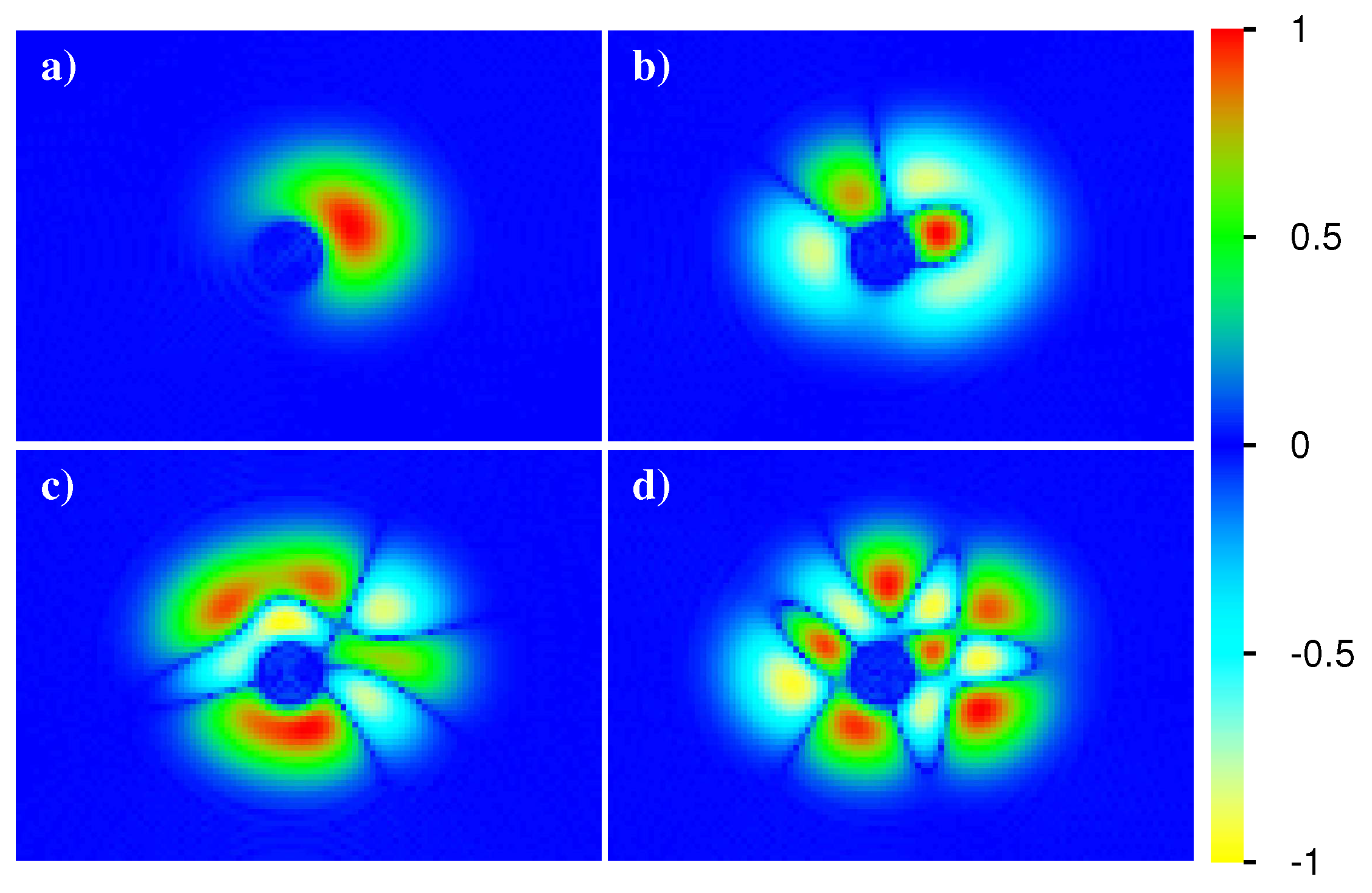
3.8. Time Evolution of Density Matrix and Spatial Density

We now turn to the effects of the many-body time evolution in position space (see for example Figure 1). For this, we compute the spatial density
ρ ( x , y , t ) = < ψ ( t ) | Ψ ( x , y ) Ψ ( x , y ) | ψ ( t ) > , Ψ ( ) ( x , y ) = k φ k ( * ) ( x , y ) c k ( ) ,
where φ k ( x , y ) is the one-particle eigenstate of orbital k, with some examples shown in Figure 1. Here, Ψ ( ) ( x , y ) denotes the usual fermion field operators (in the case of continuous x, y variables) or standard fermion operators for discrete position basis states (when using a discrete grid for x and y positions as we did for the numerical solution of the non-interacting Sinai oscillator model in Section 2). The sum over orbital index k in (16) requires in principle a sum over a full complete basis set of orbitals with infinite number (case of continuous x, y values) or a very large number (case of discrete x-y grid) significantly larger than the very modest number of orbitals M we used for the numerical solution of the many-body Sinai oscillator.
However, we can simply state that, in our model, by construction, all orbitals with k > M are never occupied such that, in the expectation value for ρ ( x , y , t ) , only the values k M are necessary. Taking this into account together with the fact that the one-particle eigenstates are real valued, we obtain the more explicit expression:
ρ ( x , y ; t ) = k , l = 1 M φ k ( x , y ) φ l ( x , y ) n k l ( t ) , n k l ( t ) = < ψ ( t ) | c k c l | ψ ( t ) > ,
where n k l ( t ) is the density matrix in orbital representation generalizing the occupation numbers n k ( t ) which are its diagonal elements. Due to the complex phases of | ψ ( t ) > (when expanded in the usual basis of non-interacting many-body states), the density matrix is complex valued but hermitian: n k l * ( t ) = n l k ( t ) . Therefore, its anti-symmetric imaginary part does not contribute in ρ ( x , y ; t ) . We have numerically evaluated (17) and we present in Figure 14 color plots of the density matrix and the spatial density ρ ( x , y ; t ) for A = 3.5 , the initial state | ψ ( 0 ) > = | ϕ 2 > and four time values t / Δ t = 0.1 , 30 , 100 , 1000 . Since the density ρ ( x , y ; t ) does not provide a lot of spatial structure, we also show in Figure 14 the density difference with respect to the initial condition Δ ρ ( x , y ; t ) = ρ ( x , y ; t ) ρ ( x , y ; 0 ) which reveals more of its structure (figures and videos for the time evolution of this and other cases are available for download at the web page [71]).
At the time t / Δ t = 0.1 , density matrix and spatial density are essentially identical to the initial condition at t = 0 . For Δ ρ , we see a non-trivial structure since there is a small difference with the initial condition and the color plot simply amplifies small maximal amplitudes to maximal color values (red/yellow for strongest positive/negative values even if the latter are small in an absolute scale). The density matrix is diagonal and its diagonal values are either 1 (for initially occupied orbitals) or 0 (for initially empty orbitals) and the spatial density simply gives the sum of densities due to the occupied eigenstates.
At t / Δ t = 30 , we see a non-trivial structure in the density matrix with a lot of non-vanishing values in certain off-diagonal elements. Furthermore, the orbitals 13 and 16 are also slightly excited (see also discussion of Figure 8) and there is a significant change of the spatial density.
Later, at t / Δ t = 100 , the number/values of off-diagonal elements in the density matrix is somewhat reduced, but they are still visible. Especially between orbitals 12 and 13 as well as 14 and 15, there is a rather strong coupling. Orbital 13 is now more strongly excited than the initially excited orbital 12. In addition, orbitals 14 and 15 are quite strong. The spatial density has become smoother and the structure of Δ ρ is roughly close to the case at t / Δ t = 30 but with some significant differences.
Finally, at t / Δ t = 1000 , the density matrix seems be diagonal with values close to the thermalized values. There is a further increase of the density smoothness and Δ ρ has a similar but different structure as for t / Δ t = 100 or t / Δ t = 30 .
Apparently, at intermediate times 20 t / Δ t 100 , there are some quantum correlations between certain orbitals, visible as off-diagonal elements in the density matrix which disappear for later times. This kind of decoherence is similar to the exponential decay observed in [46] for the off-diagonal element of the 2 × 2 density matrix for a qubit coupled to a chaotic quantum dot or the SYK black hole. However, to study this kind of decoherence more carefully in the context here, it would be necessary to use as initial state a non-trivial linear combination of two non-interacting eigenstates and not to rely on the creation of modest off-diagonal elements for intermediate time scales as we see here.
The spatial density is globally rather smooth and typically quite well given by the “classical” relation ρ ( x , y ; t ) k φ k 2 ( x , y ) n k ( t ) in terms of the time dependent occupation numbers. Only for intermediate time scales with more visible quantum coherence (more off-diagonal elements n k l ( t ) 0 ), this relation is less accurate. However, at A = 3.5 , the density still exhibits small but regular fluctuations in its detail structure as can be seen in the structure of Δ ρ for later time scales. A closer inspection of the data (for time values not shown in Figure 14) also shows that, even at long time scales, there are significant fluctuations of ρ when t is slightly changed by a few multiples of Δ t .
In Figure 14, we also show for comparison the theoretical thermalized quantities where, in (17), the density matrix is replaced by a diagonal matrix with entries being the thermalized occupations numbers n k k = n ( ε k ) at energy E = 32.9 , which is the typical total one-particle average energy of | ψ ( t ) > for the long time limit t / Δ t 1000 showing that, at t / Δ t = 1000 , the state is very close to thermalization but still with small significant differences (see also discussion of Figure 7 for this case).
We may also generalize the spatial density (16) to a spatial density correlator which we define as:
ρ corr ( x , y ; x 0 , y 0 ; t ) = < ψ ( t ) | Ψ ( x , y ) Ψ ( x 0 , y 0 ) | ψ ( t ) > = k , l = 1 M φ k ( x , y ) φ l ( x 0 , y 0 ) n k l ( t )
depending on initial ( x 0 , y 0 ) and final position ( x , y ) . As an illustration, we choose the fixed value ( x 0 , y 0 ) = ( 1.22 , 0.15 ) which is very close to the maximal position (center of the red area) of the one-particle ground state φ 1 ( x , y ) visible in panel (a) of Figure 1. The spatial density correlator is potentially complex with a non-vanishing imaginary part in case of non-vanishing off-diagonal matrix elements of n k l ( t ) 0 for k l . In Figure 15, we present density plots of absolute value, real and imaginary part of ρ corr ( x , y ; x 0 , y 0 ; t ) in ( x , y ) plane and with the given value ( x 0 , y 0 ) = ( 1.22 , 0.15 ) for the same parameters of Figure 14 (concerning initial state, Åberg parameter, time values and also thermalized case). However, for the thermalized case, the density matrix is diagonal by construction and the imaginary part of ρ corr , th ( x , y ; x 0 , y 0 ) vanishes (giving a blue panel due to zero values).
There are significant time dependent fluctuations of ρ corr ( x , y ; x 0 , y 0 ; t ) for all time scales with real part and absolute value being dominated by rather strong maximal values for positions close to the initial position. However, the imaginary part (which vanishes at t = 0 and is typically smaller than the values in maximum domain of a real part) shows a more interesting structure since the color plot amplifies small amplitudes (in absolute scale). Apart from this, the absolute and real part values for positions outside the maximum domain (far away from the initial position) seem to decay for long timescales, which is also confirmed by the thermalized case. Even though the case for t / Δ t = 1000 seems to be rather close to the thermalized case (for absolute value and real part), there are still differences that are more significant here as in Figure 14.
Globally, the obtained results show that the dynamical thermalization takes place well, leading to the usual Fermi–Dirac thermal distribution when the Åberg criterion is satisfied and interactions are sufficiently strong to drive the system into the thermal state.

4. Estimates for Cold Atom Experiments

We discuss here typical parameters for cold atoms in a trap following [72]. Thus, for sodium atoms, we have ω ω x , y , z 2 π 10 H z with a 0 = / ( m ω ) = 6.5 μ m and oscillator level spacing E u = ω 0.5 n K (nanoKelvin). The typical scattering length is a s 3 n m being small compared to a 0 . The atomic density is ρ 0 = 1 / ( a 0 ) 3 4 × 10 9 c m 3 . Since a s a 0 , the two-body interaction is of δ -function type with v ( r 1 r 2 ) = ( 4 π 2 a s / m ) δ ( r 1 r 2 ) [66,72]. In our numerical simulations, δ ( r ) is replaced by a function H ( r c | r | ) / ( C 2 d r c d ) with a small r c , volume C of the unit sphere in d dimensions and with the Heaviside function H ( x ) = 1 (or 0) for x 0 and H = 0 for x < 0 . Hence, our parameter U introduced in Section 3 corresponds to U = ( C 2 d r c d ) ( 4 π 2 a s / m ) .
Below, we present the estimates for the dynamical thermalization border for excitations of fermionic atoms in a vicinity of their Fermi energy in a 3D Sinai oscillator following the lines of Equation (1). In such a case, the two-body interaction energy scale between atoms is U s = 4 π 2 ρ 0 a s / m = 4 π ( a s / a 0 ) ω [66,72] so that U s / ω 6 × 10 3 . Compared to sodium, the mass of Li atoms is approximately three times smaller so that, for the same ω , we have a 0 10 μ m and U s / ω 4 × 10 3 . We think that the scattering length can be significantly increased via the Feshbach resonance, allowing for reaching effective interaction values U s / ω 1 being similar to the value A 3 used in our numerical studies with the onset of dynamical thermalization.
Usually, a 3D trap with fermionic atoms can capture about N a 10 5 atoms with ω ω x ω y ω z 2 π 10 H z . Following the result (1), it is interesting to determine the DTC border dependence on N a 1 for a Sinai oscillator with r d 1 μ m a 0 / 5 . We assume that, similar to a 2D case, the scattering on an elastic ball in the trap center leads to quantum chaos and chaotic eigenstates with N a components (e.g., in the basis of oscillator eigenfunctions). The Fermi energy of the trap is then E F = ( N a ω x ω y ω z ) 1 / 3 ω N a 1 / 3 [52,53]. Assuming that all these components have random amplitudes of a typical size 1 / , we then obtain an estimate for a typical matrix element of two-body interaction between one-particle eigenstates
U 2 α s ω / 3 / 2 , α s = 4 π ( a s / a 0 ) , a 0 = / m ω .
The derivation of this estimate is very similar to the case of two interacting particles in a disordered potential with localized eigenstates [73]. At the same time, in the vicinity of the Fermi energy E F , we have the one-particle level spacing Δ 1 = d E F / d N a ω / ( 3 N a 2 / 3 ) . Hence, the effective conductance appears in in (1) is g = Δ 1 / U 2 3 / 2 / ( 3 α s N a 2 / 3 ) . Thus, from (1), we obtain the dynamical thermalization border for excitation energy δ E in a 3D Sinai oscillator trap with N a fermionic atoms:
δ E > δ E c h Δ 1 g 2 / 3 2 Δ 1 / ( α s 2 / 3 N a 4 / 9 ) N a 5 / 9 Δ 1 / α s 2 / 3 ω / ( α s 2 / 3 N a 1 / 9 ) E F / ( α s 2 / 3 N a 4 / 9 ) .
It is assumed that δ E E F . Here, the last three relations are written in an assumption that N a . Thus, at large N a values and not too small α s , the critical energy border δ E c h for dynamical thermalization is rather small compared to E F . However, still δ E c h Δ 1 . Here, we used the maximal value for the number of components N a . It is possible that, in reality, can be significantly smaller than N a . However, the determination of the dependence ( N a ) requires separate studies taking into account the properties of chaotic eigenstates and their spreading over the energy surface. This spreading can have rather nontrivial properties (see, e.g., [23]). This is confirmed by the results presented in Appendix A for the 2D case of Sinai oscillator showing the numerically obtained dependence of two-body matrix elements on energy for transitions in a vicinity of Fermi energy E F (see Figure A1 there).

5. Conclusions

In this work, we demonstrated the existence of interaction induced dynamical thermalization of fermionic atoms in a Sinai oscillator trap if the interaction strength between atoms exceeds a critical border determined by the Åberg criterion [38,39,41]. This thermalization takes place in a completely isolated system in the absence of any contact with an external thermostat. In the context of the Loschmidt–Boltzmann dispute [1,2], we should say that formally this thermalization is reversible in time since the Schrodinger equation of the system has symmetry t t . The classically chaotic dynamics of atoms in the Sinai oscillator trap breaks in practice this reversibility due to exponential growth of errors induced by chaos. In the regime of quantum chaos, there is no exponential growth of errors due to the fact that the Ehrenfest time scale of chaos is logarithmically short [17,19,26,28]. An example for the stability of time reversibility is given in [27,28]. In fact, the experimental reversal of atom waves in the regime of quantum chaos has been even observed with cold atoms in [74]. In view of this and the fact that the spectrum of atoms in the Sinai oscillator trap is discrete, we can say that dynamical thermalization will have obligatory revivals in time returning from the thermalized state (e.g., bottom panels in Figure 8) to the initial state (top panels in Figure 8). This is the direct consequence of the Poincare recurrence theorem [75]. However, the time for such a recurrence grows exponentially with the number of components contributing to the initial state (which is also exponentially large in the regime of dynamical thermalization) and thus, during such a long time scale, external perturbations (coming from outside of our isolated system, e.g., not perfect isolation) will break in practice this time reversibility.
We hope that our results will initiate experimental studies of dynamical thermalization with cold fermionic atoms in systems such as the Sinai oscillator trap.

Author Contributions

All authors equally contributed to all stages of this work.

Funding

This work was supported in part by the Programme Investissements d’Avenir ANR-11-IDEX-0002-02, reference ANR-10-LABX-0037-NEXT (project THETRACOM). This work was granted access to the HPC GPU resources of CALMIP (Toulouse) under the allocation 2018-P0110.

Acknowledgments

We are thankful to Shmuel Fishman for deep discussions of quantum chaos problems and related scientific topics during many years.

Conflicts of Interest

The authors declare no conflict of interest.

Appendix A. Two-Body Matrix Elements near the Fermi Energy

In this Appendix, we present numerical results for the dependence of the quantity V mean ( ε ) = V i j , k l 2 as a function of ε where the average is done only for orbitals with energies ε n close to ε (for n { i , j , k , l } ), i.e.: | ε n ε | Δ ε with Δ ε = 2 . We note that this is different from the quantity V mean used in Section 3 where the average was done over all orbitals (up to a maximal number being M). The reason for the special average with orbital energies close to ε (which will be identified with the Fermi energy E F ) is that these transitions are dominant in the presence of the Pauli blockade near the Fermi level.
We remind readers that, according to the discussion of Section 2 and Section 3, the matrix elements V i j , k l were computed for an interaction potential of amplitude U for | r 1 r 2 | < r c (with the radius r c = 0.2 r d = 0.2 ) and being zero for | r 1 r 2 | r c . Furthermore, they have been anti-symmetrized and a diagonal shift V i j , i j V i j , i j ( 1 / M 2 ) k < l V k l , k l was applied to ensure that the interaction matrix has a vanishing trace.
Due to this shift and the precise average procedure, there is a slight (purely theoretical) dependence on the maximal orbital number M for this average (there is a cut-off effect for ε close to the maximal orbital energy ε M ). Due to this, we considered two values of M = 30 and M = 60 .
The numerically obtained dependence is shown in Figure A1 and is well described by the fit V mean / U = a / ε b with a = 1.56 × 10 4 and b = 0.78 . The small value of a is due to antisymmetry of two-particle fermionic states and, due to a small value of r c = 0.2 r d , which leads to a decrease of the effective interaction strength being proportional to r c 2 .
Figure A1. Dependence of the average two-body matrix element V mean rescaled by the amplitude of interaction strength U on one-particle energy ε for two-body interaction transitions in a vicinity of Fermi energy E F = ε ; green symbols are for number of one-particle orbitals M = 30 , red symbols are for M = 60 ; the blue line shows the fit V mean / U = a / ε b with a = 0.000156 ± 2 × 10 6 ; b = 0.781 ± 0.005 .
Condensedmatter 04 00076 g0a1
We note that the Fermi energy is determined by the number of fermionic atoms N a inside the 2D Sinai oscillators with ε = E F ω N a 1 / 2 assuming ω = ω x ω y . Therefore, we have ε M 1 / 2 N a 1 / 2 , Δ 1 ω / N a 1 / 2 and V mean α s ω / 3 / 2 α s ω / N a b / 2 (see (19)). Hence, the obtained exponent b 0.78 corresponds to the number of one-particle components N a b / 3 N a 0.25 n x 0.5 . At the moment, we do not have a clear explanation for this numerical dependence. This dependence corresponds to g = Δ 1 / V mean 3 / 2 / ( α s N a 1 / 2 ) 1 / ( α s N a 1 / 8 ) . For such a dependence, we obtain that the DTC border in 2D takes place for an excitation energy δ E > δ E c h g 2 / 3 Δ 1 ω / ( α s 2 / 3 N a 7 / 12 ) . Thus, the thermalization can take place at rather low energy excitations above the Fermi energy with Δ 1 < δ E E F .

References

  1. Loschmidt, J. Über den Zustand des Wärmegleichgewichts eines Systems von Körpern mit Rücksicht auf die Schwerkraft; II-73; Sitzungsberichte der Akademie der Wissenschaften: Wien, Austria, 1876; pp. 128–142. [Google Scholar]
  2. Boltzmann, L. Über die Beziehung eines Allgemeine Mechanischen Satzes zum Zweiten Haupsatze der Wärmetheorie; II-75; Sitzungsberichte der Akademie der Wissenschaften: Wien, Austria, 1877; pp. 67–73. [Google Scholar]
  3. Mayer, J.E.; Goeppert-Mayer, M. Statistical Mechanics; Wiley: New York, NY, USA, 1977. [Google Scholar]
  4. Gousev, A.; Jalabert, R.A.; Pastawski, H.M.; Wisniacki, D.A. Loschmidt echo. Scholarpedia 2012, 7, 11687. [Google Scholar]
  5. Arnold, V.; Avez, A. Ergodic Problems in Classical Mechanics; Benjamin: New York, NY, USA, 1968. [Google Scholar]
  6. Cornfeld, I.P.; Fomin, S.V.; Sinai, Y.G. Ergodic Theory; Springer: New York, NY, USA, 1982. [Google Scholar]
  7. Chirikov, B.V. A universal instability of many-dimensional oscillator systems. Phys. Rep. 1979, 52, 263. [Google Scholar] [CrossRef]
  8. Lichtenberg, A.; Lieberman, M. Regular and Chaotic Dynamics; Springer: New York, NY, USA, 1992. [Google Scholar]
  9. Sinai, Y.G. Dynamical systems with elastic reflections. Ergodic properties of dispersing billiards. Uspekhi Mat. Nauk 1970, 25, 141. [Google Scholar]
  10. Gutzwiller, M.C. Chaos in Classical and Quantum Mechanics; Springer: New York, NY, USA, 1990. [Google Scholar]
  11. Haake, F. Quantum Signatures of Chaos; Springer: Berlin, Germany, 2010. [Google Scholar]
  12. Stockmann, H.-J. Microwave billiards and quantum chaos. Scholarpedia 2010, 5, 10243. [Google Scholar] [CrossRef]
  13. Bohigas, O.; Giannoni, M.J.; Schmit, C. Characterization of chaotic quantum spectra and universality of level fluctuation. Phys. Rev. Lett. 1984, 52, 1. [Google Scholar] [CrossRef]
  14. Wigner, E. Random matrices in physics. SIAM Rev. 1967, 9, 1. [Google Scholar] [CrossRef]
  15. Mehta, M.L. Random Matrices; Elsvier Academic Press: Amsterdam, The Netherlands, 2004. [Google Scholar]
  16. Ullmo, D. Bohigas-Giannoni-Schmit conjecture. Scholarpedia 2016, 11, 31721. [Google Scholar] [CrossRef]
  17. Chirikov, B.V.; Izrailev, F.M.; Shepelyansky, D.L. Dynamical stochasticity in classical and quantum mechanics. Math. Phys. Rev. 1981, 2, 209–267. [Google Scholar]
  18. Fishman, S.; Grempel, D.R.; Prange, R.E. Chaos, quantum recurrences, and Anderson localization. Phys. Rev. Lett. 1982, 49, 509. [Google Scholar] [CrossRef]
  19. Chirikov, B.V.; Izrailev, F.M.; Shepelyansky, D.L. Quantum chaos: Localization vs. ergodicity. Phys. D 1988, 33, 77. [Google Scholar] [CrossRef]
  20. Fishman, S. Anderson localization and quantum chaos maps. Scholarpedia 2010, 5, 9816. [Google Scholar] [CrossRef]
  21. Anderson, P.W. Absence of diffusion in certain random lattices. Phys. Rev. 1958, 109, 1492. [Google Scholar] [CrossRef]
  22. Frahm, K.M.; Shepelyansky, D.L. Quantum localization in rough billiards. Phys. Rev. Lett. 1997, 78, 1440. [Google Scholar] [CrossRef]
  23. Frahm, K.M.; Shepelyansky, D.L. Emergence of quantum ergodicity in rough billiards. Phys. Rev. Lett. 1997, 79, 1833. [Google Scholar] [CrossRef]
  24. Bohr, N. Über die Serienspektra der Element. Zeitschrift für Physik 1920, 2, 423. [Google Scholar] [CrossRef]
  25. Ehrenfest, P. Bemerkung über die angenäherte Gültigkeit der klassischen Mechanik innerhalb der Quantenmechanik. Zeitschrift für Physik 1927, 45, 455. [Google Scholar] [CrossRef]
  26. Shepelyanskii, D.L. Dynamical stochasticity in nonlinear quantum systems. Theor. Math. Phys. 1981, 49, 925. [Google Scholar] [CrossRef]
  27. Shepelyansky, D.L. Some statistical properties of simple classically stochastic quantum systems. Phys. D 1983, 8, 208. [Google Scholar] [CrossRef]
  28. Chirikov, B.; Shepelyansky, D. Chirikov standard map. Scholarpedia 2008, 3, 3550. [Google Scholar] [CrossRef]
  29. Bohr, A.; Mottelson, B.R. Nuclear Structure; Benjamin: New York, NY, USA, 1969; Volume 1, p. 284. [Google Scholar]
  30. Guhr, T.; Muller-Groeling, A.; Weidenmuller, H.A. Random-matrix theories in quantum physics: Common concepts. Phys. Rep. 1998, 299, 189. [Google Scholar] [CrossRef]
  31. French, J.B.; Wong, S.S.M. Validity of random matrix theories for many-particle systems. Phys. Lett. B 1970, 33, 449. [Google Scholar] [CrossRef]
  32. Bohigas, O.; Flores, J. Two-body random Hamiltonian and level density. Phys. Lett. B 1971, 34, 261. [Google Scholar] [CrossRef]
  33. French, J.B.; Wong, S.S.M. Some random-matrix level and spacing distributions for fixed-particle-rank interactions. Phys. Lett. B 1971, 35, 5. [Google Scholar] [CrossRef]
  34. Bohigas, O.; Flores, J. Spacing and individual eigenvalue distributions of two-body random Hamiltonians. Phys. Lett. B 1971, 35, 383. [Google Scholar] [CrossRef]
  35. Thouless, D.J. Maximum Metallic Resistance in Thin Wires. Phys. Rev. Lett. 1977, 39, 1167. [Google Scholar] [CrossRef]
  36. Imry, Y. Introduction to Mesoscopic Physics; Oxford University Press: Oxford, UK, 2002. [Google Scholar]
  37. Akkermans, E.; Montambaux, G. Mesoscopic Physics of Electrons and Photons; Cambridge University Press: Cambridge, UK, 2007. [Google Scholar]
  38. Åberg, S. Onset of chaos in rapidly rotating nuclei. Phys. Rev. Lett. 1990, 64, 3119. [Google Scholar] [CrossRef] [PubMed]
  39. Åberg, S. Quantum chaos and rotational damping. Prog. Part. Nucl. Phys. 1992, 28, 11. [Google Scholar] [CrossRef]
  40. Shepelyansky, D.L. Quantum chaos and quantum computers. Phys. Scr. 2001, T90, 112. [Google Scholar] [CrossRef]
  41. Jacquod, P.; Shepelyansky, D.L. Emergence of quantum chaos in finite interacting Fermi systems. Phys. Rev. Lett. 1997, 79, 1837. [Google Scholar] [CrossRef]
  42. Shepelyansky, D.L.; Sushkov, O.P. Few interacting particles in a random potential. Europhys. Lett. 1997, 37, 121. [Google Scholar] [CrossRef]
  43. Gornyi, I.V.; Mirlin, A.D.; Polyakov, D.G. Many-body delocalization transition and relaxation in a quantum dot. Phys. Rev. B 2016, 93, 125419. [Google Scholar] [CrossRef] [Green Version]
  44. Gornyi, I.V.; Mirlin, A.D.; Polyakov, D.G.; Burin, A.L. Spectral diffusion and scaling of many-body delocalization transitions. Ann. Phys. 2017, 529, 1600360. [Google Scholar] [CrossRef]
  45. Kolovsky, A.R.; Shepelyansky, D.L. Dynamical thermalization in isolated quantum dots and black holes. EPL 2019, 117, 10003. [Google Scholar] [CrossRef]
  46. Frahm, K.M.; Shepelyansky, D.L. Dynamical decoherence of a qubit coupled to a quantum dot or the SYK black hole. Eur. Phys. J. B 2018, 91, 257. [Google Scholar] [CrossRef]
  47. Landau, L.D.; Lifshitz, E.M. Statistical Mechanics; Wiley: New York, NY, USA, 1976. [Google Scholar]
  48. Ermann, L.; Vergini, E.; Shepelyansky, D.L. Dynamics and thermalization a Bose–Einstein condensate in a Sinai oscillator trap. Phys. Rev. A 2016, 94, 013618. [Google Scholar] [CrossRef]
  49. Davis, K.B.; Mewes, M.-O.; Andrews, M.R.; van Druten, N.J.; Durfee, D.S.; Kurn, D.M.; Ketterle, W. Bose–Einstein Condensation in a Gas of Sodium Atoms. Phys. Rev. Lett. 2015, 75, 3969. [Google Scholar] [CrossRef] [PubMed]
  50. Anglin, J.A.; Ketterle, W. Bose Einstein condensation of atomic gases. Nature 2002, 416, 211. [Google Scholar] [CrossRef] [PubMed]
  51. Ketterle, W. Nobel lecture: When atoms behave as waves: Bose–Einstein condensation and the atom laser. Rev. Mod. Phys. 2002, 74, 1131. [Google Scholar] [CrossRef]
  52. Valtolina, G.; Scazza, F.; Amico, A.; Burchianti, A.; Recati, A.; Enss, T.; Inguscio, M.; Zaccanti, M.; Roati, G. Exploring the ferromagnetic behaviour of a repulsive Fermi gas through spin dynamics. Nat. Phys. 2017, 13, 704. [Google Scholar] [CrossRef]
  53. Burchianti, A.; Scazza, F.; Amico, A.; Valtolina, G.; Seman, J.A.; Fort, C.; Zaccanti, M.; Inguscio, M.; Roati, G. Connecting dissipation and phase slips in a Josephson junction between fermionic superfluids. Phys. Rev. Lett. 2018, 120, 025302. [Google Scholar] [CrossRef] [PubMed]
  54. Sachdev, S.; Ye, J. Gapless spin-fluid ground state in a random quantum Heisenberg magnet. Phys. Rev. Lett. 1993, 70, 3339. [Google Scholar] [CrossRef] [PubMed]
  55. Kitaev, A. A Simple Model of Quantum Holography. Video Talks at KITP Santa Barbara, 7 April and 27 May 2015.
  56. Sachdev, S. Bekenstein-Hawking entropy and strange metals. Phys. Rev. X 2015, 5, 041025. [Google Scholar] [CrossRef]
  57. Polchinski, J.; Rosenhaus, V. The spectrum in the Sachdev-Ye-Kitaev model. J. High Energy Phys. 2016, 4, 1. [Google Scholar] [CrossRef]
  58. Maldacena, J.; Stanford, D. Remarks on the Sachdev-Ye-Kitaev model. Phys. Rev. D 2016, 94, 106002. [Google Scholar] [CrossRef] [Green Version]
  59. Garcia-Garcia, A.M.; Verbaarschot, J.J.M. Spectral and thermodynamic properties of the Sachdev-Ye-Kitaev model. Phys. Rev. D 2016, 94, 126010. [Google Scholar] [CrossRef] [Green Version]
  60. Nandkishore, R.; Huse, D.A. Many-body localization and thermalization in quantum statistical mechanics. Annu. Rev. Condens. Matter Phys. 2015, 6, 15. [Google Scholar] [CrossRef]
  61. Alessiom, L.D.; Kafri, Y.; Polkovnikov, A.; Rigol, M. From quantum chaos and eigenstate thermalization to statistical mechanics and thermodynamics. Adv. Phys. 2016, 65, 239. [Google Scholar] [CrossRef]
  62. Borgonovi, F.; Izrailev, F.M.; Santos, L.F.; Zelevinsky, V.G. Quantum chaos and thermalization in isolated systems of interacting particles. Phys. Rep. 2016, 626, 1. [Google Scholar] [CrossRef]
  63. Alet, F.; Laflorencie, N. Many-body localization: An introduction and selected topics. Comptes Rendus Phys. 2018, 19, 498. [Google Scholar] [CrossRef]
  64. Gribakin, G.F.; Flambaum, V.V. Calculation of the scattering length in atomic collisions using the semiclassical approximation. Phys. Rev. A 1999, 48, 1998. [Google Scholar] [CrossRef]
  65. Flambaum, V.V.; Gribakin, G.F.; Harabati, C. Analytical calculation of cold-atom scattering. Phys. Rev. A 1993, 59, 546. [Google Scholar] [CrossRef]
  66. Busch, T.; Englert, B.-G.; Rzazewski, K.; Wilkens, M. Two cold atoms in a harmonic trap. Found. Phys. 1998, 28, 549. [Google Scholar] [CrossRef]
  67. Kohler, T.; Goral, K.; Julienne, P. Production of cold molecules via magnetically tunable Feshbach resonances. Rev. Mod. Phys. 2006, 78, 1311. [Google Scholar] [CrossRef]
  68. Landau, L.D.; Lifshitz, E.M. Quantum Mechanics: Non-Relativistic Theory; Pergamon Press: New York, NY, USA, 1977. [Google Scholar]
  69. Flambaum, V.V.; Izrailev, F.M. Distribution of occupation numbers in finite Fermi systems and role of interaction in chaos and thermalization. Phys. Rev. E 1997, 55, R13. [Google Scholar] [CrossRef]
  70. Borgonovi, F.; Izrailev, F.M.; Santos, L.F. Exponentially fast dynamics of chaotic many-body systems. Phys. Rev. E 2019, 99, 010101. [Google Scholar] [CrossRef] [PubMed] [Green Version]
  71. Available online: http://www.quantware.ups-tlse.fr/QWLIB/fermisinaioscillator/ (accessed on 15 July 2019).
  72. Ketterle, W.; Durfee, D.S.; Stamper-Kurn, D.M. Making, probing and understanding Bose–Einstein condensates. In Proceedings of the International School of Physics “Enrico Fermi”; Inguscio, M., Stringari, S., Wieman, C.E., Eds.; Course CXL; IOS Press: Amsterdam, The Netherlands, 1999; p. 67. [Google Scholar]
  73. Shepelyansky, D.L. Coherent propagation of two interacting particles in a random potential. Phys. Rev. Lett. 1994, 73, 2607. [Google Scholar] [CrossRef] [PubMed]
  74. Ullah, A.; Hoogerland, M.D. Experimental observation of Loschmidt time reversal of a quantum chaotic system. Phys. Rev. E 2012, 83, 046218. [Google Scholar] [CrossRef] [PubMed]
  75. Poincare, H. Sur les equations de la dynamique et le probleme des trois corps. Acta Math. 1890, 13, 1. [Google Scholar]
Figure 1. Color plot of one-particle eigenstates φ k ( x , y ) of the Sinai Hamiltonian in coordinate plane ( x , y ) with 7.6 x 7.6 and 5.4 y 5.4 for orbital numbers k = 1 (ground state) (a), k = 6 (b), k = 11 (c) and k = 16 (d). The numerical values of the color bar apply to the signed and nonlinearly rescaled wave function amplitude: sgn [ φ k ( x , y ) ] | φ k ( x , y ) / φ max | 1 / 2 , where φ max is the maximum of | φ k ( x , y ) | and the exponent 1 / 2 provides amplification of regions of small amplitude.
Condensedmatter 04 00076 g001
Figure 2. Orbital occupation number n k versus orbital energies ε k (black stars) of individual eigenstates at level numbers m = 123 (a,c,e), 1354 (b,d,f), and Åberg parameter A = 0.35 (a,b), A = 3.5 (c,d), A = 10 (e,f), (with m = 1 corresponding to the ground state). The thin blue (thick red) curves show the theoretical Fermi–Dirac occupation number n ( ε ) = 1 / ( 1 + exp [ β ( ε μ ) ] ) , where inverse temperature β and chemical potential μ are determined from (12) with E = E 1 p ( E = E ex ). The horizontal green lines correspond to the constant value 0.5 whose intersections with the red or blue curves provide the positions of the chemical potential. In this and all subsequent figures, the orbital number is M = 16 , the number of particles is L = 7 and the corresponding dimension of the many body Hilbert space is d = 11440 . Table 1 gives for each of these levels the values of E ex , E 1 p , S, S th , β , μ and for both energies for the latter three parameters.
Condensedmatter 04 00076 g002
Figure 3. Dependence of chemical potential μ on inverse temperature β = 1 / T (a) and of β = 1 / T on energy E (b) where β and μ are determined from (12) for a given energy E.
Condensedmatter 04 00076 g003
Figure 4. Histogram of unfolded level spacing statistics (blue line) for the exact energy eigenvalues E m of H (using the lower half of the spectrum with 1 m d / 2 ). The different panels correspond to the Åberg parameter values A = 0.2 (a), A = 0.5 (b), A = 3.5 (c), A = 10 (d). The unfolding is done using the integrated density of states (9), where q ( E ) is replaced by a fit polynomial of degree 5. The Poisson distribution p Pois ( s ) = exp ( s ) (black line) and the Wigner surmise p Wig ( s ) = π 2 s exp ( π 4 s 2 ) (green line) are also shown for comparison.
Condensedmatter 04 00076 g004
Figure 5. Dependence of the fermion entropy S on the effective one-particle total energy E 1 p (blue cross symbols) and the exact many-body energy E ex (red plus symbols). The green curve shows the theoretical entropy S th ( E ) obtained from the Fermi–Dirac occupation numbers as explained in the text. The different panels correspond to the Åberg parameter values A = 0.2 (a), A = 0.5 (b), A = 3.5 (c), A = 10 (d).
Condensedmatter 04 00076 g005
Figure 6. Color density plot of the orbital occupation number n k in the plane of energy E and orbital index k. (a) n k values of exact eigenstates of H with Åberg parameter A = 3.5 ; (b) thermalized Fermi–Dirac occupation number n ( ε k ) , where β and μ are determined from (12) as a function of total energy E. The occupation number n k is averaged over all eigenstates (a) or several representative values of E (b) inside a given energy cell. The energy interval 29 E 39 corresponds roughly to the lower half of the spectrum (at M = 16 , L = 7 ) for states with positive temperature and is similar to the energy interval used in Figure 4 and Figure 5. The color bar provides the translation between n k values and colors (red for maximum n k = 1 , green for n k = 0.5 and blue for minimum n k = 0 ).
Condensedmatter 04 00076 g006
Figure 7. Color density plot of the orbital occupation number n k in the plane of orbital index k and time t for the time dependent state | ψ ( t ) > = exp ( i H t ) | ψ ( 0 ) > with initial condition | ψ ( 0 ) > = | ϕ 1 > = | 0000100000111111 > . The time values are integer multiples of the elementary quantum time step Δ t = t H / d = 1 / [ 2 π σ ( A ) ] where t H is the Heisenberg time (at the given value of A). The bar behind the vertical white line with the label “th” shows the theoretical thermalized Fermi–Dirac occupation numbers n ( ε k ) where β and μ are determined from (12) using the energy E = E 1 p of the state | ψ ( t ) > at the last time value t = 2000 Δ t . The two panels correspond to the Åberg parameter A = 1 (a), A = 3.5 (b). For the translation of colors to n k values, the color bar of Figure 6 applies.
Condensedmatter 04 00076 g007
Figure 8. Color density plot of the orbital occupation number n k in the plane of orbital index k and time t for the time dependent state | ψ ( t ) > = exp ( i H t ) | ψ ( 0 ) > . The time axis is shown in logarithmic scale with time values t n = 10 ( n / 100 ) 1 Δ t and integer n { 0 , 1 , , 700 } corresponding to 0.1 t n / Δ t 10 6 . The elementary quantum time step Δ t is the same as in Figure 7. The bar behind the vertical white line with the label “th” shows the theoretical thermalized Fermi–Dirac occupation numbers n ( ε k ) where β and μ are determined from (12) using the energy E = E 1 p of the state | ψ ( t ) > at the last time value t = 10 6 Δ t . The additional longer tick below the t-axis right next to the tick for 10 3 gives the position of the maximal time value t / Δ t = 2000 of Figure 7. The different panels correspond to the initial state | ψ ( 0 ) > = | ϕ 1 > = | 0000100000111111 > (a,c,e) or | ψ ( 0 ) > = | ϕ 2 > = | 0010100000011111 > (b,d,f) and Åberg parameter values A = 1 (a,b), A = 3.5 (c,d), A = 10 (e,f). For the translation of colors to n k values, the color bar of Figure 6 applies.
Condensedmatter 04 00076 g008
Figure 9. As in Figure 8 but for the initial states | ψ ( 0 ) > = | ϕ 3 > = | 0000011000110111 > (a,c,e) and | ψ ( 0 ) > = | ϕ 4 > = | 1000100011001011 > (b,d,f) (with the same A values as in Figure 8 for each row). These initial states can be obtained from the eigenstates of H for A = 0.35 at level numbers m = 123 or 1354, respectively, by rounding the occupation numbers to 1 (or 0) if n k > 0.5 ( n k < 0.5 ) (see also top panels of Figure 2).
Condensedmatter 04 00076 g009
Figure 10. Time dependence of the entropy S, computed by (11), of the state | ψ ( t ) > = exp ( i H t ) | ψ ( 0 ) > for the Åberg parameter values A = 1 (red lines), A = 3.5 (green lines), A = 10 (blue lines) and initial states | ψ ( 0 ) > = | ϕ 1 > = | 0000100000111111 > (a,c); | ψ ( 0 ) > = | ϕ 4 > = | 1000100011001011 > (b,d); thick colored lines show numerical data of S ( t ) and thin horizontal colored lines show the thermalized entropy S th ( E 1 p ) with E 1 p being determined from | ψ ( t ) > at t = 10 6 Δ t ; panels (a,b) use a linear time axis: 0 t 200 Δ t ; panels (c,d) use a logarithmic time axis: 0.1 Δ t t 10 6 Δ t ; Δ t is the elementary quantum time step (see also Figure 6).
Condensedmatter 04 00076 g010
Figure 11. Dependence of the initial slope Γ c = Δ t S ( t ) (at small time values t Δ t ) of the time dependent entropy on the Åberg parameter A in double logarithmic scale. Δ t is the elementary quantum time step (see also Figure 6). The practical determination of Γ c is done using the fit S ( t ) = S ( 1 exp [ γ 1 ( t / Δ t ) γ 2 ( t / Δ t ) 2 ] ) which provides Γ c = S γ 1 . The different data points correspond to the four different initial states used in Figure 8 and Figure 9. The dashed line corresponds to the power law behavior A 2 and the light blue line corresponds to the fit Γ c = f ( A ) = ( C 1 C 2 ln [ g ( A ) ] ) g ( A ) with g ( A ) = A 2 / ( 1 + C 3 A 2 ) and fit values C 1 = 0.107 ± 0.009 , C 2 = 0.0081 ± 0.0023 , C 3 = 0.092 ± 0.017 for the initial state | ψ ( 0 ) > = | ϕ 1 > = | 0000100000111111 > corresponding to the red plus symbols. Fit values for the other initial states can be found in Table 2. The full black line corresponds to f 0 ( A ) = f ( A ) C 3 = 0 = [ C 1 C 2 ln ( A 2 ) ] A 2 . The simpler fit Γ c = f 0 ( A ) in the range 0.025 A 1 provides the values C 1 = 0.107 ± 0.002 and C 2 = 0.0078 ± 0.0005 which are identical (within error bars) to the values found by the more general fit Γ c = f ( A ) for the full range of A values.
Condensedmatter 04 00076 g011
Figure 12. Decay function p dec ( t ) = | < ψ ( 0 ) | ψ ( t ) > | 2 obtained numerically from | ψ ( t ) > with the initial state | ψ ( 0 ) > = | 0000100000111111 > (thin red line) and the fit p dec ( t ) = C exp ( Γ F t / Δ t ) (thick green line) for the two Åberg values A = 3.5 (a) and A = 10 (b). The fit values are C = 0.959 ± 0.011 , Γ F = 0.0483 ± 0.0015 ; (a) C = 1.339 ± 0.015 , Γ F = 0.369 ± 0.005 ; (b) corresponding to the decay times Γ F 1 = 20.7 (a), 2.71 ; (b). Δ t is the elementary quantum time step (see also Figure 6).
Condensedmatter 04 00076 g012
Figure 13. Dependence of the decay rate Γ F corresponding to Fermi’s gold rule on the Åberg parameter A in double logarithmic scale. The practical determination of Γ F is done using the exponential fit function of Figure 12 for the numerically computed decay function p dec ( t ) . The different data points correspond to the four different initial states used in Figure 8 and Figure 9. The dashed line corresponds to the power law behavior A 2 and the full black line corresponds to the fit Γ F = f ( A ) = C 4 A 2 / ( 1 + C 5 A 2 ) and fit values C 4 = 0.0048 ± 0.0001 , C 5 = 0.0054 ± 0.0003 for the initial state | ψ ( 0 ) > = | ϕ 1 > = | 0000100000111111 > corresponding to the red plus symbols. Fit values for the other initial states can be found in Table 2. Δ t is the elementary quantum time step (see also Figure 6).
Condensedmatter 04 00076 g013
Figure 14. Time dependent density matrix | n k l ( t ) | (a), spatial density ρ ( x , y , t ) (b), spatial density difference with respect to the initial condition Δ ρ ( x , y , t ) = ρ ( x , y , t ) ρ ( x , y , 0 ) (c) all computed from | ψ ( t ) > for the initial state | ψ ( 0 ) > = | ϕ 2 > = | 0010100000011111 > and the Åberg parameter A = 3.5 . Panels in column (a) correspond to ( k , l ) plane with k , l { 1 , , 16 } being orbital index numbers. Panels in columns (b,c) correspond to the same rectangular domain in ( x , y ) plane as in Figure 1. The five rows of panels correspond to the time values t / Δ t = 0.1 , 30 , 100 , 1000 and the thermalized case (label “th”) where the density matrix is diagonal with entries being the thermalized occupations numbers n k k = n ( ε k ) at energy E = 32.9 (typical total one-particle energy of | ψ ( t ) > for t / Δ t 1000 ). The numerical values of the color bar represent values of | n k l | (a), ( ρ / ρ max ) 1 / 2 (b), sgn ( Δ ρ ) ( | Δ ρ | / Δ ρ max ) 1 / 2 (c) where ρ max or Δ ρ max are maximal values of ρ or | Δ ρ | , respectively.
Condensedmatter 04 00076 g014
Figure 15. Time dependent spatial density correlator ρ corr ( x , y ; x 0 , y 0 ; t ) shown in the same rectangular domain in ( x , y ) plane as in Figure 1. The columns correspond to absolute value (a), real part (b), imaginary part (c). The initial point is given by ( x 0 , y 0 ) = ( 1.22 , 0.15 ) which is very close to the maximal position (center of the red area) of the one-particle ground state φ 1 ( x , y ) visible in panel (a) of Figure 1. Initial state, Åberg parameter and meaning of row labels are as in Figure 14. The numerical values of the color bar represent values of sgn ( u ) | u / u max | 1 / 2 where u is absolute value (a), real part (b), imaginary part (c), of ρ corr and u max is the maximal value of | u | . The data for thermalized case and imaginary part is completely zero (blue panel in bottom right corner) since the spatial density correlator is for the thermalized case purely real.
Condensedmatter 04 00076 g015
Table 1. Parameters of the eigenstates corresponding to Figure 2. S is the entropy, E 1 p the effective total one-particle energy, both given by (11), and E ex is the exact energy eigenvalue. Inverse temperature β , chemical potential μ , theoretical entropy S th are determined by (12) or (11) (with n k replaced by n ( ε k ) ) for both energies E 1 p , E ex .
AmS S th ( E 1 p ) E 1 p μ ( E 1 p ) β ( E 1 p ) S th ( E ex ) E ex μ ( E ex ) β ( E ex )
0.351220.957.9132.155.311.057.8932.135.311.05
0.3513534.9110.1635.294.980.4510.1635.304.980.45
3.51226.998.2832.525.280.957.5431.815.341.15
3.5135310.1610.2335.454.950.4310.1035.155.000.47
101228.918.9833.335.220.774.9630.105.462.02
10135310.5210.5436.284.750.329.5334.125.140.63
Table 2. Values of the fit parameters C 1 , , C 5 for the initial states | ϕ 1 > , , | ϕ 4 > used for the analytical fits of Γ c ( Γ F ) in Figure 11 (see also Figure 12 and Figure 13).
Initial State C 1 C 2 C 3 C 4 C 5
| ϕ 1 > = | 0000100000111111 > 0.107 ± 0.009 0.0081 ± 0.0023 0.092 ± 0.017 0.0048 ± 0.0001 0.0054 ± 0.0003
| ϕ 2 > = | 0010100000011111 > 0.100 ± 0.003 0.0103 ± 0.0011 0.069 ± 0.007 0.0068 ± 0.0001 0.0099 ± 0.0003
| ϕ 3 > = | 0000011000110111 > 0.110 ± 0.005 0.0130 ± 0.0016 0.080 ± 0.012 0.0076 ± 0.0001 0.0098 ± 0.0003
| ϕ 4 > = | 1000100011001011 > 0.103 ± 0.003 0.0210 ± 0.0007 0.018 ± 0.005 0.0094 ± 0.0001 0.0140 ± 0.0002

