1. Introduction
It is a fundamental feature of quantum mechanics that ordinary many particle systems in three dimensions obey one of the two statistics: Bose–Einstein or Fermi–Dirac. Although in most of the textbook applications, this fact is implemented in the form of a postulate, it can also be derived from topological arguments. The main advantage of the topological approach appears in the design of topological quantum computers [
1]. Following the ideas of [
2], the indiscernibility of particles can be implemented by means of restrictions imposed on the phase space. In fact, the symmetrization (or antisymmetrization) of the standard wavefunction can be traced back to the procedure of identifying the points in the phase space that differ by only a permutation
of the constituent particles. Here,
is the permutation group. Let
be the
N-dimensional phase space in the classical case. After identifying the points that are equivalent with respect to
, we obtain the quotient space
. This space is locally isomorphic to
, but has a different topological structure. It also has several singular points where two or more particles occupy the same position. Its topological structure depends on the dimensionality of the original space. In one or two dimensions, trajectories are infinitely connected and can be reduced to circles around singular points. In three or more dimensions, if one encircles a singular point once, the trajectory is homotopically equivalent to a circle. If one encircles the singularity twice, the resulting trajectory can be reduced to a single point without crossing the singularity. This particularity of the three- or higher dimensional spaces induces the possibility of two distinct statistics: either Fermi–Dirac or Bose–Einstein. Moreover, it eliminates the possibility for a point-like particle to obey a non-abelian statistics precisely because of these topological particularities [
3]. However, if one can add extra structure to the point-like particle, this restriction may not apply. This would imply the possibility of consistently defining non-abelian fractional statistics in
dimensions between some special extended objects. Such objects (called hedgehogs) can trap Majorana zero-modes, a phenomenon of importance in the theory of high temperature superconductors (see for example the 2D
p-wave superconductors as in [
1,
4,
5]) The first proposal in this direction was formulated by Teo and Kane [
6], who introduced hedgehogs of a three-component order parameter coupled to gapped fermionic excitations. These objects present a “projective ribbon statistics” [
7] as far as multiple hedgehogs are associated with a non-local Hilbert space. Motions of the hedgehogs implement unitary transformations in the non-local Hilbert space. In this case, exchanging identical particles leads to non-trivial unitary transformations of the quantum state (not simply a phase) [
8]. This results in the hedgehogs obeying a non-abelian statistics. Moreover, hedgehog defects support real Majorana zero modes. It was a withstanding puzzle what happens to the Majorana zero modes when the relevant order parameter field begins to fluctuate. Furthermore, some researchers are still puzzled whether it is possible in principle to deconfine non-abelian particles in
dimensions: if the order parameter field has nonzero stiffness, a single hedgehog is not a finite energy configuration. Although there will be finite energy hedgehog configurations (essentially with zero net hedgehog number), the confining force [
9] between the hedgehogs will scale at least linearly with the distance between them. A way of avoiding this would be to gauge the rotation symmetry in the order parameter space [
8]. Nevertheless, a major obstacle in solving these puzzles is what is known as the
gauge anomaly [
10,
11]. In essence, this anomaly states that in
dimensions, an
gauge theory with the required fermion content, i.e., a single Weyl doublet (or eight Majorana fields), cannot be defined consistently. This no-go theorem originates in Witten’s observation that the sign of the fermionic determinant for such a theory cannot be defined to satisfy both gauge invariance and smooth gauge field dependence. Only for an even number of doublets is the theory well defined because in that case, the sign can be compensated between the two doublets, making it irrelevant. To better understand this effect, note that the set of
gauge transformations is not continuously connected, but rather falls into two disjoint homotopy classes, i.e.,
. Therefore, there must exist topologically non-trivial gauge transformations that cannot smoothly be deformed to the identity. Consider
g to be a non-trivial gauge transformation, then we can define the linear interpolation:
connecting an arbitrary gauge field
and its gauge transformation
. This gauge field depending on the parameter
t defines a smooth path in configuration space. Consider this path as the background gauge field for the massless Dirac operator:
D is anti-hermitian and anti-commutes with
, so the eigenvalues of
D are purely imaginary and come in complex conjugate pairs. Furthermore, the spectra at
and
are identical because the gauge fields for these values of
t are gauge equivalent. By employing the Atiyah–Singer index theorem, it is possible to prove that along the path defined by the gauge field, an odd number of eigenvalue pairs
cross zero and change places:
With this result of the spectral flow, the integration over the fermionic fields in the functional integrals for a theory with a single doublet of Weyl fermions yields, up to a sign, the square root of the determinant of the Dirac operator
D. The sign of the square root is ambiguous and needs to be defined separately. As a result of the change of places of the eigenvalues, however, any smooth local sign definition leads to:
Whenever
n is odd, gauge invariance is broken, and the theory is ill defined. Various anomalies can be eliminated by adding a supplemental structure to a given space (e.g., spin structure and the fermion anomaly). The situation for the problem of the
anomaly was somehow different.
The previous attempts to solve this problem, by means of gauge anomaly cancellations, are well known [
12]. The main idea was to eliminate anomalies by postulating new physical objects that may or may not have correspondence in reality. The impossibility of doing this and preserving the non-abelian structure at the same time, by using traditional methods, has led to the belief that any theory presenting such an anomaly is unphysical. This paper does not make any general statements about what should be trusted more: currently available experiments or currently available mathematics. It just points out that in one case, an alternative solution may be possible. The
problem originates in the existence of a global anomaly (a gauge anomaly related to large gauge transformations, i.e., transformations not simply connected to
). The problem of non-abelian hedgehogs appeared mainly because of the assumption that, in order to maintain the non-abelian structure of one hedgehog, a full rotation of the hedgehog around a partner object must imply a change in the sign of the fermion parity. The general assumption was that this partner object must be a physical object. This would suggest the necessity of an even number of Weyl doublets. I hereby challenge precisely this assumption. The partner object should be merely a “theoretical measuring device” and can be constructed simply out of non-physical fields.
In this context, a theoretical measuring device is defined as a theoretical tool capable of obtaining a certain type of information regarding the global properties of a space. One such tool could be the coefficient structure in (co)homology. This tool adds additional structure to every point of the space we wish to analyse leading to global structures that may reveal some properties of the original space while hiding others. A well-known example in this sense is the twisted acyclicity of a circle when analysed through (co)homology with twisted coefficients possessing non-trivial monodromy over circles [
13]. Such acyclicity under this cohomology implies that the complement of a tubular neighbourhood of a link looks like a closed manifold because the boundary, being fibred to circles, is invisible for the twisted (co)homology [
13]. This is a clear example for a situation in which a “theoretical measuring device” (the twisted coefficient structure with non-trivial monodromy) hides a certain type of information (the presence of circular subspaces) while revealing another (the links between spaces are seen as solid connections, allowing us to analyse the whole space without dealing with the complexity of links or with singularities due to intersections of subspaces).
In order to gain an intuitive idea of what I call a “theoretical measuring device”, it is worth recalling a basic quantum mechanical experiment: two entangled spin particles generated at some point move in opposite directions towards two detectors. The global state of the system is such that when the projection of one particle’s spin on an axis is , the projection of the other is , provided the two axes one projects upon are parallel. However, one cannot assign a particular orientation to the spin of each individual particle before it reaches the axis of the detector. The measuring device (the detector itself in this case) adds the information regarding the orientation of its axis on which the measurement is performed, and therefore, we cannot speak about a particular spin projection before the particles reach the detectors, as there is at this point no well-defined measuring axis. This intuition led me to think of coefficient structures in cohomology in a similar way: certain quantum field theories may not be well defined unless the “measuring device” adds the required information that would give them a well-defined meaning.
To understand how (co)homology with coefficients can do this, it may be useful to recall the Eilenberg–Steenrod axioms of (co)homology:
Homotopy axiom: homotopic maps between topological spaces induce the same map in homology;
Excision axiom: one can extract subregions of topological spaces and analyse them separately by means of homology before recombining them and obtaining the homology of the complete space in a consistent manner;
Dimension axiom: let P be the one-point space, then for all ; in this case, is called the coefficient group, and is associated with the group of integers;
Additivity axiom: if our topological space is a disjoint union of topological spaces, the homology of our space will be the direct sum of the homology of the disjoint spaces;
Exactness axiom: finally, each pair induces a long exact sequence in homology via the inclusions and .
In order to talk about (co)homology with non-trivial coefficients, we must give up on the dimension axiom. Cohomology theories that do not obey the dimension axiom are called “generalised cohomology theories” and will associate with each point of our original space an algebraic structure encoded in the structure of the coefficients. Exploring the effects of changing the coefficient structure is a subject of great interest in mathematics, dealt with by the study of so-called universal coefficient theorems. In this paper, I will present a situation in which a map seen to be homotopic to the constant map by one coefficient structure belongs in fact to a non-trivial homotopy class when seen through another coefficient structure. A more detailed discussion can be found in [
14,
15].
I propose a theory where the non-abelian character is protected by a particular behaviour of one hedgehog under rotations around a fictitious unphysical object introduced in the theory such that the theory itself is not otherwise altered. In fact, this “object” appears due to a special global configuration of the functional space (in the sense of path integral quantization). This object is constructed by means of BRST-dual-BRST (Becchi–Rouet–Stora–Tyutin and its dual) extensions and can be seen as a modification in the coefficient structure of the cohomology used to analyse the field space.
I argue here that the
anomaly can be eliminated by using some specific topological tools and some new ideas. Particularly, a global anomaly can be lifted if a suitable “measuring device” presenting a similar (compatible) global “anti-anomaly” is employed in the process of gauge fixing. This “measuring device” must be non-local in nature and is described either in terms of fields associated with the BRST-dual-BRST quantization prescription or in terms of (co)homology with torsion coefficient groups (e.g.,
,
p-prime). The idea of lifting the
anomaly has also been explored in [
16], where it was argued that incorporating additional discrete symmetries and flavour degrees of freedom amounts to eliminating the topological obstruction for a single Weyl doublet in the context of K-theoretical classification of topological phases. In the original article by Kitaev [
17], the connection between topological phases and K-theory is made explicit. There, a set of admissible Hamiltonians and some equivalence relations between them were needed. The classes in which those Hamiltonians fall were called the “phases”. The homotopy transformations connecting elements of such classes were part of the definition of the equivalence relation. These equivalence relations, however, are known to be insufficient for a final classification of topological phases. K-theory, however, in comparing two objects, augments them by some trivial system. The possibility is mentioned in this article, that two systems that cannot be continuously deformed one into the other become homotopic after such an augmentation. A similar situation occurs when cohomology with non-trivial coefficients is being employed. In this article, the addition of the non-trivial coefficient structure to the cohomology allows me to avoid the
anomaly. This is also translated in the introduction of a trivial system, but this time in the context of the auxiliary fields of the BRST-dual-BRST formalism. It is important to remember that both the auxiliary fields and the coefficient groups in cohomology are arbitrary constructions that do not change the physical content of the theory. In the case of the BRST-dual-BRST quantization, the integration over the artificial fields reconstructs the original theory. In the case of the interpretation using (co)homology with torsional coefficient groups, the universal coefficient theorem [
18] (see page 153 for homology with coefficients, page 155 for an example and pages 190/261 for the universal coefficient theorems in cohomology resp. homology) tells us that the choice of coefficients is to a large extent arbitrary. One example of a situation where the coefficient groups in (co)homology are modified in order to obtain a “diluted” cohomology isomorphic with the Chech cohomology group with integer coefficients is [
19]. These two ways of thinking (BRST-dual-BRST extension of a theory and the use of “exotic” coefficient groups in (co)homology) are to a large extent isomorphic.
I start with a BRST-dual-BRST description, with the remark that, when introducing the effects of the here presented method on the Atiyah–Singer index theorem, I will largely employ the (co)homological interpretation, making extensive use of torsion coefficient groups.
The idea behind the Batalin Vilkoviski modified BRST quantization approach (BV-BRST) is to generate a symplectic space suitable for geometric quantization.
In general, we start with a classical action
depending on a set of fields. The classical theory provides the equations of motion via a minimization prescription. In a quantum theory, however, we need extra information stored over the entire manifold associated with the fields. In order to access this information, we complexify and exponentiate the classical action functional:
Here,
C is the configuration space, and
A is a resulting space. We then perform a functional integration over this construction. This definition is very formal. In practical cases, the measure of the path integral is not always well defined. The configuration spaces are in general not even manifolds. Sometimes, in order to obtain pertinent results, a so-called “cohomological integration” is necessary. When the theory we want to quantize has redundancies (also called gauge symmetries), there exist two possible approaches: when the gauge algebra is closed, a BRST quantization procedure can be implemented. In general however, the gauge algebra is not closed. In this case, an alternative method developed initially by Batalin and Vilkovisky is used.
The algebra of the operators of the gauge symmetry can in general be defined as:
where
represents the equation of motion,
E and
T represent coefficients,
R represent the (gauge) symmetry transformation operators and
encodes the Grassmann parity of the associated field. One can also define the BRST transformations of the original fields as
, i.e., one can define the BRST symmetry transformations via
and the associated ghost field
unambiguously. This is why, when no confusion is possible, the terms
,
or the BRST transformation rule
will be used alternatively as formal definitions.
If
, the algebra is closed, and the nilpotency of the BRST operator is naively verified. Imposing nilpotency on the fields
, we get:
If we choose now:
the nilpotency condition on the “physical” sector is satisfied, and we obtain (considering
):
Furthermore, using the Jacobi identity, one can easily show that
. It will be seen later how this can be generalized for the case of BRST-anti-BRST transformations (see also
Appendix C). If the algebra depends on the last term, i.e.,
E is not zero, we have an open algebra and an non-nilpotent BRST transformation as acting on the initial fields. This is a fundamental topological issue as the nilpotency of the
operator (which is to be considered an exterior derivative in the BRST-cohomology) implies that
and, hence, is the translation of the fact that all exact forms are closed. In other words, if
is a boundary operator, this non-nilpotency translates into the sentence “the boundary of a region has itself a boundary”, which is impossible. The gauge fixed action constructed in the naive way would not be BRST invariant off-shell. In order to solve this problem (i.e., to close the boundary of the region, if we insist on using the topological terminology), one has to introduce an artificial shift symmetry and to move the non-nilpotency from the transformation rules of the original fields to the transformation rules of the collective (and in a sense unphysical) fields [
20,
21]. One certainly trivial way of enlarging the field space is by introducing two fields
and
such that:
Obviously, as the initial action does not depend on
, one can shift it with no practical effect. This shift would be a local symmetry, and the fields
would be the associated ghost-fields. It is precisely this idea that allows the redefinition of the field structure, as will be seen further on. Having more fields of this type is of no physical consequence. What is important is the new perspective they can open upon the useful mathematical properties that can be added through them in the theory. For example, it becomes possible to move undesirable aspects of the theory to the collective sector. It is also possible to transfer desirable properties to the physical field structure while using the unphysical sector in order to compensate the unphysical changes and to keep the same physical properties in the effective theory. By effective, it is usually understood a low energy, large-scale equivalent of a theory obtained after the integration of microscopic details. However, it can also be considered to be a theory obtained after the integration of non-physical structures introduced only for the convenience of the calculation. In many situations, those non-physical structures may reveal different ways of integrating in order to obtain an equivalent theory that is mathematically better defined. In particular, if there are more symmetries available due to the extra fields, the interplay between them at the level of the BRST (-anti-BRST-dual-(anti-)BRST) transformations introduces additional freedoms that I am using in order to avoid the
anomaly. As one can see by now, the quantization prescription is not always trivial. One must specify what quantization means in the framework of path integrals. Essentially, the special way in which the functional integration is performed assures the correct quantization of a classical theory. Moreover, the theory, defined by an action functional, is by no means unique. It is well known that different representations can be chosen, but in general, in physics, this amounts to the construction of effective low energy theories. However, this conclusion is not always necessary. By making different choices, one can instead reveal useful properties in the theory that were not visible before.
The main source of the anomaly discussed here is related to a particularity of the
group. In fact, its fourth homotopy group is non-trivial, i.e.,
. This means that in order to reach identity with a gauge transformation, one has to “wrap” two times around the whole
group. If only one turn is performed, no deformation to the identity is possible. After the second turn, the identity is recovered, but the two situations (with identity and without) are related in a continuous way by a gauge transformation. This means that the two regions are equally accessible via a gauge transformation and cannot be correctly distinguished. This problem of indiscernibility is considered to be fundamental mainly because the fermion integration for a theory with
N massless Weyl fermion doublets may change sign under such a transformation [
22]. It is clear at this moment that the two situations are related by a gauge transformation, but the anomaly has its origin in the non-trivial global properties of the gauge group. In what follows, I will alter the field-space such that the global non-triviality is being taken into account in a simple way. It is probably desirable to make a clarification at this point: it is not the special property of the
group that is the problem here. The topological properties of the
group are highly desirable and natural. The way we account for them however must change if we want to construct theories of this kind that also make sense. This can be accomplished either by changing the field structure and hence introducing artificial fields or, equivalently, by changing the coefficient groups in (co)homology [
19], i.e., going to a torsion coefficient group. In order to be more specific, let me return to the theory describing a single Weyl doublet:
As seen before, in this case, the ambiguity of choosing the sign is essential. While picking an arbitrary sign for
, in order to simultaneously satisfy the Schwinger–Dyson equation, one has to allow a certain degree of freedom in the problem that will eventually change the sign of the square root without any control from our part. This aspect is not trivial as the path integral will gain an alternating sign, which will amount in an ambiguity of the form “
”. This problem can be related to the fact that the eigenvalues of the Dirac operator can be rearranged when a continuous gauge transformation is performed, but only in such a way that an odd number of eigenvalues change sign from positive to negative. This of course generates a sign ambiguity. Nevertheless, one can introduce additional symmetry into the problem so that the Schwinger–Dyson equation is satisfied in the form of a Ward identity, and the actual eigenvalues of the extended operator do not change the sign of the overall determinant. This can be done by keeping the same relevant information inside the theory [
20,
21]. I underline that I eliminate the overall change in sign and not the relative change in sign between the hedgehog and the auxiliary structure to be introduced in the theory. However, the auxiliary structure is simply a “theoretical measuring device”, which can be interpreted as a particular choice of a coefficient structure in cohomology. I call this idea “symmetry out of cohomology”.
2. Preliminaries, Artificial Symmetries in Gauge Theories
In this section, I introduce, following mainly [
20,
21], a method of adding several independent gauge symmetries apart from the original gauge symmetry of the theory. At this moment, only continuous gauge symmetries are considered. However, in the next sections and following [
23], I will describe how a discrete symmetry can be added to the gauge structure. I also show here that it is possible to preserve the Schwinger–Dyson equations by means of the modified BRST algebra obtained in the process of adding auxiliary gauge symmetries. The fact that the Schwinger–Dyson equations are automatically fulfilled liberates us from the requirement of avoiding a benchmark that would notify us when we move from the branch of the
group simply connected to
to the other branch. This possibility makes this preliminary section of major importance for the rest of this article. It also serves as a model calculation for the fact that integration of an extended theory can be done in several physically equivalent, but mathematically different ways. Some integration prescriptions lead to significant simplifications.
For now, we can start with a pure Yang–Mills action
. We call
A the connection that can be used to define a covariant derivative as:
In order to enforce the Schwinger–Dyson equations as a result of the BRST algebra, we may introduce a collective field:
The transformed action
has two independent gauge symmetries. Due to the redundancies introduced by the collective field, we can write the two symmetries in different ways. One way of doing this is:
We may choose the original symmetry of the original field structure to be carried entirely by the collective field. The transformation of the original gauge field is always just a shift.
includes arbitrary deformations. However, it only leaves the transformed field invariant. The action is also invariant under Yang–Mills gauge transformations of the transformed field itself. This is why two independent gauge transformations are being included. These two gauge symmetries have to be gauge fixed in the standard BRST fashion. We therefore introduce a suitable multiplet of ghosts and auxiliary fields. The shift symmetry of
requires a vector ghost field
. One Yang–Mills ghost field
will also be necessary. Gauge fixing the shift symmetry of
by removing the collective field
leads to the introduction of a corresponding anti-ghost
and of an auxiliary field
.
The nilpotent BRST algebra now becomes:
By adding:
to the Lagrangian, we fix
to zero. At this point, we can make the choice of integrating over pairs of ghosts and anti-ghosts. Hence, we can integrate over
and
while keeping
unintegrated at this point. The extended, but not yet fully gauge fixed action is:
with the partition function:
In order to continue, we first integrate out
and
, and then, integration over
leaves a trivial
integral. In this way, we obtain back the starting point, namely the Yang–Mills action
integrated over the original measure.
We must insist that the Schwinger–Dyson equations involving the field
, i.e., equations of the form:
are satisfied automatically when employing the full, unbroken BRST algebra. In order to achieve this, we have to introduce yet another collective field, say
. We now shift the Yang–Mills ghost:
From this shift results a new fermionic gauge symmetry, which we have to fix via the introduction of a new BRST ghost-anti-ghost pair and an auxiliary field. We let the transformation of the new collective field
carry the BRST transformation of the original ghost.
Now, in order to gauge fix
to zero, we add the term:
to the Lagrangian. This leads to the fully-extended action:
In the partition function, all fields appearing above are being integrated except the field
for which another anti-ghost
must still be introduced when the original Yang–Mills symmetry will be fixed eventually. The extended action and the functional measure are invariant under the following transformations:
The fields
and
are the anti-ghosts of the collective fields, which enforce the Schwinger–Dyson equations through shift symmetries.
I used this preliminary section to show how additional shift symmetries can be used in order to encode the Schwinger–Dyson equations directly via the BRST algebra. The example given in this section is not new, but serves as a model for the following chapters. It can be seen that by judiciously using artificial symmetries and gauge fixing, additional properties can be added to the original field structure. This is being done such that, by carefully integrating over the supplemental fields, we obtain the same theory again. It will be clear in what follows that, by choosing to perform an extension of the field structure and a special field-integration, we can map an anomalous theory into another one carrying the same information in an effective way. This theory will not be plagued by the original anomaly.
3. Theoretical Approach
Let me start with a partition function plagued by the
anomaly:
where
is the gauge field,
is the associated kinetic term and
is the field strength tensor (in other words, we have the connection
A and the curvature two-form
). We also have
, the associated fermionic term. I consider now the integration over the fermionic fields. This will present the problem related to the fermionic sign and the proposed solution of the
anomaly. For the sake of brevity, I will consider only the fermionic part. The kinetic term for the gauge fields is considered implicitly. The dynamics-less auxiliary fields to be used in this paper do not affect the kinetic term in a relevant way for this paper. However, they do affect the structure of the fermionic determinant in a way described in what follows.
Let me start with showing how to introduce the Schwinger–Dyson equations as Ward identities [
24,
25]. Consider the actual form of the fermion field as:
where
represents the spin index. The covariant derivative is:
Here,
is a gauge index. Following the procedure by Batalin and Vilkovisky [
26], I extend the example presented in the preliminary section, and I insert now two auxiliary fields:
These encode a trivial gauge symmetry representing a shift. The Jacobian associated with the above transformation is trivial. However, this symmetry involves additional freedoms to be employed in what follows. The new symmetry has to be gauge-fixed. In doing so, via the BRST-anti-BRST formalism (Becchi, Rouet, Stora and Tyutin [
27]), the Schwinger–Dyson equation emerges as a Ward identity [
20]. The field multiplets introduced are the ghosts
and the anti-ghosts
. The BRST and anti-BRST transformations are as follows:
Here,
and
are respectively the BRST and anti-BRST transformations. The next step is to impose gauge fixing. This is done in the standard way by adding more bosonic fields, call them
B and
. The BRST transformation rules extend according to:
These rules imply the nilpotency conditions:
One can choose the gauge fixing condition such that both auxiliary fields are fixed to zero by adding the BRST-anti-BRST closed term:
By using the BRST-anti-BRST transformations above, this becomes:
which makes the gauge fixed action:
where
. Here, the index
represents the field-anti-field index, and summation over it is implied. Now, the theory is well defined. At this moment, the Schwinger–Dyson equation is encoded via an emerging Ward identity
(See
Appendix A or [
20]). Alternatively, this can be written as:
Here,
F is a general functional on the fields
, and
is the left functional derivative. It gains a sign with respect to the right derivative when acting on fermionic fields.
The next step is to implement an artificial discrete symmetry that corresponds to the anti-unitary time reversal. Indeed, this can be done if one considers the de-Rham cohomology. Here, we cannot restrict ourselves to the BRST-anti-BRST operators, but we need all of the operators of the de-Rham cohomology, including the dual-BRST-anti-BRST operators. One has to acknowledge that the field structure of a theory is not fundamental. In fact, following [
21], the anti-fields used to extend the usual field structure can be considered on equal footing with the usual fields. In most of the cases, however, one starts from a theory where these have been integrated out in advance. This, however, is not necessary and implies some information loss when thinking at the procedure of integrating out the auxiliary fields. If one starts with a theory containing fields and anti-fields and integrates them in a symmetric way, the resulting theory can be constructed such that its field space has a Kahlerian structure. Imposing a Kahlerian structure is not an ad hoc construction. First, the complexification required implies a simpler encoding of non-local properties, and second, the holomorphicity of the field space will play the role of a “benchmark” between the region simply connected to
in
and the other region. The theory constructed in this way also manifests a discrete symmetry. The Kahler structure makes this discrete symmetry appear in the form of an anti-unitary time reversal symmetry induced by the Hodge star operator. This “mirror” symmetry cannot introduce divergencies in the theory. However, the Kahler-structure imposed over the field space, which can be interpreted as a choice of a Kahler quantum polarization, assures that the extra fields protect on one side the non-abelian statistics of the remaining hedgehog, but also assure a constant overall sign in the full fermionic determinant.
In order to be more specific (for more details, see
Appendix B), if we are given a differential manifold
M and a tensor of type
J such that
,
, the tensor
J will give a structure to
M with the property that the eigenvalues of it will be of the form
. This means that
is an even dimensional matrix and
M is an even manifold. It also follows that
can divide a complexified space at a point
p into two disjoint vector subspaces:
One can also introduce two projection operators:
which will decompose
Z as
. This construction will generate a holomorphic and an antiholomorphic sector:
,
being the holomorphic sector. A complex manifold appears when demanding that given two intersecting charts
and
, the map
from
to
is holomorphic. Here,
and
are chart homeomorphisms, and
is the transition map. In this case, the complex structure is given independently from the chart by:
In the complex case, there is a unique chart-independent decomposition in holomorphic and antiholomorphic parts. This means we can now choose as a local basis for those subspaces the vector
where (
) are the complex coordinates such that the complex structure becomes:
The additional structure over the field space can be introduced in several different ways. Here, I show a method suitable for the current problem. Consider another extension of the field structure in the following way:
This method is similar to the previous method of introducing additional auxiliary (unphysical) fields. However, the way these fields are introduced here is special because they also carry topological information. They are also introduced in such a way that a Kahler structure emerges over the resulting field space. This is also ensured by the special form of the matrix
h introduced in what follows:
where
represents the integration measure with respect to the rest of the auxiliary fields,
and
is the standard space-time metric. The matrix
assures in this case that the gauge fixing procedure is done in a BRST-anti-BRST invariant way. It also assures that entries between the Grassmann odd and Grassmann even sectors vanish. This will imply that a term of the form
has ghost-number zero and even Grassmann parity. Otherwise,
has a flexible form required in defining a corresponding metric over the field space. The indexes
and
refer to an internal space used to define the Kahler structure over the field space.
Of course, gauge fixing is needed. In order to do this, one may add the closed form:
Here,
plays the role of the Kahler form.
is the Kahler potential, and it has the property of generating the metric when the co-exterior and anti-co-exterior derivatives act on it:
where
and
can be associated with the dual-BRST and dual-anti-BRST operators and
G is the induced metric over the field space. This will ensure the Kahler structure and will not alter the rest of the structure, as it is a closed form under the co-exterior derivative:
It also forms a class with respect to the de-Rham cohomology, and it is not an exact form, i.e., it cannot be written as
. The fact that this form is closed, but not exact is implied by the fact that the construction of the field space (a compact manifold in this case) was designed such that the Kahler form was made manifest and a Kahler form cannot be exact on a compact space. When the operators of the direct and dual sector are made manifest, the theory is best described by the de-Rham cohomology, and the Kahler form represents a distinct class in this cohomology.
We now define the Hodge star operator in the following way (see
Appendix B): let
and
be two
N-forms,
then
is defined such that given the metric
G over the considered manifold and
a unit
N-vector, we have:
on
(we are at the level of the first doubling, so, already
), which means that
splits into eigenspaces as:
where the two eigenspaces correspond to eigenvalues
and
, respectively. An
N-form, which belongs to
, is called self-dual, whereas if it belongs to the other eigenspace, it is called anti-self-dual. An important remark to be done here is that given a
p-vector
, then
, there exists the wedge product such that
. The (anti-)BRST and dual-(anti-)BRST operators are then equivalent to the operators:
In the context of algebraic geometry, these are in order: the exterior differential, the co-exterior (dual) differential and the Laplace operator (see
Appendix B). The exact and co-exact forms are orthogonal. Here, we have the exterior derivative:
and its dual:
This gives rise to a suitable candidate for a “barrier” that would allow one to discern whether one is on the side connected to or on the other side or, probably better formulated, it would make the two parts properly separated with . The integration is performed in the same way with the exception that due to the Kahler structure, any change in the sign in one sector is compensated by a corresponding change in the dual sector. This is being done while allowing the fermionic parity of an individual hedgehog to vary when considering its behaviour under relative rotations around the fictive Kahler structure associated with it. Please note how dual-space gauge fixing and the implementation of a Kahler structure interplay in order to keep an overall positive fermionic determinant and a non-abelian statistics for the hedgehog. Of course, this would not be possible if additional structure could not be added to the problem in a chomologically-invariant way, i.e., for fundamental particles. Fortunately, the condensed matter background allows this auxiliary and otherwise inert structure in the theory.
In a more illustrative way, one could imagine that at every point in the space considered, one could add a circular space. While the integration would diverge due to uncontrollable integration over the circular space at each point, the gauge fixing would solve this problem by picking a single representative in the circular space. However, the choice of a representative in the internal circular space would not solve on its own the change in sign due to the topology of the original space. The solution in this case is the addition of a dual space to this construction. In this case, a dual circular space will also introduce an uncontrollable integration, and it will also have to be gauge fixed. However, this can be done in the functional space such that the global change in sign is compensated. In fact, a discrete symmetry is constructed in the action functional from the way in which the gauge is fixed over the direct and dual spaces. If the resulting field-space is Kahlerian (as intended in this paper), the discrete symmetry, induced by the Hodge star operator, mimics the time reversal symmetry and conserves an apparent non-abelian statistics. It is this discrete artificial symmetry that plays here the role of a non-local measuring device, to be encoded later in the coefficient groups in cohomology. As for now, this
symmetry has the role of controlling the change in sign during the integration behaving as an artefact of the mathematical procedure (see
Appendix A). While associated auxiliary fields are used in order to extend the field space via the BV-BRST method, the final construction of a discrete internal symmetry (in this case, a
symmetry) does not lead to an additional associated gauge field. What is important is the process of covering the manifold with overlapping patches, each equipped with its own set of conventions. It is topologically interesting to know if the local conventions can be patched together such that they induce a global convention. On simply connected manifolds, a global convention is always possible. On non-simply connected manifolds, the situation becomes somehow more complicated [
23]. There, one has to make a choice related to what structure to impose over the manifold such that the induced patching conventions make sense. In general, this is not possible (see for example [
23], but also any textbook on Cech cohomology). For the current issue however, if we can add a Kahler structure over the field space such that a
time reversal-type symmetry emerges, the global inconsistency can be taken into account by using the preservation of (anti-)holomorphic vectors on Kahler manifolds. This can be translated in terms of cohomology with coefficients in torsion groups, i.e., a non-trivial cohomology with coefficients in
Z may translate into a trivial cohomology when analysed via coefficients in a torsion group (see [
14,
18]).
This method allows a redefinition of the Dirac operator so that the problem becomes well defined. The first investigation of the behaviour of the Dirac operator as a function of the metric is due to Hitchin [
28]. The complexification that appears as a part of the construction of the Kahler space is important mainly because we wish to deal with the global (topological) properties of the
group, and we have to model those in an appropriate way.
In fact, one observes that the integral changes to:
and by adding the Kahler term in the partition function, one has:
but now, the determinant is defined for a Kahler structure. A gauge transformation in the Kahler space will have the form:
so, while preserving this form, a transformation of this kind will not alter the structure of the theory. This imposes a specific form of the
tensor. Gauge fixing is performed by a suitable choice of the introduced functions. Of course, all of the fields can be eliminated by integrating out pairs of fields and anti-fields or by integrating only one member of the pair, but suitably changing the transformation rules of the remaining fields. It is extremely important to notice that the integration is performed over both the fields
and
and that they cover both the direct and the dual regions. Because of the Kahler structure constructed over the field space, they behave in the desired way, i.e., they prevent the change in sign. Please note that the geometry of the field space becomes Kahlerian. The direct and dual field sectors combine, giving in any case a positive determinant.
It may be instructive to repeat here the possible definitions of Kahler manifolds. Indeed, one can say equivalently that a Kahler manifold is:
a symplectic manifold with an integrable almost complex structure;
a Hermitian manifold with the associated Hermitian form closed;
a manifold where the complex structure, the Riemannian structure and the symplectic structure are mutually compatible.
Indeed, due to these definitions, on a Riemannian manifold M, it is always possible to choose Riemannian normal coordinates at any point . In fact, these coordinates are those in which the metric takes its canonical form at the point p, and all of its first derivatives vanish at that point. If we consider a general Hermitian manifold, the holomorphicity of the coordinates for which this is true is not always assured. In order to keep the holomorphicity and the canonical form for the metric at a point, we need to have Kahler manifolds. As a simple situation, consider the Levi–Civita connection and its Christoffel symbols. A Kahler manifold assures us that if we define (anti-)holomorphic vectors at a point, their parallel transport is also into (anti-)holomorphic vectors. Otherwise stated, in terms of the Christoffel symbols, or may be non-zero, but all mixed symbols like must be identical to zero. This also means that n-dimensional Kahler manifolds are by definition -dimensional Riemannian manifolds with the holonomy group contained in . From a physical point of view, this special property of the field space assures us that by performing a “large” gauge transformation, we do not mix holomorphic vectors with anti-holomorphic vectors. This property is crucial because it is only by this that the integration on each branch of the new field-space can be performed meaningfully, and it is only by this that the full topological information available initially only when considering both of the branches now becomes available only on one branch.
Moreover, the whole construction presented until here, i.e., the introduction of a symplectic structure due to the use of the BV-BRST construction, the complexification and the special choice of the complex structure, such that integrability is ensured, all combine in order to have the Kahler property for the field space.
One may ask if this would have been possible using fewer properties. It can naively be argued that a more parsimonious employment of algebraic structures might suffice. This, unfortunately, is not the case. Giving up the complex structure would make it impossible to encode the global information in a suitable way. Giving up the symplectic structure would make the physics meaningless, not to say that the formal quantization prescription would loose much of its relevance. Finally, keeping only the three structures, hence a Kahler manifold, assures that all of the information can be mapped in the branch over which the integration is meaningful.
All of this will have some consequences on the interpretation of the Atiyah–Singer index theorem [
29] and the flux, both essential ingredients in the formulation of the
anomaly [
9]. First, the field structure is “supplemented” by the Kahler condition such that the eigenvalues do not change sign. The method of extending the field structure plays the role of a “topological regularizer”. As one homotopically changes the path in the gauge space, the change in sign from one part of the Kahler sector is compensated by the other part. Moreover, due to the property of the Kahler structure (i.e., local holomorphicity is preserved while performing a gauge transformation), this compensating property will be preserved over the entire gauge group. Second, a specific choice of the Kahler potential in the functional described above will not affect the physical content of the theory, but will modify the set of symmetries of the problem in the desired way.
It is important to explain in what sense the physical content of the theory remains unaffected. Indeed, in the most general case, when additional fields are introduced, the content of the theory changes dramatically [
30]. In the present case, the additional fields are introduced, such that they become relevant in a global, topological sense. They are constructed such that they compensate for the global anomaly only. One may say that they belong to the same cohomology class as the physical sector, but this statement is too weak. The best way of explaining this situation is to remark that the internal, circular spaces introduced in the theory can be described from an algebraic standpoint as periodic coefficient groups in cohomology. These generate a torsion visible globally that alters the classes in the cohomology group by merging some of them and separating others. This effect is of no direct physical relevance due to what is known as the universal coefficient theorem [
14,
18]. However, in order to make sure that we can use any coefficient group we want, we must take the now modified
and/or
groups correctly into account in the universal coefficient theorem [
31]. This will be the subject of the last section in the context of the Atiyah–Singer index theorem. It is also explained in more detail in
Section 7, Subsection
C of [
14]. In the most general sense, an anomaly results from the fact that a certain mathematical description, suitable for a specific context, becomes unsuitable for a different context. What one has to do is to lift the original mathematical description to the other context making all of the changes that are necessary. For example, a functional
where
A is the gauge potential and
is a ghost field is called a “true” anomaly if it satisfies the Wess–Zumino consistency condition,
, but there is no local functional
, such that a redefinition of the effective action
as
would cancel the anomaly itself. However, there exist other changes, not visible at the level of perturbative calculations, that can eliminate the anomalous situation. These changes are given by homological algebra, for example by a specific choice of coefficient groups in cohomology, their effects being undetectable locally. Of course, a change in the original theory must occur, as the original theory was not well defined in the new context. However, these changes preserve the topological properties, in this case of the
group. Universal coefficient theorems will tell us where precisely the missing information is stored. The advantage of the new constructions is that they are more suitable for the new case.
4. Internal Spaces and Duality
In the construction of the extended field space, I used an internal space in order to naturally define duality. To be more explicit, I will follow here [
32] to show that the construction of an internal space is useful in this context and that a discrete
symmetry can appear. I start by following [
32] with an example of even dimensional
electrodynamics. Let
A be a general
form and
its associated field strength:
Given the action, the equation of motion and the Bianchi identity as:
(
is a constant,
is the tensorial index), we can see that at the level of the Bianchi identity and the equation of motion, the dual operation is a symmetry. Nevertheless, in general, the second power of the dual operation has a different structure depending on the dimension of the space:
As one can see, the dual ∗ is not well defined for the two-dimensional (2D) scalar or for the 4k-2-dimensional extensions. Its definition has been enlarged [
32] by making an internal structure of the potentials in the theory manifest. One should note that this has been achieved by using a canonical transformation and that the same can be achieved via BRST. I will enlarge the set of fields (alternatively the Hilbert space) by giving them an internal structure of the form
. The dual operation is now defined as:
being the first Pauli matrix. In this case, self- and anti-self-dualities are well defined in any
-dimensional space. One can start with the first order form of the theory:
Maxwell’s Gauss constraint can be generalized to be precisely the extended curl
. Then:
where
is a
-form potential,
A is a generalization of the vector potential and
is the general multiplier that enforces the Gauss constraint; the antisymmetrization of
∂ is defined as:
and in general, the notation:
is used to imply antisymmetrization via the brackets. Now, I construct an internal space of potentials where duality symmetry is manifest (
and
represent the new field structure). The dual projection can be defined now as a canonical transformation of the fields in the following way:
The action can be rewritten in terms of these fields as:
where
and
and
are the Pauli matrices. We see that the symplectic part factorizes in two parts: one involving the third Pauli matrix and the other one the second Pauli matrix. For a dimension
, the first term is the generalization of the 2D chiral bosons. The
symmetry manifests itself in the transformation
. The second term becomes a total derivative. For
, the first term becomes a total derivative, and the second term explicitly shows the symmetry of
. Although the complete diagonalization of the action in 3D cannot be done in coordinate space, a dual projection is possible in the momentum space [
32]. Let me introduce a two-basis
with
being conjugate variables and the orthonormalization condition given as:
The vectors in the basis can be chosen to be eigenvectors of the Laplacian,
and:
The action of
∂ over the
basis is:
The two previous equations give:
where
. The canonical scalar and its conjugate momentum have the following expansion:
where
and
are the expansion coefficients. The action appears in this representation as a two-dimensional oscillator. The phase space is now four-dimensional, representing two degrees of freedom per mode,
now, we can introduce the following canonical transformation:
The action becomes
where:
As expected, this action presents the
symmetry under the transformation
.
This is a particular example. However, the field-anti-field prescription used in the main paper has practically a similar role and is defined in general. It generates a symplectic even dimensional field space suitable for quantization. It also defines analogues for the Hodge-* operators.
6. Atiyah–Singer Index Theorem and Cohomology
Up to this point, I employed, as a basic tool for the current construction, auxiliary fields of various types. These were introduced in order to construct a “theoretical measuring device” more suitable for theories presenting global anomalies and specifically for theories subject to an
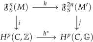
anomaly. I showed in the sections above that fictitious internal circular spaces may induce artificial discrete symmetries. These concepts have a direct analogy in the domain of (co)homology with torsion coefficient groups. In categorical terms, the connection between the construction using auxiliary fields and the construction using torsion coefficient groups can be written as the following commuting diagram:
Here,
is the space of physical solutions of the theory containing an initial number
n of fields while
is the space of physical solutions for the theory obtained via the introduction of new auxiliary fields such that the required internal “circular” space emerges. This space contains the required topological particularity introduced via the employment of the auxiliary fields. It must be specified that the morphism in the lower arrow requires the use of the universal coefficient theorem. The upper arrow morphism is valid when we talk about the physical domain of the theory.
is a torsion group, e.g.,
. If
and/or
are being taken into account in the construction of the respective spaces, the horizontal arrows become isomorphisms.
Simply stated, if we have a module M over a ring R, an element is called a torsion element of the module if there exists a regular element (not a zero divisor) such that . In the case of a group G, an element is called a torsion element of the group if it has finite order, i.e., if there is a positive integer m such that , e being the element of G. A (sub)-group is called torsion (sub)-group (or circular or periodic) if all of its elements are torsion elements. Examples are -groups with p-prime.
In this section, I briefly introduce the Atiyah–Singer index theorem in the context of the Hodge–de-Rham theory. This is being done following mainly [
39]. I also construct an analogy between the method presented above and the cohomology with coefficients in groups with torsion. By using the isomorphism between the de-Rham cohomology group and the group of harmonic functions (
,
) over a closed manifold, I introduce the general form for index theorems, i.e., a connection between an index calculated in a topological, respectively an analytical, fashion. The presence of torsion in the coefficient structure of the cohomology, while preserving the isomorphism between cohomology and the group of harmonic functions (a result of the second Hodge theorem), also reflects the effect of an “internal circular space” as presented in the previous section from the perspective of index theorems. As I will show in what follows, different choices of coefficient groups may merge or dissociate classes in the cohomology groups. Due to the isomorphism with the group of harmonic forms, the same effect will be found on the analytic side of the index theorems. The universal coefficient theorems assure us that the choice of a rather unusual coefficient group has no physical effects if the
and/or
groups are correctly considered in the chain complex. For this, I follow my previous result regarding the relativity of anomalies [
14]. For the sake of completeness, I state here the following:
Theorem 1 (The universal coefficient theorem [
14,
18])
. If C is a chain complex of free abelian groups, then there are natural short exact sequences:∀n, G, and these sequences split. Here, is the torsion group associated with the homology. In this way, homology with arbitrary coefficients can be described in terms of homology with the “universal” coefficient group . For cohomology, the exact sequence changes into:Here, is the group extension. Relevant for the situation at hand is the following.
Example 1 (Homotopy and coefficient group [
14,
18])
. Take a Moore space obtained from by attaching a cell by a map of degree m. The quotient map induces trivial homomorphisms on the reduced homology with coefficients since the nonzero reduced homology groups of X and occur in different dimensions. However, with coefficients, the situation changes, as we can see considering the long exact sequence of the pair , which contains the segment:Exactness requires that is injective, hence non-zero, since is , the cellular boundary map:being exactly:One can see that a map can have induced maps that are trivial for homology with coefficients, but not so for homology with coefficients for suitably chosen m. This means that homology with coefficients can tell us that f is not homotopic to a constant map, information that would remain invisible if one used only coefficients. This relatively simple example shows that torsion coefficient groups are in some sense “measuring devices” that allow us to consistently take into account global properties without inconsistencies.
Following [
14], it is precisely the
correction that has an important effect on the presence of a sign ambiguity (an
anomaly). It is relevant at this point to remember that because on a compact Riemannian orientable manifold
M, the cohomology group
is isomorphic to the group of harmonic forms on
M,
, the two groups have the same dimension, hence:
where
is the Betti number of
M.
We can define the exterior derivative
d and the co-differential
as adjoint to each other. On the ring of differential forms,
on
M the action of
d induces a sequence:
The co-differential generates another sequence of arrows oriented this time in the opposite direction:
We now have:
Neither of these sequences is exact, i.e.,
and similarly for
. However,
or equivalently
. This means that the first sequence is a de-Rham complex. To this complex, we can associate the de-Rham cohomology groups, which measure the lack of exactness of the sequence:
We define
to be co-closed (resp. co-exact) if
(resp.
. We also can define the homogeneous Hodge–de-Rham operator
. We then obtain on
:
Lets now assume that the
-form
can be expressed as
,
. If this is so, the product
is zero. Proceeding as in the previous section where the Hodge decomposition has been introduced, we conclude that:
or, in other words, that
has a unique splitting of the form:
and consequently, since
, we have:
where
is a harmonic
i-form
. Every
i-th de-Rham cohomology class is represented by one and only one harmonic form:
If the analytic index of the de-Rham complex is now the integer defined by the alternating sum:
we find:
Here,
is the Euler class of the tangent bundle to
M. The right-hand side of this expression is of a topological nature: it is a topological index. If
M is odd-dimensional,
since
. This remains true for index theorems of other differential operators. We may note that
and
have the same kernel (a harmonic form is closed and co-closed). Let us split:
into even and odd forms:
Let
and
be the operators defined by:
Then,
D is a mapping:
defined as:
Its adjoint
is a mapping:
The associated Laplacians are given by:
Thus, we can replace the definition of the analytical index of the de-Rham complex by:
or equivalently by:
since:
In fact,
(resp.
) is the orthogonal complement of
(resp.
). We also have that:
and hence, the analytic index may be given as:
The form of the analytic index for the de-Rham complex is not specific to this case. To see what it has in common with the index theorem for other complexes, let us look at its general structure. First, we notice that the de-Rham sequence should have been written:
where
is the module of cross-sections of the vector bundle
since the differential
i-forms of
may be regarded as sections of the vector bundle
. The writing of the above sequence requires the existence of a differential operator of degree one acting on a sequence of sections of vector bundles
such that
. With this, the sequence qualifies as a complex.
Secondly, the fact that the expression:
was a well-defined one was guaranteed by the nature of the Laplacian operator
, the kernel of which is finite dimensional. This is a consequence of the fact that
is an elliptic operator.
An elliptic operator defined on a compact manifold has a finite-dimensional kernel and co-kernel, and expressions of the type:
are well defined for them.
Looking at the de-Rham complex on the compact boundaryless manifold M, we conclude that it is an elliptic complex since its associated Laplacians are elliptic. Let E be a vector bundle. An elliptic complex is a finite sequence of differential operators acting on smooth sections, such that , and the Laplacians of the complex , where is the adjoint operator with respect to the scalar product on the fibres with a smooth density on M, are elliptic on .
Since
, it follows that if the complex
is elliptic, so is the complex
where the arrows point in the opposite direction. To relate this picture to the form of the index for a de-Rham complex, we have to reduce the elliptic complex to a two-term elliptic complex (to roll up the complex) and see that the new complex has the same index as the original one
. This is where the comparison with the previous equations for the index comes in. Defining the even and odd bundles
,
:
and the associated Laplacian:
The analytical index of an elliptic complex
is defined to be the integer:
We note that the differential operator defining a complex, the Riemannian scalar product defining its adjoint and the ellipticity property, which guarantees that the rhs of the equation above is well defined (an integer), are the ingredients for the definition of an index of a compact manifold. In order to have a non-trivial index, the operator D cannot be self-adjoint. The Atiyah–Singer index theorem states that the analytic index is equal to the topological index of the complex, which is given by the rhs in the formula of the Atiyah–Singer index theorem. The statement of this theorem is as follows:
Let
be an elliptic complex over a compact boundaryless manifold
M of even dimension
n. Then, the index of the complex is given by:
is the Todd class of the complexified tangent bundle
and
is the Euler class. In the above integrand, only
n-forms are retained. If the manifold is odd-dimensional, the index of the differential operator
D is zero. Due to this trivial situation, it makes sense to go to an even-dimensional field-space as explained in the BRST-dual-BRST construction of the previous sections.
At this moment, we can see how the main construction of this article affects the Atiyah–Singer theorem. The next splitting due to the Kahler structure introduced over the field space gives:
The isomorphism between the cohomology group and the group of harmonic forms is preserved. The introduction of a Kahler structure over the field space has two effects. First, it allows the construction of an explicit internal circular space and second; it allows a different splitting, one that dissociates the two different signs that can arise when a large gauge transformation is performed. We can repeat the same discussion as above, only this time with a non-trivial coefficient structure in cohomology. In fact, one can choose the torsion of the coefficient groups in cohomology such that they compensate precisely the topological properties of the
group. If, for example, the coefficient group in cohomology is
, the two regions of positive and negative eigenvalues that make the path integral associated with the
problem inconsistent become properly separated. The coefficient group in cohomology now contains different classes. The isomorphism between the cohomology group and the group of harmonic forms on
M was until now understood as:
The universal coefficient theorem assures us that we can use a different coefficient group. One choice then is:
This choice can be used such that the distinction between the two regions of different signs is made explicit. Let us now take the dimension of the above construction. As the isomorphism is preserved, the dimensions of the two groups will be the same, albeit different from the case above. Indeed:
The introduction of inner space circular integration paths is translated in coefficient groups in cohomology. This leads to a reorganization of the integration such that, simply stated,
where
represent points on the non-trivial manifold where the integration is performed in the two cases (with trivial coefficient group and with
coefficient group). If the first subset on the right is characterized by a positive sign and the second by a negative sign, then the specific choice of a torsional (periodic) coefficient group in cohomology makes the two domains clearly separated and well indexed. I explained in the Introduction of this article the origin of the Bose–Einstein and Fermi–Dirac statistics as a result of how the topology of the quotient space
where
is the symmetry group changes with respect to the original space
X. While the two spaces remain isomorphic, the global properties differ according to the number of dimensions considered. It is interesting to see how it is possible to relate the case with
to the case
. Indeed, in dimensions larger than two, performing two rotations around a singularity brings us to a curve that can be homotopically deformed into a point. However, the integration is sensible to homology and cohomology. In principle, the homology groups
of a chain complex
C relate to the shape of the manifold. The cohomology groups
relate to the differential forms defined over a manifold. Hence, if we have a manifold
M characterized by a sequence of homology groups, then one can define the integral:
as being characterized by the differential form
and by the manifold
M. Integration can be seen as the pairing:
such that:
where this pairing is constructed with real coefficients and this coefficient structure characterizes also the measure of integration and implicitly the differential form
. Here,
represents a class in homology, and
represents a class in cohomology. The pairing above is an isomorphism only when this particular choice of coefficients is made. For other coefficients, this pairing may fail to be an isomorphism, the correction being controlled by the
and
groups. The pairing then becomes:
The same principle translates for functional integration in the partition function. Because of this, the case for
is anomalous only if certain unsuitable choices of coefficient groups in (co)homology are made. Otherwise, the integration (which is seen as a pairing between (co)homology) is itself defined via a torsion coefficient group, which acts as an “anti-anomaly”. The physical aspects of the original theory are however preserved, in the
group, albeit not in an explicit way.