An Intelligent Fishery Detection Method Based on Cross-Domain Image Feature Fusion

Abstract

Target detection technology plays a crucial role in fishery ecological monitoring, fishery diversity research, and intelligent aquaculture. Deep learning, with its distinct advantages, provides significant convenience to the fishery industry. However, it still faces various challenges in practical applications, such as significant differences in image species and image blurring. To address these issues, this study proposes a multi-scale, multi-level, and multi-stage cross-domain feature fusion model. In order to train the model more effectively, a new data set called Fish52 (multi-scene fish data set, a data set containing 52 fish species) was constructed, on which the model achieved an mAP (mean average precision is a key measure of model performance) of 82.57%. Furthermore, we compared prevalent one-stage and two-stage detection methods on the Lahatan (single-scene fish data set) and Fish30 data set (a data set containing 30 fish species) and tested them on the F4k (Fish4Knowledge (F4K) is a data set focused on fish detection and identification) and FishNet data set (it is a data set containing 94,532 images from 17,357 aquatic species). The mAP of our proposed model on the Fish30, Lahatan, F4k, and FishNet data sets reaches 91.72%, 98.7%, 88.6%, and 81.5%, respectively, outperforming existing mainstream models. Comprehensive empirical analysis indicates that our model possesses a high generalization ability and reaches advanced performance levels. In this study, the depth of the model backbone is deepened, a novel neck structure is proposed, and a new module is embedded therein. To enhance the fusion ability of the model, a new attention mechanism module is introduced. In addition, in the adaptive decoupling detection head module, introducing classes with independent parameters and regression adapters reduces interaction between different tasks. The proposed model can better monitor fishery resources and enhance aquaculture efficiency. It not only provides an effective approach for fish detection but also has certain reference significance for the identification of similar targets in other environments and offers assistance for the construction of smart fisheries and digital fisheries.

1. Introduction

In recent years, deep learning, target detection, and other technologies have gone deep into various fields, but the technology has not been well applied in the field of fishery detection, fishery ecological monitoring, fishery diversity research, and intelligent aquaculture, and other related fields urgently need the support of target detection and other technologies. Fish object detection technology aims to distinguish and locate fish in images or videos in multiple scenes and is the technical core of the automatic monitoring of fish growth status [1]. 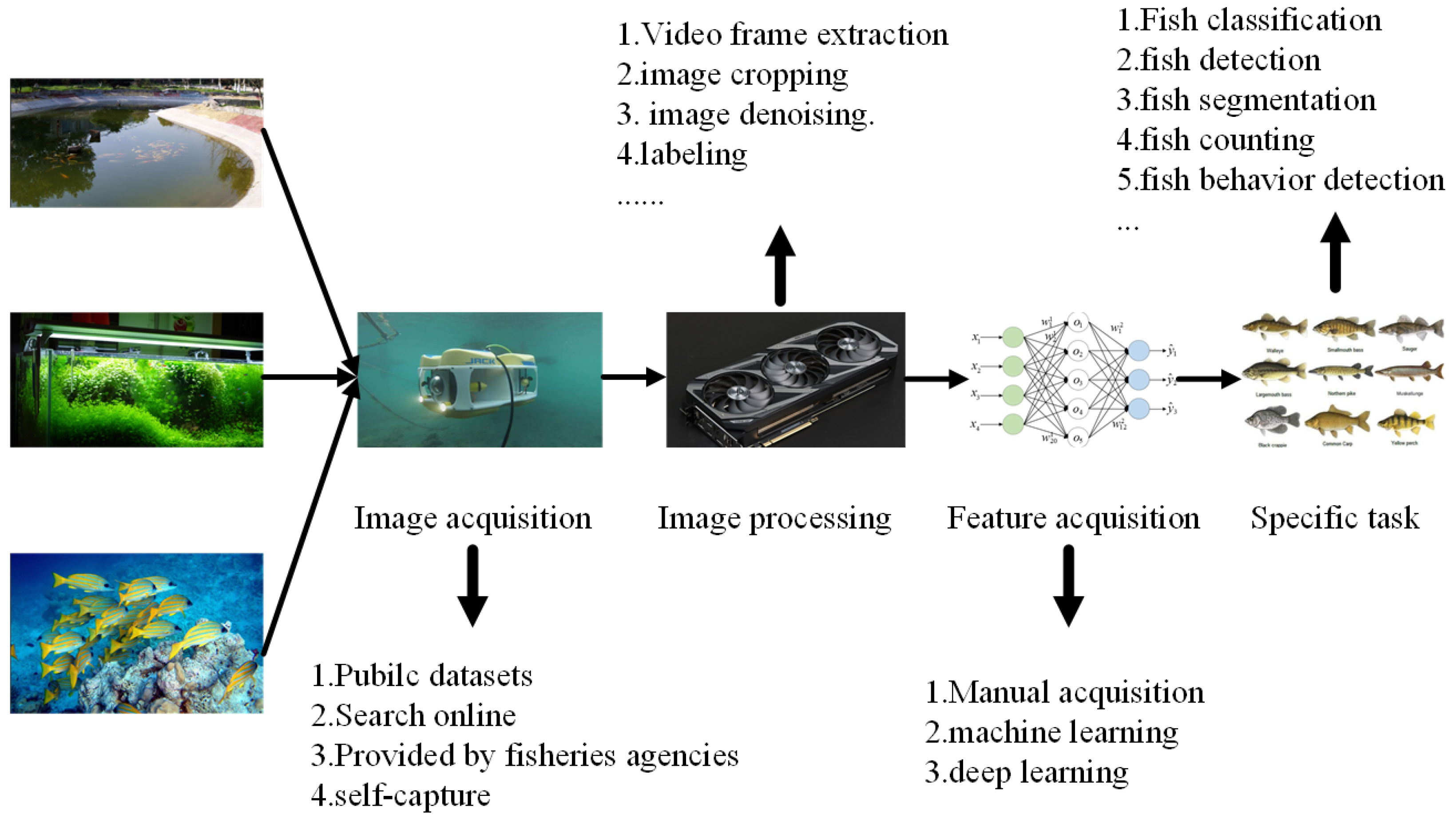At the same time, assessing fish species diversity and monitoring changes in aquatic species are also key tasks of related research [2]. In addition, the technology can monitor fish species in an intelligent way to achieve the protection of fish diversity, and low-cost, high-performance, high-precision fish detection technology that has almost no adverse impact on the living environment of fish has become the basis for fish behavior analysis and growth state measurement. At present, the main research process in this field is shown in Figure 1 below. Firstly, image and video data are obtained from various scenarios, followed by data processing, feature extraction, and model training to achieve specific downstream tasks so as to realize research in specific fields, and then the intelligent perception, identification, and classification of fish species and quantity are realized so as to effectively prevent illegal overfishing. The sustainable development of fishery resources is protected and the fishery intelligence of the whole industry chain is realized.

Combining many factors, such as model size, detection speed, and deployment difficulty, we proposed a multi-scale, multi-level, multi-stage cross-domain feature fusion discrimination model TMFD (triple the multi-scale/multi-layer/multi-stage fish detection) based on fish data images in different scenes. In view of the large differences in size and color of fish in multi-scene images, we deepened the depth of the model from the original three layers to the current five layers. Secondly, in the neck stage, in order to reduce the loss of a large number of high-dimensional features caused by direct use of the 1*1 convolution between the backbone and neck, we introduce the MCB (multiple convolution batch normalization) module to segment the depth features through splitting, and then obtain a new output through the convolution operation using the output on one side as the residual edge. The other side repeats the above work as a new input. After several splits, the final output is concat spliced to further obtain a unified output channel. At the same time, in the neck stage, a comparison of FPN [3], PANet [4], BiFPN [5], and our neck structure MMCFPN (multi-stage, multi-level and cross-domain) is proposed, and the DBMFormer (DPConv combines binary additive attention with MLP Former) attention mechanism is added after multi-level feature splicing in the first stage, which effectively utilizes the feature information of different channels in the same spatial position. The feature interaction between different stages and different levels is realized, and the feature information at all levels is efficiently integrated, which further enhances the detection effect of the model and improves the discriminability of the whole model. Finally, in order to avoid the mutual influence of the required features among different subtasks, we completely decouple the three subtasks of classification, positioning, and regression, which further improves the detection results of the model.

Our contributions are as follows:

• In this paper, a novel multi-scale, multi-level, and multi-stage cross-domain feature fusion discrimination model TMFD is proposed to detect fish targets in different scenarios, thus effectively preventing illegal overfishing.
• The multi-layer segmentation residual fusion module MCB and a new neck structure MMCFPN are introduced to solve the problem of multi-channel deep features losing a large amount of feature information when the number of feature channels is unified. At the same time, multi-scale, multi-level, and multi-stage features are integrated across domains, improving the feature integration ability of the model.
• In the neck fusion process of the model, we introduce DBMFormer, a Q and K binary fusion attention mechanism, which further processes the fused features, strengthens the features, and thus improves the detection ability.

The remaining sections of this article are structured as follows: Section 3 provides a description of the pertinent materials and data sets utilized in our study. In Section 4, we present our approach, also referred to as the model. It begins by introducing the overall model and subsequently elaborates on the relevant technical modules and innovations employed. Additionally, it outlines the loss function used. Moving on to Section 5, we introduce our specific experiments, encompassing experiment details, and demonstrate the superiority of our model through comparative experiments, ablation experiments, and visualizations. Section 6 delves into discussing challenges encountered in current research work along with future research directions. Finally, in Section 7, we conclude by summarizing the relevant findings from this study.

2. Related Work

With the further development of fishery intelligence, fish classification, segmentation, target detection, and other related tasks have gradually introduced deep learning, which can automatically extract more abundant features from massive information and can constantly learn the difference between the actual value and the predicted value according to the needs. In the early stage of fishery resource target detection, machine learning is mainly relied on, which can effectively classify and locate fish targets and provide key data for related industries. As a reliable and economical technology, machine learning has the advantages of non-contact monitoring, a wide application range, and long-term stable operation [6]. Lee et al. [7] used the global shape matching method to further identify fish by testing descriptors such as Fourier, polygon approximation, and line segments, achieving an accuracy of more than 90% for four species in aquariums. Fouad MM et al. [8] used feature extraction techniques based on scale invariant feature transform (SIFT) and accelerated robust feature (SURF) algorithms in combination with support vector machines (SVMs) to automatically classify Nile tilapia, which was superior to other machine learning techniques, such as artificial neural networks (ANNs) and the K-nearest neighbor (K-CNN) algorithm. Spampinato et al. [9] improved the fish detection effect by combining local feature extraction, patch coding, and pooling operations with the background modeling method of multi-scale feature aggregation in the later stage. Ravanbakhsh et al. [10] used an automated method for fish detection based on a shape-based level set framework to model the shape of fish through principal component analysis (PCA) to achieve the detection of fish. In previous relevant studies [11,12], the texture, color, shape, and other local features of the target were manually designed and selected through appropriate feature extraction algorithms to ensure that the selected features could accurately represent different objects. However, the characteristics selected by this method rely too much on manual techniques, and the characteristics depend on human subjective judgment, which has a great influence on the final detection. At the same time, in addition to the traditional manual monitoring methods, there are also sense-based [13] and acoustic [14] methods. However, due to the large differences in different scenes and complex environment, the layout of sensors and acoustic methods is difficult, the cost is high, and the efficiency is low, so it is difficult to further study and develop. Therefore, the traditional fish target detection algorithm that relies on machine learning cannot meet the needs of the actual situation.

At present, the two-stage object detection algorithm is applied to the fishery scene. The first stage is to classify the foreground and background in the image and screen out the candidate frame from a large number of anchor frames; the second stage is to adjust the position of the candidate frame and classify the objects in the candidate frame. Rauf et al. [15] further deepened the network on the basis of VGG and used deep convolutional neural networks to realize the automatic recognition of fish based on visual features. Maløy et al. [16] proposed a two-flow cyclic network (DSRN) based on deep learning by integrating spatial networks and 3D convolutional motion networks to automatically capture the spatiotemporal behavior of salmon during swimming. Manda et al. [17] first introduced Faster RCNN into the field of fish detection and achieved an accuracy rate of 82.4% on the data set of remote underwater video stations. Labao et al. [18] used numerous convolutional networks on the basis of RPN, connected them through long- and short-term memory networks and cascading structures, and introduced an automatic correction mechanism to further improve the detection accuracy of the model. Salman et al. [19] used a region-based convolutional neural network to detect freely moving fish in an unconstrained underwater environment. They used background subtraction and optical flow to make use of the fish movement information in the video, and then combined the results with the original images to generate corresponding candidate regions to further improve the effect of the model. Liu et al. [20] improved the Faster RCNN by embedding a convolutional kernel adaptive selection unit in the backbone to enhance the feature extraction capability of the network and solve the detection problem of small densely distributed benthic creatures under overlapping and occlusion images. Peng et al. [21] proposed a two-stage detection network named S-FPN that added a fast connection structure to FPN and proposed a new segmented focal length loss (PFL) function to reduce the interference of a large number of unrelated background samples, thereby improving the detection of objects at different scales. Although the two-stage algorithm has high detection accuracy, its reasoning speed is slow, and it needs to occupy many resources, so it cannot be well deployed on edge devices.

Compared with the two-stage algorithm, the first-stage algorithm has been vigorously developed because of characteristics such as its faster reasoning speed, lower resource occupation, and easy deployment. For application scenarios requiring detection speed, the first-stage detector is more suitable. It does not have the stage of classifying the foreground and background, but directly generates the classification probability and positioning coordinate value of the target in one stage, determines the positioning and classification of the predicted object according to the grid unit where the central point of the object is located, and then directly regresses the classification probability and positioning coordinates of the target to achieve the prediction effect. Wang et al. [22] proposed that, by improving the up-sampling operator based on the YOLOV5 model, problems such as a small detection target and fuzzy detection can be effectively solved. Based on YOLOV3, Wei et al. [23] added an SE attention module to learn the relationship between channels, enhance the semantic information of depth features, and enhance the detection effect of small targets. Jalal et al. [2] combined the optical flow and Gaussian mixture model with YOLO, eliminating the problem that YOLO was initially only used to capture static and clearly visible fish targets, and expanding the detection range. Wageeh et al. [24] used the multi-scale Retinex algorithm to enhance the cloudy underwater image, and then used YOLO combined with the optical flow algorithm to detect fish and obtain the activity trajectories of fish. Hu et al. [25] used YOLOV3-Lite to improve the blocking and loss functions of fish schools so as to better identify fish behaviors. Yu et al. [26] extracted fish contour features based on the attentional full convolutional instance segmentation network (CAM-Decoupled SOLO), and combined pixel position information with a channel attention mechanism to realize the fusion of target position information and channel dimension information. Zhao et al. [27] made improvements to YOLOV4, replacing the original backbone with MobileNetV3 and standard convolution with deep separable convolution, thus achieving a significant reduction in network parameters and computation. Kandimalla et al. [28] integrated the Norfair tracking algorithm with YOLOv4 to track fish in video data, thus improving the effect of fish detection. Wang et al. [29] improved YOLOV5 by adding multilevel features, adding feature mapping, and adding a SiamRPN structure to detect and track target fish. Yu et al. [30] designed a novel multi-attention path aggregation network named APAN that combines coordinate competing attention and spatial supplementary attention and a double-transmission underwater image enhancement algorithm to further enhance the detection effect of the model. Xu et al. [31] proposed a new refined marine object detector based on the attention spatial pyramid pool network (SA-SPPN) and bidirectional feature fusion strategy to detect fine marine objects. Jia et al. [32] proposed a new marine organism target detection model EfficientDet-Reved (EDR) that reconstructs MBConvBlock by adding a channel shuffle module to realize information exchange between the channel of the element layer. Xu et al. [33] proposed a new scale perception feature pyramid structure SA-FPN in order to enrich the semantic features of prediction and further improve the marine target detection performance. In order to further improve the detection accuracy of underwater fish in complex underwater environments, Liu et al. [34] proposed a dual-path (DP) pyramid vision converter (PVT) feature extraction network DP-FishNET. The model enhances the ability of extracting global and local features from underwater images and enhances the feature reusability. The detection system proposed by Dharshana et al. [35] based on the YOLO framework focuses on changes in fish scales and location and looks for distinguishing traits to distinguish fish.

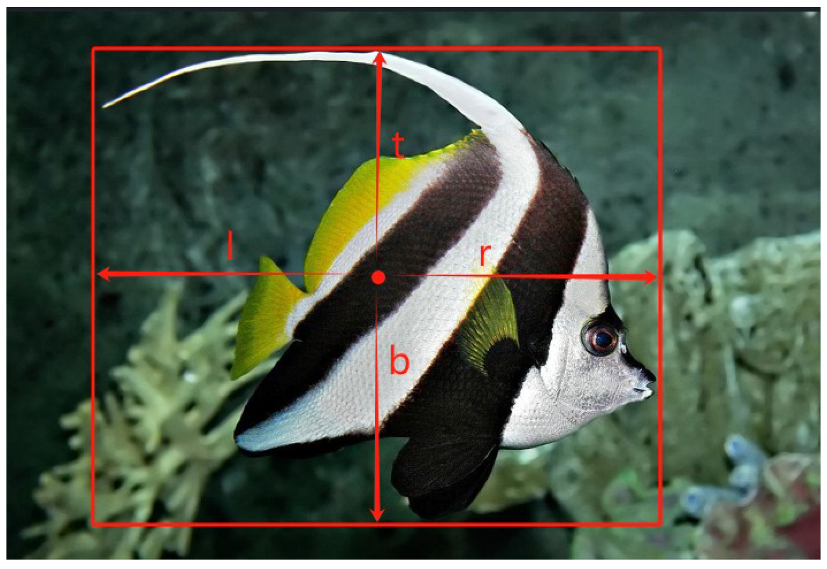
Whether it is a one-stage algorithm or a two-stage algorithm, it predicts the category of the target and the center point offset and then obtains the actual prediction results based on the anchor frame, but there are some problems in this approach, such as how to find the appropriate size of the anchor frame, how to allocate positive and negative samples, how to choose different anchor frames, and so on. In order to solve the above problems, our model abandoned the traditional idea of an anchor frame and directly predicted the distance of the point to the left (l: left), upper (t: top), right (r: right), and lower (b: bottom) sides of the target in each position of the prediction feature map; this idea is not only simple but also more effective, as shown in Figure 2.

Our model is similar to the FCOS model, which simplifies the process of target detection through the design of no anchor points. Combined with the relevant data in

Table 1. Effectiveness of multiple models on multiple data sets.

Model	Backbone	mAP (Different Data Sets)
		Fish30	Lahatan	Fish52	f4k	FishNet
Centernet	Resnet50	48.17	69	52.2	74.1	62.5
Efficientdet	Efficientnet	87.65	63.75	62.82	79.3	68.7
Faster-rcnn	Resnet50	80.37	74.6	50.4	84.6	74.3
Fcos	Resnet50	81.14	91.43	72.56	84.9	72.6
Retinanet	Retinanet	60.41	93.77	69.28	73.9	69.8
SSD	Resnet50	62.01	93.19	74.96	77.2	73.1
Yolov3	Darknet	75.31	75.24	53.68	88.4	79.6
Yolov4	Cspdarknet	62.4	74.82	52.08	88.9	77.4
Yolov5	Cspdarknet	81	92.54	58.12	91.7	77.3
Yolov7	Cspdarknet	86.23	85.35	50.75	95.6	84.2
YoloX	Cspdarknet	89.64	92.17	62.68	90.2	80.6
MambaVision	ViT	88.32	90.12	76.52	94.8	75.3
Inception-Yolo	Inception	90.5	91.8	73.42	93.1	80.6
TMFD(ours)	ResNet50	91.72	98.7	86.57	96.2	78.3

, it can be found that, compared with the traditional method with anchor points, our model has a better effect than other models when the proportion of data sets is unchanged. At the same time, through a series of innovative mechanisms, it achieves high precision target detection. Specifically, there are these points:

• The anchor-free design of the model avoids the complex calculation and hyperparameter setting related to the anchor frame, reduces the computation and memory consumption, and thus improves the generalization ability of the model.
• The model adopts a full convolutional network, which can process input images of any size without clipping or scaling the images, thus improving the adaptability of the model.
• The model realizes target detection and positioning by predicting the distance between each pixel point and the target boundary box. This pixel-level prediction method improves the accuracy of the target boundary box.
• A new “center-ness” branch is introduced to predict the deviation between pixels and the corresponding bounding box center, which is used to reduce the proportion of low-quality detection bounding boxes and improve the detection accuracy.

3. Materials

At present, there are few fish data sets in multiple scenarios, most of which are data in a single scenario, such as the underwater image data set (UTDAC) [4], natural light underwater exploration data set (RUOD) [5], DeepFish [36], LifeCLEF [37], FishNet [38], etc. The relevant information of specific relevant data sets is shown in

Table 2. Summary of fishery detection-related data sets.

Data Set	Labels	Data Set Size
A-UTDAC	Species name	5168 images labeled with detection frames for testing and 1293 images for validation.
B-RUOD	Species name	A total of 90,310 images in 74 categories labeled with detection frames.
C-DeepFish	Fish/no fish	40 k classification labels, 3.2 k images with point-level annotations, 310 segmentation masks.
D-LifeCLEF2015	Species name	∼1000 annotated videos.
E-SUIM	Object name	∼500 annotated images in semantic segmentation mask.
F-Fish4knowledge	Fish/no fish	3.5 k bounding boxes.
G-Fish30	Species name	A total of 7000+ images labeled with categories and detection frames.
H-Fish52	Species name	A total of 12,200+ images labeled with categories and detection frames.
I-Lahtan	Species name	A total of 9600+ sheets labeled with categories and detection frames.

.

There is much relevant data, but various data sets are more or less flawed, such as DeepFish and Fish4Knowledge data sets, where the data size is large enough, but the label is not specific to fish categories but fish; the UTDAC, LifeCLEF, and SUIM data sets, which are also large enough to be labeled according to specific fish categories, but only have 4, 10, or 8 different species, with fewer target species, and cannot provide good classification results. Fish in the seagrass habitats data set meet the previous requirements, but its scenario is too simple and not the best choice. The above mentioned relevant data represent the legend in Figure 3.

Our data set comes from a wide range of sources. By searching online resources or cooperating with fishery agencies to obtain public data sets, we adopted a self-production method to construct a training set by adding labels to fish images of different species and different scenarios for data enhancement processing. Specific data sets can be used for model training and performance verification, and the data set contains fish images in multiple scenarios, with diversity and complexity. Fish images also include images with no fish targets and only partial fish targets. To add labels to fish images, the fish in the image is selected by using the smallest rectangular box, and then the distance between the center point of the smallest rectangular box and the four sides is marked as the position mark of the fish image, and the category of fish in the image is marked. Data enhancement is used to process each image by means of flipping, scaling, random noise, color transformation, Mosaic, etc., to improve the generalization ability of the model and reduce the overfitting probability. These data sets provide rich samples for model training.

A total of three data sets were used in our experiment, namely Fish30, Fish52, and Lahatan. Fish30 is the key data set of our experiment, and its data distribution is shown in Figure 4. Data sets Fish52 and Lahatan are mainly used for comparative experiments to verify the effect of our model. These data sets are faced with such challenges as blurred pixels, too high a similarity between the foreground and background, fish species diversity, occlusion, a large difference in target size, etc. However, they also make up for the shortcomings of the aforementioned data sets. In order to further improve the quality of the data set, improve the training effect of the model, reduce the probability of overfitting, and improve the generalization ability of the model, we carried out a series of data enhancement operations on the data set, such as flipping, scaling, random noise, color transformation, Mosaic, etc.

4. Method

4.1. Overall Model

We used multiple target detection models to test on the Fish30 data set and found that conventional general target detection algorithms were not effective on specific data sets. After comprehensive experiments on detection algorithms such as Faster RCNN, EfficientDet, Yolov3, and Yolov4, relevant experimental data are shown in Table 1.

Our model eliminates predefined anchor boxes, avoids complex computations associated with anchor boxes, such as computational overlap during training, and significantly reduces training memory. The structure consists of three parts, and the backbone structure obtains the main features of the model. We use ResNeXt as the backbone for several reasons:

• ResNeXt has good advantages in feature extraction capability, computational efficiency, and model performance compared with other models (such as VGG, GoogLeNet, etc.).
• ResNeXt continues the idea of stacking the same modules in VGG, ResNet, and other networks and using shortcut, which can make the network training deep and control the number of hyperparameters at the same time.
• Apply the split-transform-merge strategy in Inception inside the module; that is, first use 1 × 1 convolution to split the input to a lower dimension, then perform feature mapping, and finally merge the results.

We used the neck structure to enhance the features and the detection head to realize recognition, classification, and regression. The specific model structure is shown in Figure 5. When an image is input into the model, it is first extracted by a deepened backbone to better detect targets with size differences. Since the conventional extension will cause the deep module to have a large number of channels, which is not conducive to the reduction in the number of subsequent channels, we started to reduce the expansion of the number of channels at the entrance of the backbone. At the connection between the backbone and neck, we initially used 1*1 convolution to reduce the number of channels, but we found that such an operation will cause the model to lose too many features. For this reason, we designed an MCB module, which largely solves this problem. At the neck, we constructed a new MMCFPN structure. In order to further reduce the loss of image features between different stages and levels, we fused the features between different levels in different stages, used conventional convolution for down-sampling, and used bilinear interpolation for up-sampling. After the first stage of feature fusion, we added the DBMFormer attention module to enhance the feature information of different channels in the same spatial location. Finally, in the head phase, we improved the detect head of the original model and completely decoupled classification, center-ness, and regression, which helped to reduce the interaction between the three tasks.

4.2. Improvement Points and Related Technical Descriptions

4.2.1. Multi-Level and Multi-Stage Residual Feature Fusion Neck

In view of the large differences in features of different scales and the changes in the multi-scale imaging of image targets, we improved the neck structure of the model and conducted progressive tests to finally obtain our MMCFPN model structure, as shown in Figure 6 for specific details. Specifically, our neck structure is a change from the earlier FPN structure. It gradually evolved through PANet and BiFPN structures. C3, C4, C5, C6, C7, respectively, represent feature maps of different scales after the backbone’s output, corresponding to the backbone’s output of Layer3, Layer4, Layer5, Layer6, Layer7. Generally speaking, the deeper the convolutional layer, the larger the corresponding receptive field, the lower the resolution of the feature map, and the more important the semantic feature extraction ability. In order to combine high-resolution features (lower layer) and strong semantic features (upper layer), the FPN structure connects the features output from different layers top-down and horizontally. However, the single-stage up-sampling operation only makes the lower layer features obtain the upper layer semantic information, while the upper layer does not obtain the corresponding lower layer information. The PANet structure solves this problem by adding a bottom-up stage to the FPN structure. At the same time, a new problem arises. Due to multiple up- and down-sampling operations and layer feature transmission, the model loses part of the feature information, and the current layer structure only obtains the features of adjacent stages and layer structures, which still have certain limitations. The BiFPN structure is improved on this basis; in order to reduce the loss of features, it merges more features without adding too much additional computation, and introduces additional edges between the original input and output nodes, which, to some extent, compensates for this problem.

Our structure is influenced by the previous one, and, in order to further obtain richer feature information, we not only extend the multi-stage up- and down-sampling operations but also introduce feature information of different stages, as well as information of different layers, which enhances the multi-scale feature extraction capability of the network. At the time of up-sampling, they are up-sampled to the same scale by bilinear interpolation. In the final feature fusion stage, our structure introduces the upper and lower hierarchical features from the previous stage together while down-sampling, which greatly enhances the model fusion of the more differentiated feature information, further strengthens the feature extraction ability of the model, and thus improves the discriminative ability of the whole model, which is formulated as in (1).

$$\begin{array}{cc}\hfill P_6^{out}& =Conv6\left[downsample\right(Conv5(\dots ))\hfill \\ \hfill & +P6rrr\hfill \\ \hfill & +upsample\left(P7rrr\right)\hfill \\ \hfill & +downsample\left(p5rrr\right)]\hfill \end{array}$$

(1)

Combined with the MMCFPN structure in Figure 6, $p_6^{out}$ represents the output result of line 6, which has undergone a 3*3 convolution (Conv6())with stride = 1. The input of the convolution is the result of the addition of features from the previous layers, and P6rrr is the direct input structure with the same size without any operation. P7rrr is a deep layer structure of the previous stage that needs to undergo an up-sampling operation to achieve the same size structure. P5rrr is a shallow layer structure of the previous stage and needs to undergo a down-sampling operation to achieve the same size structure. A single r represents the output of the trunk after passing through the convolutional layer; two r’s represent the convolution fusion result of the up-sampled depth feature and the previous feature. Similarly, three r’s represent the result of subsequent multi-stage, multi-level integration.

4.2.2. Multi-Level Segmentation Residual Module (MCB)

The five feature layers output by the backbone have different heights, widths, and channel numbers. However, in order to facilitate cross-domain fusion operations at different levels and stages in the MMCFPN stage, we need to adjust the channel number of feature maps output by the backbone at different stages to be consistent. We find that if 1*1 convolution is directly used, it can cause the model to lose many deep features, such as the backbone obtaining channels of the feature layer through the last layer to reach 4096. In order to facilitate subsequent fusion operations, we set the number of channels before fusion to 256, and directly use 1*1 convolution to change 4096 to 256, which will greatly reduce the accuracy of the model. Relevant data are shown in

Table 3. Experimental data used to verify the validity of the location of the module.

Model	${\mathit{mAP}}_{\mathbf{50}}$	${\mathit{mAP}}_{\mathbf{75}}$	${\mathit{mAP}}_{\mathbf{50}\mathbf{:}\mathbf{95}}$
Baseline (FCOS)	81.14	80.6	72.9
FCOS + MMCFPN(Me)	89.78	88.6	80.6
Me + Conv + CSP	71.97	70.16	63.9
Me + CSP	88.99	87.36	79.8
Me + Conv + C2f	71.24	70.12	63.62
Me + C2f	78.16	76.9	70.1
Me + Conv + MCB	71.79	70.2	66.5
Me + MCB	90.81	88.92	81.4
Me + DBMFormer	90.05	89.25	82.6

. To solve this problem, we introduce the MCB module, which captures local details and global context information by the parallel processing of different scale feature maps. By using different processing strategies in different branches, the MCB module can re-calibrate features to adapt to different scale feature representation. In addition, the MCB module uses residual connection technology to ensure that the original information is preserved during the feature fusion process to avoid the problem of gradient disappearance in the deep network. Finally, in order to reduce the computational load, the MCB module adopts deep separable convolution to reduce the parameter and computational cost while maintaining the feature representation capability. The specific model structure is shown in Figure 7.

4.2.3. DBMFormer

Although traditional self-attention mechanisms can capture long-distance dependencies, their computational complexity increases square (O($n^2$)) as the length of the input sequence increases, resulting in a decrease in the efficiency of the model. To solve this problem, the DBMFormer module replaces the traditional self-attention mechanism, which is designed to improve the performance of deep learning models in fish detection tasks and address the limitations of the traditional self-attention mechanism. The improvements are as follows:

• Enhanced feature fusion: A single convolutional model can no longer meet the requirements of detection scenarios. Through innovative structural design, DBMFormer realizes the deep fusion of features at different scales and levels to improve the model’s understanding of complex data and capture more detailed feature differences.
• Solves the problem of information loss: Through the two-branch structure and multi-head attention design, the problem of model information loss is reduced.
• Optimizes computing efficiency: By optimizing the structure and parameter settings, the consumption of computing resources is reduced while maintaining the performance.
• Improvement of attention mechanism: Through the attention mechanism, the model can focus on key areas in the image adaptively, reducing the problem of a poor effect caused by the target occupying different proportions and positions in the image.

A Q and K binary fusion attention mechanism is introduced that effectively replaces quadratic matrix multiplication with linear element multiplication. Additive attention eliminates the need for expensive matrix multiplication operations, significantly reducing the computational complexity of the model, resulting in more efficient contextual information capture and superior speed–accuracy tradeoffs. Our DBMFormer improves the traditional self-attention module by using simple and effective Conv, which makes the local and global representation more consistent. The specific structure of the module is shown in Figure 8. After the pre-fusion, the features first go through the DPConv module, composed of 3*3 deep convolution and 3*3 point convolution. Further learning of spatial information and encoding of local representations are carried out. Then, through the binary additive attention module, the original features are divided into query and key, and the context information on each scale of the input size is further learned by random weighting. Finally, the output feature maps are fed into a linear block consisting of two 1*1 point-by-point convolution layers, batch normalization, and GeLU functions to generate nonlinear features. The formula is described as follows:

$$\widehat{x_i}=x_i+Conv2d\left(Conv2d\left(DWConv\left(x_i\right)\right)\right)$$

(2)

$$\widehat{x_i}=QK\left(\widehat{x_i}\right)+\widehat{x_i}$$

(3)

$${\widehat{x}}_{i+1}=Dropout\left(Conv2d\left(Con{v}_{N,C,G,D}\left({\widehat{x}}_i\right)\right)\right)$$

(4)

where QK denotes the DBMFormer attention module and $Con{v}_{\mathrm{N},\mathrm{C},\mathrm{G},\mathrm{D}}$ denote batch normalization, normal convolution, GeLu, and Dropout in that order.

Through the operation of the module, the model can capture the morphological differences between different fish species. Through the multi-branch structure, the DBMFormer module can effectively process multi-scale information for fish detection of different sizes. The design of the module is an important innovation of the traditional self-attention mechanism that not only improves the performance of the model in fish detection tasks but also improves the performance of the model. The efficiency of the model is also improved by reducing the computational complexity.

4.2.4. Fully Decoupled Detection Head

When the output is determined, the decoupling detection head operation is performed first. While this makes computation difficult, it also improves detection performance and convergence speed. Second, the network uses anchor-less operation to better detect by reducing parameters, and the detection head predicts classification and positioning information from the feature map after feature fusion. The two tasks do not focus on functionality in the same way [39]. The classification task focuses more on the similarity between the extracted element class and the known element class. The location task focuses on the location information of the detection frame. The decoupling head uses different feature graphs to decouple the classification and positioning tasks, thus speeding up the convergence of the model. However, a good detection head should focus on objects of different sizes, different positions, and different tasks; in other words, it should be more spatially aware and mission-aware.

For the classification branch, the score of the corresponding data set category is predicted at each position in the prediction feature map. For the regression branch, four distance parameters are predicted at each position of the predicted feature map (distance l from the left of the target, distance t from the upper side, distance r from the right side, and distance b from the lower side; note that the values predicted here are relative to the feature map scale). Suppose that the coordinate of a point on the prediction feature map back to the original map is ($C_x$, $C_y$), and the step distance of the feature map relative to the original map is s; then, the target boundary frame coordinate corresponding to the point predicted by the network is

$$X_{min}=C_x-l·s,Y_{min}=C_y-t·s$$

(5)

$$X_{max}=C_x+r·s,Y_{max}=C_y+b·s$$

(6)

For the center-ness branch, one parameter will be predicted at each position of the prediction feature map. Center-ness reflects the distance between this point (a certain point on the feature map) and the target center, and its range is between 0 and 1. The closer it is to the target center, the closer it is to 1. Here is the formula for calculating the center-ness true label (only the positive sample is considered when calculating the loss, i.e., the predicted point is within the target).

$$centernes{s}^{*}=\sqrt{{\displaystyle \frac{min(l^{*},r^{*})}{max(l^{*},r^{*})}}\times {\displaystyle \frac{min(t^{*},b^{*})}{max(t^{*},b^{*})}}}$$

(7)

When selecting high-quality Bboxes in the network post-processing part, the predicted target class score and center-ness will be multiplied and then rooted. Then, the Bboxes will be sorted according to the obtained results, and only the Bboxes with higher scores will be retained. The goal is to screen out Bboxes that have a low target class score and are far from the target center, leaving only high-quality Bboxes.

4.3. Loss Functions

Our model head has three output branches, and the corresponding loss function (LOSS) is also divided into three parts, which are loss of classification ($L_{cls}$), loss of localization ($L_{reg}$), and loss of center-ness ($L_{ctrness}$), and calculated as follows.

$$\begin{array}{cc}\hfill L(P_{x,y},t_{x,y},s_{x,y})& ={\displaystyle \frac{1}{N_{pos}}}\sum _{x,y}{L}_{cls}(P_{x,y},c_{x,y}^{*})\hfill \\ \hfill & +{\displaystyle \frac{1}{N_{pos}}}\sum _{x,y}{l}_{(c_{x,y}^{*}>0)}{L}_{reg}(t_{x,y},t_{x,y}^{*})\hfill \\ \hfill & +{\displaystyle \frac{1}{N_{pos}}}\sum _{x,y}{l}_{(c_{x,y}^{*}>0)}{L}_{ctrness}(s_{x,y},s_{x,y}^{*})\hfill \end{array}$$

(8)

Here is an explanation of the relevant parameters in Equation:

• $P_{x,y}$ denotes the predicted score of each category at the point of the feature map (x,y).
• $c_{x,y}^{*}$ denotes the true category label corresponding to the point at the feature map (x,y).
• l($c_{x,y}^{*}$>0) is 1 if it is matched as a positive sample at point (x,y) of the feature map, and 0 otherwise.
• $t_{x,y}$ denotes the information of the predicted target bounding box at the point of feature map (x,y).
• $t_{x,y}^{*}$ denotes the information of the real target bounding box corresponding to the point at the feature map (x,y).
• $s_{x,y}$ denotes the predicted center-ness at the point of feature map (x,y).
• $s_{x,y}^{*}$ denotes the true center-ness at the point corresponding to the feature map (x,y) point.

For classification loss $L_{cls}$, bce_focal loss is used, i.e., binary cross-entropy loss with focal loss, and all samples are involved in the calculation (positive and negative samples) when calculating the loss. For localization loss $L_{reg}$, iou_loss is used, where only positive samples are involved in the computation of the loss. Center-ness loss is used as binary cross-entropy loss, where only positive samples are involved in the computation of the loss. The expression for BCE_loss is shown in Equation (9).

$$BCE(\widehat{n},n)=-\widehat{n}log\left(n\right)-(1-\widehat{n})log(1-n)$$

(9)

In the process of matching positive and negative samples, it is better to obtain the GT information $c_{x,y}^{*}$ and $t_{x,y}^{*}$ corresponding to the points of the feature map (x,y); as long as the match is to a certain GT target, then $c_{x,y}^{*}$ corresponds to the category of the GT, and $t_{x,y}^{*}$ corresponds to the bbox of the GT. It is a little more complicated to obtain the true center-ness ($s_{x,y}^{*}$), which is calculated as in the previous Equation (8). The loss that we use in this process is the GIoU loss, whose equation is shown in (10). The equation of GIOU is shown in (11).

$$L_{GIoU}=1-GIoU(0\le L_{GIoU}\le 2)$$

(10)

$$GIoU=IoU-{\displaystyle \frac{A^c-u}{A^c}}(-1\le GIoU\le 1)$$

(11)

• IoU denotes the ratio of the intersection and concatenation of the predicted and true bounding boxes, respectively;
• the $A^c$ denotes the area of the rectangle containing both the true bounding box (green) and the predicted bounding box (red);
• the u denotes the area of the concatenation of the true and predicted bounding boxes.

4.4. Positive and Negative Sample Matching Algorithm

Before calculating the loss, we need to match positive and negative samples. In the anchor-based target detection network, the IoU of each anchor box and each GT are generally matched by calculating the IoU threshold set in advance. For example, if the IoU of an anchor box and a GT is greater than 0.7, we will set the anchor box as a positive sample. However, for anchor-free networks, there is no anchor at all. For a certain point (x,y) on the feature map, as long as it falls into the central region of the GT box and satisfies that point (x,y) is within the sub-box range of ($C_x-rs$, $C_y-rs$, $C_x+rs$, $C_y+rs$), where ($C_x$, $C_y$) is the central point of GT, s is the step distance between the feature map and the original image, and r is the distance from the center of GT controlled by a hyperparameter, then it is regarded as a positive sample. In other words, the point (x,y) must not only be within the range of GT but also close enough to the central point of GT ($C_x$, $C_y$) to be regarded as a positive sample.

5. Experiment

5.1. Experimental Details and Procedures

The software and hardware environment used in our experiment is NVIDIA CUDA 20.04, Ubuntu 20.2 system, Nvidia 4090 graphics card, 16 GB memory. The model is trained using the stochastic gradient descent (SGD) optimization algorithm, the parameters can be updated once for each piece of data, and the update of each epoch parameter is consistent with the number of samples. It randomly selects each sample, and the order of updating each epoch sample is also random, dynamically adjusting the learning rate of each parameter. The specific model training process steps are as follows.

First, the data are divided into a training set and verification set according to a certain proportion, and some pre-processing operations are carried out on the data set. Then, through the generator function, the batch size batch_size is set to 16. Through the form of a data stream, 16 samples are extracted from the training samples each time to participate in the training. The initial learning rate (learning_rate) is set to 0.001, and the total training epoch is set to 100. Each time, batch_size samples are extracted from memory through the generator to participate in a parameter update of gradient descent. The model training parameter values are shown in

Table 4. Parameters used in the training process.

Parameters	Value
epoches	300
batch-size	16
num-classes	30
strides	[8, 16, 32, 64, 128]
Input_size	[640, 640]
Init_lr	le-2
Min_lr	Init_lr * 0.01
Optimizer_type	sgd
momentum	0.9
weight-decay	0
Lr_decay_type	cos

. At the same time, the weights corresponding to the training are taken as the final parameters of the model. After that, the neural network obtains the predicted value through forward propagation, calculates the error between the predicted value and the actual value, and terminates the training iteration if the error meets the threshold set by the system. Otherwise, training is continued until the maximum number of training rounds set by the system is reached, and the training is stopped.

To ensure the consistency of our model’s performance under different conditions, we conducted additional experiments. As the nature of the data set is inherent, no changes were made to it. However, further testing was carried out by adjusting model parameters such as batch size, input size, and epoch. Our experimental results indicate that reducing these three parameters leads to a decrease in mAP, while increasing them also results in a corresponding decrease in mAP. Our analysis reveals that setting a too large batch size reduces the number of gradient updates and slows down the convergence of the model. Moreover, large batch sizes may cause overfitting and diminish the generalization ability of the model. Conversely, smaller batch size settings reduce computational efficiency, increase training time, and make the convergence process of the model unstable. The specific experimental data are presented in

Table 5. The results of different parameter training are compared.

Epoches	Batch Size	Input_Size	mAP
300	16	[640, 640]	91.72
300	16	[320, 320]	88.2
300	8	[640, 640]	90.6
200	16	[640, 640]	89.4
200	16	[320, 320]	85.7
200	8	[640, 640]	83.9

.

5.2. Evaluation Index

AP values are often used to measure the recognition performance of target detection models. The value is between 0 and 1, and the greater the value, the higher the recognition accuracy of the model. The precision (P) and recall (R) integrals are calculated as follows:

$$AP={\int }_0^{1}P\left(R\right)dR$$

(12)

In our experiment, in order to measure the detection effect of the model on fish more comprehensively, three different mAP values, namely $mA{P}_{50}$, $mA{P}_{75}$, and $mA{P}_{50:95}$, were used. The subscript is used to specify the IoU threshold for the intersection area between the real tag box and the prediction box. If the IoU of $mA{P}_{50}$ and $mA{P}_{75}$ is 0.5 and 0.75, refer to the mAP value, respectively. $mA{P}_{50:95}$ is the average of the ten values of $A{P}_{50}$, $A{P}_{55}$, $A{P}_{60}$, …, $A{P}_{95}$. The calculation formula is as follows. In addition, recall, precision, and F1 score were also used to evaluate the effect of the model, where TP is the number of positive samples correctly predicted, FP is the number of positive samples incorrectly predicted, FN is the number of negative samples incorrectly predicted, C is the number of detection classes, and AP is the average accuracy. A recall is defined as the proportion of errant fish correctly detected in the total number of errant fish in the sample. Precision represents the proportion of fish with correct abnormal behavior detected out of all fish with abnormal behavior detected.

$$A{P}_{50:95}={\displaystyle \frac{1}{10}}(A{P}_{50}+A{P}_{55}+A{P}_{60}+\dots +A{P}_{95})$$

(13)

$$Recall=TP/(TP+FN)$$

(14)

$$Precision=TP/(TP+FP)$$

(15)

$$F1=(2\ast Recall\ast Precision)/(Recall+Precision)$$

(16)

$$mAP={\displaystyle \frac{{\sum }_{c=1}^{C}AP\left(c\right)}{C}}$$

(17)

5.3. Contrast Experiment

In order to determine which model is more suitable for the detection of this scenario, we found some recently popular target detection methods and tested them on the Fish30 data set. Relevant data are shown in Table 1. We found that there are still large differences among different models on the Fish30 data set. With the improvement of the YOLO series model, its effect has also been improved, and this problem is also reflected in the Lahatan2022 and Fish52 data sets. In the Lahatan2022 data set, only Yolov5 and YolovX are slightly higher than the basic model FCOS, while, in the Fish52 data set, only YOLOV5 and YOLOVX are slightly higher than the basic model FCOS. Only the model SSD is higher than the base model FCOS. From the comparison results of these three data sets and multiple models, it can be found that our model has the best effect. On the one hand, our analysis is because the YOLO series model only integrates three layers of features in the neck stage, while we integrate five layers of features. On the other hand, our newly added module has a corresponding effect. At the same time, in order to further prove the generalization ability of the model, we added some work contents and conducted further experiments on open data sets such as F4k and FishNet. According to the experimental results, the Yolo series model is better than the basic model FCOS as a whole, and our model is better than the Yolo series model to a certain extent. It also further proves the excellent generalization ability of our model.

5.4. Ablation Experiment

In order to analyze the effectiveness of the modules proposed in this paper, this subsection details the ablation experiments conducted based on the Fish30 data set, whose results are shown in

Table 6. Data from ablation experiments to validate the effectiveness of the module.

Model	${\mathit{mAP}}_{\mathbf{50}}$	${\mathit{mAP}}_{\mathbf{75}}$	${\mathit{mAP}}_{\mathbf{50}\mathbf{:}\mathbf{95}}$
Baseline(FCOS)	81.14	80.6	72.9
FCOS + PANet	86.96	86.7	78.9
FCOS + BiFNet	88.73	87.63	79.4
FCOS + MMCFPN(Me)	89.78	88.6	80.6
Me + CSP	88.99	87.36	79.8
Me + C2f	78.16	76.9	70.1
Me + CA	80.09	78.84	71.6
Me + ECA	74.27	73.16	66.72
Me + MCB	90.81	88.92	81.4
Me + DBMFormer	90.05	89.25	82.6
Me + MCB + DBMFormer	91.72	90.8	83.7

. We used the FCOS model as a benchmark for our experiments on the Fish30 data set, and its result reached 81.14%; after that, we tested FPN, PANet, BiFPN, and our MMCFPN, and the effectiveness of the models were improved, and our model even reached 89.78%. After that, we also added the CSP and C2f modules, which are common in the YOLO series of models, for testing, and the effects were reduced. With the addition of our MCB module, the effect of the model is 9.67% higher than that of the baseline, and 1.03% higher than that of the model with the addition of the MMCFPN structure, which is enough to prove that our module greatly reduces the problem of feature loss in the process of realizing the backbone to the neck. In addition, in the neck, in order to better integrate the multi-scale features of different levels and stages across domains, we added the DBMFormer module on top of the MMCFPN module, and the result reached 90.05, which is 8.91% higher than the baseline and 0.27% higher than that of the model with the MMCFPN structure. Finally, the final result of our model after improving the overall structure and adding MCB and DBMFormer modules reached 91.72%. The data related to the data set in our experiment are the real data distribution obtained through our statistical calculation, and all the results of the experiment are obtained according to the relevant parameters of other people’s models rather than directly quoting the relevant data in other people’s articles.

When adding different modules, it is also worth considering where to add modules. To this end, we also conducted relevant experiments to find the most suitable location, and the relevant experimental data are shown in Table 3. Taking CSP as an example, the Conv + CSP structure is used at the connection between the backbone and neck. First, 1*1 convolution is used to adjust the number of different channels output by different layers of the backbone to be consistent, and then the CSP module is used. For only CSP, 1*1 convolution is avoided and the CSP module is directly used. The features of different numbers of channels output by different layers of the backbone are taken as inputs, and the features of the same number of channels are directly output by other modules, which confirms that the direct use of modules has the best effect.

5.5. Detection Process and Result Visualization

In order to better display the knowledge learned by each module during the training process, we selected part of the middle-layer structure of the model for visualization, which helps us to analyze the corresponding features learned by the network at a specific layer, and analyzed whether the network has learned the correct features or information by focusing on the area of the network in turn. The corresponding feature diagram of some feature layers is shown in Figure 9. Since there are many stages and levels of the model, we took out several representatives of the lower layers as follows: A represents features that are outputted by the backbone’s first layer of convolution just after images enter the model; B represents features that are outputted by the backbone’s layer1 completely; C represents features that are outputted by the MCB module; D represents features that are outputted by an image after the first fusion operation; E represents the features of the image output after the DBMFormer module; and F represents the features of the image after the second fusion.

We can find that, with the gradual deepening of the model, the image features that can be seen by the naked eye are gradually blurred, the features concerned by the model are getting deeper and deeper, and the fused features are gradually increasing. In the detection stage, in order to facilitate the understanding of the special areas concerned by the model to identify the target, we drew the corresponding heat map, as shown in Figure 10. In addition, in order to further understand the focus of the model during detection, we used gradient-weighted category activation mapping (Grad-CAM) technology to draw the heat map on several detection images, which helps us to analyze the specific areas that the network pays more attention to for a certain category, and then helps us to improve the model and display the map according to the effect. We can find that the focus of the model is more at the central point of the target, which is just in line with the construction principle of our model, proving the effectiveness of the model.

By comparing the visual detection results, Figure 11 visually shows the effectiveness of this algorithm in target detection tasks (when the IoU threshold is 0.5). According to the detection results of different comparison algorithms, it can be seen that when only the model trained in the source domain is used to identify fish in the new domain, the baseline model Faster RCNN cannot effectively identify and locate the target. The generalization performance of the traditional target detection algorithm is poor in the face of domain deviation caused by data distribution difference. However, the proposed method can pay more attention to the individual to be measured so as to obtain a better generalization performance under different complex and changeable cross-domain conditions and scenarios.

5.6. Other Experimental Results

In order to further illustrate the effect of the model, we conducted tests on the Fish30 data set and randomly recorded the results of several indicators, such as precision, recall, and F1 score. Due to the large number of models involved in the comparison, we chose a more common and excellent model: a single-stage detection method YoloV5 and a two-stage detection method Faster RCNN are compared in precision, recall, and F1 score. It can be seen from the

Table 7. Precison, recall, and F1 score results for our model on the Fish30 data set.

Model	Class	Precision	Recall	F1-Score
YoloV5	Abramis brama	95.24	83.33	0.89
	Blicca bjoerkna	57.89	64.71	0.61
	Carassius gibelio	77.78	56.00	0.65
	Cyprinus carpio	88.52	93.10	0.91
	Esox lucius	94.74	81.82	0.88
	Gobio gobio	86.36	73.08	0.79
	Leuciscus cephalus	80.00	72.73	0.76
	Leuciscus idus	87.5	65.62	0.75
Faster RCNN	Abramis brama	95.24	83.33	0.89
	Blicca bjoerkna	57.89	64.71	0.61
	Carassius gibelio	77.78	56.00	0.65
	Cyprinus carpio	88.52	93.10	0.91
	Esox lucius	94.74	81.82	0.88
	Gobio gobio	86.36	73.08	0.79
	Leuciscus cephalus	80.00	72.73	0.76
	Leuciscus idus	87.5	65.62	0.75
Our model	Abramis brama	92.59	96.15	0.94
	Blicca bjoerkna	83.33	95.24	0.89
	Carassius gibelio	82.14	100	0.90
	Cyprinus carpio	98.44	98.44	0.98
	Esox lucius	92.68	97.44	0.95
	Gobio gobio	85.71	75.00	0.8
	Leuciscus cephalus	96.43	90.00	0.93
	Leuciscus idus	85.42	93.18	0.89

that the highlighted data are more reflected in our model, which further proves the superiority of the model. In addition, the mAP corresponding to its related models is shown in Figure 12, which also reflects the superiority of our model.

6. Discussions

With the increase in population, land resources cannot meet the needs of human beings, and marine resources are vital to human beings. When marine resources are exploited, excessive human behavior can disturb the marine environment and reduce the efficiency of operations.The automatic operation of underwater detection equipment such as AUVs is conducive to the rational exploitation, research, and protection of marine living resources. Currently, the research in this field is still facing many problems in data sets, models, and applications. At the same time, there are many research directions in this field that can improve the current situation, and the following aspects are mainly discussed here:

• Data set: Firstly, there are fewer fishery-related multi-scene fish data sets at present, and most of them are single-scene data; secondly, a large amount of image information is extracted from video frames at present, but drawing corresponding labeling information for these images is also a tricky problem; lastly, the scene of this type of data set is highly dynamic, and how to filter the noise contained in the images is a major difficulty. In the future, improvements can be made on the basis of existing techniques to minimize manually labeled features and expand the number of training data sets, such as pre-detection using the existing model weights and then filtering by hand.
• Model: Improving the generalization ability of the model is one of the most difficult tasks in fishery detection, i.e., how to reduce the difference between the model effect on the training set and the test set, and the task is even more difficult in the special scenario of specific fish detection. In the future, model-related techniques such as migration learning, weakly supervised learning, and knowledge distillation can be used for enhancement, using migration learning techniques to avoid re-training the model on a new data set and to obtain the optimal value of the weights at the time of migration; using weakly supervised learning techniques to reduce the use of samples with labels; and using knowledge distillation techniques to reduce the parameters of the model and make the model more lightweight.
• Application: The “intelligent fishery” has penetrated into all aspects of the marine industry chain, regarding how to further develop the specific “fish detection” task in the “intelligent fishery” and how to integrate big data analytics, remote control, remote monitoring, and data management. How to further integrate big data analysis, remote control, aquaculture methods, and the intelligent Internet of Things is also a major difficulty. In the future, classification, detection, segmentation, counting, and other tasks can be integrated to establish an intelligent analysis platform based on fishing catches so as to achieve the intelligent sensing of fishery catches and forecasting of fishing grounds.

Overall, research related to fishery resources is still at an early stage and still faces many problems, but there are many related research areas. In the future, it is important to explore and develop more effective cross-domain adaptive algorithms, to mine more domain-invariant information, to further improve the accuracy of cross-domain detection, to embed the proposed method into an intelligent fish detection system in order to quickly adapt to the fish detection tasks in different scenarios so as to make the intelligent detection equipment more rapid and versatile, and to enable the relevant practitioners to obtain the categories of the relevant species within a certain area in order to guide the subsequent related work; therefore, this study has strong practicality.

7. Conclusions

In this paper, we propose a multi-scale, multi-level, multi-stage cross-domain feature fusion discriminative model TMFD (triple the multi-scale/multi-layer/multi-stage fish detection) for fish detection in multi-scenarios. Specifically, the model extends the three output channels of the FCOS model backbone, and, in order to minimize the loss of a large number of features from the backbone output after 1*1 convolution, the MCB (multiple convolution batch normalization) module is added at the connection. Meanwhile, in order to enhance the extraction ability of non-rigid fish with multi-scale and multi-pose changes, we propose our MMCFPN (multi-stage, multi-level, and cross-domain feature pyramid network) structure in the neck part, which not only extends the multi-stage up and down sampling operation but also introduces the feature information of different stages, as well as the information of different layers, which, in turn, enhances the network discriminability. In the neck fusion process of the model, we introduce a Q and K binary fusion attention mechanism, DBMFormer (DPConv combines binary additive attention with MLP Former), which further processes the features after fusion and strengthens the features. In addition, in the detection head part, in order to avoid mutual interference among classification, localization, and regression tasks, we decouple the three sub-tasks so that they independently complete their corresponding feature tasks. The excellent target detection of our model is demonstrated by comparison and ablation experiments on multiple data sets, which show that good performance can be obtained in new target domains without any additional labeling. The proposed algorithm is shown to outperform similar models through a series of experiments on multiple data sets from different scenarios, indicating that the proposed algorithm is beneficial for assessing fish species diversity and aquaculture as well as other fishery activities. In addition, it contributes to ecological monitoring and marine biodiversity studies. In the future, the model can be further designed toward being lightweight while maintaining detection accuracy and integrating multiple tasks, such as classification, detection, segmentation, and counting, to establish an intelligent analysis platform based on fishing catch to achieve the intelligent sensing of fishery catch and fishery forecast, which can then be applied to a wider range of fields.

References

1. Salman, A.; Maqbool, S.; Khan, A.H.; Jalal, A.; Shafait, F. Real-time fish detection in complex backgrounds using probabilistic background modelling. Ecol. Inform. 2019, 51, 44–51. [Google Scholar] [CrossRef]
2. Jalal, A.; Salman, A.; Mian, A.; Shortis, M.; Shafait, F. Fish detection and species classification in underwater environments using deep learning with temporal information. Ecol. Inform. 2020, 57, 101088. [Google Scholar] [CrossRef]
3. Liu, S.; Qi, L.; Qin, H.; Shi, J.; Jia, J. Path aggregation network for instance segmentation. In Proceedings of the IEEE Conference on Computer Vision and Pattern Recognition, Salt Lake City, UT, USA, 18–22 June 2018; pp. 8759–8768. [Google Scholar]
4. Tan, M.; Pang, R.; Le, Q.V. Efficientdet: Scalable and efficient object detection. In Proceedings of the IEEE/CVF Conference on Computer Vision and Pattern Recognition, Seattle, DC, USA, 14–19 June 2020; pp. 10781–10790. [Google Scholar]
5. Fu, C.; Liu, R.; Fan, X.; Chen, P.; Fu, H.; Yuan, W.; Zhu, M.; Luo, Z. Rethinking general underwater object detection: Datasets, challenges, and solutions. Neurocomputing 2023, 517, 243–256. [Google Scholar] [CrossRef]
6. Dong, C.Z.; Catbas, F.N. A review of computer vision–based structural health monitoring at local and global levels. Struct. Health Monit. 2021, 20, 692–743. [Google Scholar] [CrossRef]
7. Lee, D.J.; Schoenberger, R.B.; Shiozawa, D.; Xu, X.; Zhan, P. Contour matching for a fish recognition and migration-monitoring system. In Two-and Three-Dimensional Vision Systems for Inspection, Control, and Metrology II; SPIE—The International Society for Optical Engineering: Bellingham, DC, USA, 2004; Volume 5606, pp. 37–48. [Google Scholar]
8. Fouad, M.M.; Zawbaa, H.M.; El-Bendary, N.; Hassanien, A.E. Automatic nile tilapia fish classification approach using machine learning techniques. In Proceedings of the 13th International Conference on Hybrid Intelligent Systems (HIS 2013), Gammarth, Tunisia, 4–6 December 2013; pp. 173–178. [Google Scholar]
9. Spampinato, C.; Palazzo, S.; Joall, P.H.; Paris, S.; Glotin, H.; Blanc, K.; Lingr, D.; Precioso, F. Fine-grained object recognition in underwater visual data. Multimed. Tools Appl. 2016, 75, 1701–1720. [Google Scholar] [CrossRef]
10. Ravanbakhsh, M.; Shortis, M.R.; Shafait, F.; Mian, A.; Harvey, E.S.; Seager, J.W. Automated Fish Detection in Underwater Images Using Shape-Based Level Sets. Photogramm. Rec. 2015, 30, 46–62. [Google Scholar] [CrossRef]
11. Hu, X.; Liu, Y.; Zhao, Z.; Liu, J.; Yang, X.; Sun, C.; Chen, S.; Li, B.; Zhou, C. Real-time detection of uneaten feed pellets in underwater images for aquaculture using an improved YOLO-V4 network. Comput. Electron. Agric. 2021, 185, 106135. [Google Scholar] [CrossRef]
12. Lin, J.Y.; Tsai, H.L.; Lyu, W.H. An integrated wireless multi-sensor system for monitoring the water quality of aquaculture. Sensors 2021, 21, 8179. [Google Scholar] [CrossRef]
13. Manicacci, F.M.; Mourier, J.; Babatounde, C.; Garcia, J.; Broutta, M.; Gualtieri, J.S.; Aiello, A. A wireless autonomous real-time underwater acoustic positioning system. Sensors 2022, 22, 8208. [Google Scholar] [CrossRef]
14. Rauf, H.T.; Lali, M.I.; Zahoor, S.; Shah, S.Z.; Rehman, A.U.; Bukhari, S.A. Visual features based automated identification of fish species using deep convolutional neural networks. Comput. Electron. Agric. 2019, 167, 105075. [Google Scholar] [CrossRef]
15. Måløy, H.; Aamodt, A.; Misimi, E. A spatio-temporal recurrent network for salmon feeding action recognition from underwater videos in aquaculture. Comput. Electron. Agric. 2019, 167, 105087. [Google Scholar] [CrossRef]
16. Mandal, R.; Connolly, R.M.; Schlacher, T.A.; Stantic, B. Assessing fish abundance from underwater video using deep neural networks. In Proceedings of the 2018 International Joint Conference on Neural Networks (IJCNN), Rio de Janeiro, Brazil, 8–13 July 2018; pp. 1–6. [Google Scholar]
17. Labao, A.B.; Naval, P.C., Jr. Cascaded deep network systems with linked ensemble components for underwater fish detection in the wild. Ecol. Inform. 2019, 52, 103–121. [Google Scholar] [CrossRef]
18. Salman, A.; Siddiqui, S.A.; Shafait, F.; Mian, A.; Shortis, M.R.; Khurshid, K.; Ulges, A.; Schwanecke, U. Automatic fish detection in underwater videos by a deep neural network-based hybrid motion learning system. ICES J. Mar. Sci. 2020, 77, 1295–1307. [Google Scholar] [CrossRef]
19. Liu, Y.; Wang, S. A quantitative detection algorithm based on improved faster R-CNN for marine benthos. Ecol. Inform. 2021, 61, 101228. [Google Scholar] [CrossRef]
20. Peng, F.; Miao, Z.; Li, F.; Li, Z. S-FPN: A shortcut feature pyramid network for sea cucumber detection in underwater images. Expert Syst. Appl. 2021, 182, 115306. [Google Scholar] [CrossRef]
21. Wang, H.; Zhang, S.; Zhao, S.; Lu, J.; Wang, Y.; Li, D.; Zhao, R. Fast detection of cannibalism behavior of juvenile fish based on deep learning. Comput. Electron. Agric. 2022, 198, 107033. [Google Scholar] [CrossRef]
22. Wei, X.; Yu, L.; Tian, S.; Feng, P.; Ning, X. Underwater target detection with an attention mechanism and improved scale. Multimed. Tools Appl. 2021, 80, 33747–33761. [Google Scholar] [CrossRef]
23. Wageeh, Y.; Mohamed, H.E.; Fadl, A.; Anas, O.; ElMasry, N.; Nabil, A.; Atia, A. YOLO fish detection with Euclidean tracking in fish farms. J. Ambient. Intell. Humaniz. Comput. 2021, 12, 5–12. [Google Scholar] [CrossRef]
24. Hu, J.; Zhao, D.; Zhang, Y.; Zhou, C.; Chen, W. Real-time nondestructive fish behavior detecting in mixed polyculture system using deep-learning and low-cost devices. Expert Syst. Appl. 2021, 178, 115051. [Google Scholar] [CrossRef]
25. Yu, X.; Wang, Y.; Liu, J.; Wang, J.; An, D.; Wei, Y. Non-contact weight estimation system for fish based on instance segmentation. Expert Syst. Appl. 2022, 210, 118403. [Google Scholar] [CrossRef]
26. Zhao, S.; Zhang, S.; Lu, J.; Wang, H.; Feng, Y.; Shi, C.; Li, D.; Zhao, R. A lightweight dead fish detection method based on deformable convolution and YOLOV4. Comput. Electron. Agric. 2022, 198, 107098. [Google Scholar] [CrossRef]
27. Kandimalla, V.; Richard, M.; Smith, F.; Quirion, J.; Torgo, L.; Whidden, C. Automated detection, classification and counting of fish in fish passages with deep learning. Front. Mar. Sci. 2022, 8, 823173. [Google Scholar] [CrossRef]
28. Wang, H.; Zhang, S.; Zhao, S.; Wang, Q.; Li, D.; Zhao, R. Real-time detection and tracking of fish abnormal behavior based on improved YOLOV5 and SiamRPN++. Comput. Electron. Agric. 2022, 192, 106512. [Google Scholar] [CrossRef]
29. Yu, H.; Li, X.; Feng, Y.; Han, S. Multiple attentional path aggregation network for marine object detection. Appl. Intell. 2023, 53, 2434–2451. [Google Scholar] [CrossRef]
30. Xu, F.; Wang, H.; Sun, X.; Fu, X. Refined marine object detector with attention-based spatial pyramid pooling networks and bidirectional feature fusion strategy. Neural Comput. Appl. 2022, 34, 14881–14894. [Google Scholar] [CrossRef]
31. Jia, J.; Fu, M.; Liu, X.; Zheng, B. Underwater object detection based on improved efficientdet. Remote. Sens. 2022, 14, 4487. [Google Scholar] [CrossRef]
32. Xu, F.; Wang, H.; Peng, J.; Fu, X. Scale-aware feature pyramid architecture for marine object detection. Neural Comput. Appl. 2021, 33, 3637–3653. [Google Scholar] [CrossRef]
33. Lin, T.Y.; Dollár, P.; Girshick, R.; He, K.; Hariharan, B.; Belongie, S. Feature pyramid networks for object detection. In Proceedings of the IEEE Conference on Computer Vision and Pattern Recognition, Honolulu, HI, USA, 21–26 July 2017; pp. 2117–2125. [Google Scholar]
34. Liu, Y.; An, D.; Ren, Y.; Zhao, J.; Zhang, C.; Cheng, J.; Liu, J.; Wei, Y. DP-FishNet: Dual-path Pyramid Vision Transformer-based underwater fish detection network. Expert Syst. Appl. 2024, 238, 122018. [Google Scholar] [CrossRef]
35. Dharshana, D.; Natarajan, B.; Bhuvaneswari, R.; Husain, S.S. A novel approach for detection and classification of fish species. In Proceedings of the 2023 Second International Conference on Electrical, Electronics, Information and Communication Technologies (ICEEICT), Trichirappalli, India, 5–7 April 2023; pp. 1–7. [Google Scholar]
36. Qin, H.; Li, X.; Liang, J.; Peng, Y.; Zhang, C. DeepFish: Accurate underwater live fish recognition with a deep architecture. Neurocomputing 2016, 187, 49–58. [Google Scholar] [CrossRef]
37. Joly, A.; Goëau, H.; Glotin, H.; Spampinato, C.; Bonnet, P.; Vellinga, W.P.; Planqué, R.; Rauber, A.; Palazzo, S.; Fisher, B.; et al. LifeCLEF 2015: Multimedia life species identification challenges. In Proceedings of the Experimental IR Meets Multilinguality, Multimodality, and Interaction: 6th International Conference of the CLEF Association, CLEF’15, Toulouse, France, 8–11 September 2015; Proceedings 6 2015. Springer: Berlin/Heidelberg, Germany; pp. 462–483. [Google Scholar]
38. Khan, F.F.; Li, X.; Temple, A.J.; Elhoseiny, M. FishNet: A Large-scale Dataset and Benchmark for Fish Recognition, Detection, and Functional Trait Prediction. In Proceedings of the 2023 IEEE/CVF International Conference on Computer Vision (ICCV), Paris, France, 4–6 October 2023; pp. 20439–20449. [Google Scholar] [CrossRef]
39. Jooshin, H.K.; Nangir, M.; Seyedarabi, H. Inception-YOLO: Computational cost and accuracy improvement of the YOLOv5 model based on employing modified CSP, SPPF, and inception modules. IET Image Process 2024, 18, 1985–1999. [Google Scholar] [CrossRef]
Figure 1. Fisheries intelligence research process.
Fishes 09 00338 g001
Figure 2. Detection method based on detecting the center point of the target.
Fishes 09 00338 g002
Figure 3. Data set related images (AI).
Fishes 09 00338 g003
Figure 4. Fish30 data set category distribution.
Fishes 09 00338 g004
Figure 5. Overall structure of the model.
Fishes 09 00338 g005
Figure 6. Evolution of the neck structure from FPN to MMCFPN is shown.
Fishes 09 00338 g006
Figure 7. MCB module structure diagram.
Fishes 09 00338 g007
Figure 8. DBMFormer module structure diagram.
Fishes 09 00338 g008
Figure 9. Visualization of the model’s middle layer structure during training.
Fishes 09 00338 g009
Figure 10. Heat map of the region of interest of the model during training.
Fishes 09 00338 g010
Figure 11. Comparison of the detection effect of other models and our model.
Fishes 09 00338 g011
Figure 12. Curves of train_loss, val_loss, and mAP of different models.
Fishes 09 00338 g012