Status Identification in Support of Fishing Effort Estimation for Tuna Longliners in Waters near the Marshall Islands Based on AIS Data

Abstract

Visualising the fishing behaviour of vessels and quantifying the spatial distribution of fishing effort is the scientific basis for assessing and managing fisheries resources. The information on the dynamics of fishing vessel voyages provided by the automatic identification system (AIS) of vessels serves as high-precision fishery data and provides a means of quantifying fishing effort with high spatial and temporal resolution in the tuna longline fishery. Based on the AIS data of five tuna longliners operating in the waters near the Marshall Islands from 2020 to 2021, this study used three methods, namely the threshold screening method, the construction of a BP neural network and the support vector machine (SVM) to identify the fishing and non-fishing status of the tuna longliners, respectively. This study investigates the status identification and fishing effort estimation of the tuna longliner (VESSEL A) in 2021 based on the constructed optimal model, and spatial correlation analyses are performed between the fishing effort estimated in hours based on AIS data and in hooks based on fishing logbook data, by month. The results showed (1) the recognition accuracy of the threshold screening method is 89.9%, the recognition accuracy of the BP neural network classification model is 95.11%, the kappa coefficient is 0.51, the recognition accuracy of the SVM classification model is 95.74% and the kappa coefficient is 0.52; (2) in comparison, the SVM classification model performs better than the other two status identification methods for tuna longliners; and (3) the correlation coefficients between the two types of effort of VESSEL A were greater than 0.79 on all fishing months, indicating that there was no significant difference in the spatial and temporal distribution between the two types of effort. This study suggests that the SVM model can be used to identify the status and estimate the fishing effort of longliners.

1. Introduction

Modern fisheries science uses various sources of data to assess the status of exploited resources at the best level, with respect to the economic and technical constraints of data collection [1]. Fishing logbook data are an important source of fisheries data and are widely used in fishing effort estimation [2,3,4]. However, the logbook data are argued as low accuracy and low resolution [5], especially when the area covered by the fishing logbook is small, and the reported data tend to be concentrated in the fishing area. This kind of incomplete fishing effort data distribution is considered to produce bias in the estimation of resources [6]. The fishing vessel monitoring data, such as vessel monitoring system (VMS) data and automatic identification system (AIS) data, are used by regional fisheries management organisations (RFOMs) and international fisheries organisations to monitor fishing activities by reporting fishing vessel’s name, location, date, time, speed, course and other information. The fishing vessel monitoring data as a high spatial and temporal resolution fisheries data can help to reduce the bias from the logbook data through independent validation. Thus, the fishing vessel monitoring data, combined with fishery data and other data, show great potential and value in the field of fisheries sciences research. For instance, the fishing vessel monitoring data have been used to identify the status of fishing vessels [7,8] and analyse fishing effort distribution and catch patterns [9,10], as well as CPUE [10,11,12,13,14].

The equipment of AIS on distant-water fishing vessels, initially for ship-to-ship collision avoidance, has further improved the temporal resolution of fisheries data collection compared to logbook data [15]. In contrast to fishing logbook data, AIS data can be accessed via satellite companies, whereas access to VMS data was highly restricted and only available at the national level [16]. Fishing effort indicators using AIS data could be useful in data-poor fisheries where coverage is poor. Highly accurate fishing effort data estimated from AIS data would benefit scientific research in fisheries with insufficient data and low data coverage. As a result, researchers have conducted studies on the tuna longline fishery based on AIS data, such as vessel status identification [17,18,19], fishing effort estimation [17,18,19] and fishing activity hotspots estimation [20,21]. The research methods for the status recognition of tuna longliners can be categorised into two approaches: threshold screening [17,21] and the development of machine learning models [18,19,20]. Yang et al. employed the threshold screening method [17] and constructed an SVM classification model [18] to identify the status of longliners fishing in the Western and Central Pacific, respectively. The study results demonstrated that the machine learning approach exhibited superior assessment accuracy compared to the threshold screening method while indicating that the latter was ineffective in determining the non-fishing status of tuna longliners. By employing a neural network typology, Global Fishing Watch (GFW) accurately identified the operational status of tuna longliners in the high seas of the Seychelles and estimated their fishing effort. The quantified fishing effort demonstrated a significant correlation with that recorded in the fishing logbook. In terms of fishing effort estimates, for longliners, nominal fishing effort is almost always represented as the number of hooks deployed [19]. However, based on AIS data, the fishing effort of tuna longliners can be quantified by cumulative operating time (setting time and hauling time) [22].

The Marshall Islands were located in the Western and Central Pacific Ocean and, like most of its underdeveloped island neighbours, its rich tuna resources have become an important economic source for the country [23]. The Marshall Islands is also one of the main fishing areas where small-scale tuna vessels operate [23]. We identify the status of tuna longliners operating in the waters near the Marshall Islands through the threshold screening method, construct BP neural networks and SVM classification models and evaluate the relatively optimal method for tuna fishing vessel status identification by comparing the identification accuracy of the three status identification methods. In addition, we calculated the cumulative operating time as the fishing effort of a fishing vessel based on the fishing status point information estimated by the optimal method, and visualised and spatially correlated it with the fishing effort in terms of the number of hooks recorded in the fishing logbook by quarterly and monthly division of the fishing area.

2. Materials and Methods

2.1. Data Sources

The total number of tuna longliners in the waters near the Marshall Islands was 34. Considering the influence of vessel size and power on the operational phases of fishing vessels, we selected tuna longliners from the same distant-water fishing enterprise with basically the same size and power as the research object. The selected fishing vessels ranged from 23.9 to 29.7 m in overall length, 95 to 96 tonnes in gross tonnage and 220.00 kW in main engine power.

The AIS data were obtained from five tuna longliners (including VESSEL A) between 2020 and 2021, with a time resolution of 1 h. AIS data include static data (MMSI, IMO, callsign, ship name, length, breadth, AIS class type, etc.), and dynamic data (latitude, longitude, receive time, speed, course, etc.).

The fishing logbook data of VESSEL A were collected from the respective fishing enterprises between January 2021 and November 2021. The time resolution for the logbook was one day and also recorded the geographic location, time, catch weight and species of fish caught during each day’s operation; this corresponds to all fishing trips of the AIS dataset of VESSEL A.

2.2. Data Preprocessing

2.2.1. AIS Data Cleaning

Problematic fields such as duplicate values, missing values and anomalies in the AIS data set are usually caused by signal interference, channel blocking and equipment failures in the AIS receiving and transmitting equipment [17]. Therefore, in order to ensure the accuracy and completeness of the study data set, data cleaning was carried out on the raw data set. The AIS data cleaning flowchart is shown in Figure 1.

(1)

Extract the MMSI, date, time, longitude, latitude, speed and course information from the original record and remove all other entries.

(2)

Eliminate duplicate AIS records by arranging those with the same MMSI in chronological order.

(3)

We used the linear interpolation method to deal with the missing values of sailing speed. The linear interpolation method sets the fishing vessel in a status of uniform linear motion between trajectory points, and this method can effectively interpolate the missing values of AIS data within short time period. Assume that the missing data of a fishing vessel at time t_m was V_m, denoted as (t_m, V_m), and the complete data before and after were (t_i, V_i), (t_j, V_j). The missing value interpolation formula is:

$$V_m=V_i+\frac{V_j-V_i}{t_j-t_i}\left(t_m-t_i\right)$$

(1)

(4)

Delete latitude, longitude, heading and speed data that are out of range.

(5)

Final integration of data for subsequent studies.

2.2.2. Calculation of Distance between Trajectory Points

The spherical cosine formula, the Haversine formula and others were used to calculate distances between geographical coordinate points [24]. Of these, when applied to calculations between short-distance coordinate points, the Haversine formula was more accurate [24]. Therefore, for the latitude and longitude data reported by AIS for short time intervals, we used the Haversine formula to calculate the distances between the points on the trajectories of the fishing vessels. Assuming that the latitude and longitude of the two trajectory points A and B are A_lon, A_lat and B_lon, B_lat, respectively, the formula is as follows:

$$\mathrm{D}=2\mathrm{R}\mathrm{a}\mathrm{r}\mathrm{c}\mathrm{s}\mathrm{i}\mathrm{n}\left[\sqrt{{\sin }^2\left(\frac{{\mathrm{B}}_{\mathrm{l}\mathrm{a}\mathrm{t}}-{\mathrm{A}}_{\mathrm{l}\mathrm{a}\mathrm{t}}}{2}\right)+\cos \left({\mathrm{A}}_{\mathrm{l}\mathrm{a}\mathrm{t}}\right)\cdot \cos \left({\mathrm{B}}_{\mathrm{l}\mathrm{a}\mathrm{t}}\right){\cdot \sin }^2\left(\frac{{\mathrm{B}}_{\mathrm{l}\mathrm{o}\mathrm{n}}-{\mathrm{A}}_{\mathrm{l}\mathrm{o}\mathrm{n}}}{2}\right)}\right]$$

(2)

where D was the distance between points A and B of the trajectory; R was the radius of the Earth, with a value of 6,378,145 m.

2.2.3. Calculation of Course Difference and Speed Difference

The difference in speed and course between the track points can be an indication of the change in fishing status of the fishing vessel. Using the speed and course data provided by AIS, we calculated the difference in speed and course between the front and rear track points in chronological order of fishing. The formulae for the difference in speed and course between trajectory points A and B were given in Equations (3) and (4), respectively.

$$\mathsf{\Delta }{\mathsf{\nu }}_{\mathrm{A},\mathrm{B}}={\mathsf{\nu }}_{\mathrm{B}}-{\nu }_{\mathrm{A}}$$

(3)

where Δν_(A,B) was the speed difference between trajectory points A and B.

$$\mathsf{\Delta }{\mathsf{\theta }}_{\mathrm{A},\mathrm{B}}={\mathsf{\theta }}_{\mathrm{B}}-{\mathsf{\theta }}_{\mathrm{A}}$$

(4)

where Δθ_(A,B) was the course difference between trajectory points A and B.

2.3. Methods

2.3.1. BP Neural Network

The BP neural network, consisting of input, hidden and output layers, is a multi-layer feed-forward network characterised by the forward transmission of signal error backpropagation. In the forward propagation process, the signal is processed sequentially from the input layer, hidden layer and output layer, and if the output does not meet the expectation, backpropagation is performed, correcting the weights and biases in the forward propagation based on the calculated errors until the predicted output converges to the desired output [25].

The input variable data were standardised using the min–max standardisation method to scale the numbers to the range (0, 1), which is given by the following formula:

$${\mathrm{x}}_{\mathrm{s}\mathrm{c}\mathrm{a}\mathrm{l}\mathrm{e}\mathrm{d}}=\frac{\mathrm{x}-{\mathrm{x}}_{\mathrm{m}\mathrm{i}\mathrm{n}}}{{\mathrm{x}}_{\mathrm{m}\mathrm{a}\mathrm{x}}-{\mathrm{x}}_{\mathrm{m}\mathrm{i}\mathrm{n}}}$$

(5)

For forward propagation of the model, the activation function is set to a hyperbolic tangent function. For the backward propagation process, the stochastic gradient descent method is used for training, and the SDG and learning rate are continuously updated with the weights of each neuron until a converged value with a small error is obtained or a specified number of computations is reached [25].

The data set was randomly divided into a training set (70%) and a test set (30%). The number of hidden neurons was set in the range of 0 to 10 by an empirical formula, and the number of neurons was appropriately increased or decreased by the actual training process [26]. The learning rate is selected by setting it to a higher value initially and gradually reducing it as learning progresses [26].

$${\mathrm{n}}_1=\sqrt{\mathrm{n}+\mathrm{m}}+\mathrm{a}$$

(6)

where n₁ was number of hidden levels, n was number of input levels, m was number of output levels and a was an integer between 1 and 10.

2.3.2. Support Vector Machine

The SVM classification model aims to identify the most suitable plane in multidimensional space that divides all sample units into two classes. The plane’s objective is to maximise the distance between the closest points in the two classes [27]. The primary aim of tackling the nonlinear classification problem in high-dimensional spaces was to utilise a kernel function to project low-dimensional feature vectors onto a high-dimensional feature space, and then train a linear SVM model in this new feature space to obtain the ideal classifier [27]. The SVM algorithm, which was implemented to classify the two non-linear cases, was formulated in the following manner:

Under the assumption that there was l sample point in the two-class linearly differentiable training set D, the expression for the training set D was:

$$\mathrm{D}=\left\{\left(x_i,y_i\right),i=\mathrm{1,2},\dots ,l\right\},x_i\in R^d,y_i\in R$$

(7)

where x_i is the input variable and y_i is the output variable. It was also assumed that the expression of the optimal level found by the SVM model is as follows:

$$\mathrm{w}\mathrm{x}+\mathrm{b}=0$$

(8)

where w was the weight vector; b was the threshold. For the non-linear classification problem, the parameters w and b were derived by solving Equation (10):

$$\left\{\begin{array}{c}\min \frac{1}{2}{\displaystyle \sum _{\mathrm{i}=1}^{\mathrm{l}}}{\displaystyle \sum _{\mathrm{j}=1}^{\mathrm{l}}}{\mathsf{\alpha }}_{\mathrm{i}}{\mathsf{\alpha }}_{\mathrm{j}}{\mathrm{y}}_{\mathrm{i}}{\mathrm{y}}_{\mathrm{j}}({\mathrm{x}}_{\mathrm{i}}·{\mathrm{x}}_{\mathrm{i}})-{\displaystyle \sum _{\mathrm{j}=1}^{\mathrm{l}}}{\mathsf{\alpha }}_{\mathrm{j}}\\ \mathrm{s.t.}{\displaystyle \sum _{\mathrm{i}=1}^{\mathrm{l}}}{\mathrm{y}}_{\mathrm{i}}{\mathsf{\alpha }}_{\mathrm{i}}=0, \mathrm{c}{\ge \mathsf{\alpha }}_{\mathrm{i}}\ge 0,\mathrm{i}=\mathrm{1,2},\dots ,\mathrm{l}\end{array}\right.$$

(9)

where c was the penalty parameter. According to the Lagrange factor method and duality, the final classification was performed by the optimal classification function with the following functional expression:

$$\mathrm{f}\left(\mathrm{x}\right)=\mathrm{s}\mathrm{g}\mathrm{n}\left\{\sum _{\mathrm{i}=0}^{\mathrm{n}}{\mathsf{\alpha }}_{\mathrm{i}}{\mathrm{y}}_{\mathrm{i}}\mathrm{K}\left({\mathrm{x}}_{\mathrm{i}},\mathrm{x}\right)+\mathrm{b}\right\}$$

(10)

where K(x_i, x) was the kernel function. In this study, the radial basis function (RBF) was used as the kernel function, and the RBF kernel function formula was as follows.

$$\mathrm{K}\left({\mathrm{x}}_{\mathrm{i}},\mathrm{x}\right)=\exp \left(-\frac{{‖\mathrm{x}-{\mathrm{x}}_{\mathrm{i}}‖}^2}{2{\mathsf{\sigma }}^2}\right)$$

(11)

2.3.3. Model Construction and Testing

A single fishing day for a tuna longliner can be divided into four statuses: hooking, hauling, drifting and steaming. The steaming status of the tuna longliner will occur in the stage of travelling to the fishing ground before the operation, turning back to check along the lines, and leaving the fishing ground after the operation, and the vessel will maintain a speed of 7–10 knots with little change in the direction of travel [17,18]. During the hooking stage, vessel speeds are about 8–10 knots. Hooking typically commences in the early morning and continues for 4–6 h until midday. During the waiting phase, the vessels remained stationary and made occasional inspections along the lines, which lasted for a period of 2–4 h. For the hauling stage, the vessels travelled at a speed of 3–5 knots and the operation continued for a duration of 10–14 h. The course of a longline vessel is almost constant when it is steaming. In the drifting status, the fishing vessel has less power, and the direction of the fishing vessel will be changed at any time by the influence of wind and currents. Fishing vessel hooking status and hauling status are two kinds of forth and back status, so the fishing vessel heading will be 180° different.

The state of a tuna longliner is determined on an item-by-item basis using AIS data for machine learning models. This is achieved by considering the start and end time, duration and speed range of various phases of tuna longliner operations, as described in the literature above, combined with vessel fishing trajectories and course changes. Voyage distance, speed, speed difference, course difference and operating time are utilised as input variables. The output variable used was the fishing status of a fishing vessel, as well as its non-fishing status. To identify the fishing status of longliners, screening for speed and speed threshold and the creation of classification models using SVM and BP neural networks were employed.

The performance of the fishing detection model was evaluated by the overall accuracy, precision, sensibility and specificity [25]. The formulas are as follows:

$$\mathrm{A}=\frac{\mathrm{T}\mathrm{P}+\mathrm{T}\mathrm{N}}{\mathrm{T}\mathrm{P}+\mathrm{T}\mathrm{N}+\mathrm{F}\mathrm{P}+\mathrm{F}\mathrm{N}}$$

(12)

$$\mathrm{P}=\frac{\mathrm{T}\mathrm{P}}{\mathrm{T}\mathrm{P}+\mathrm{F}\mathrm{P}}$$

(13)

$$\mathrm{S}\mathrm{e}=\frac{\mathrm{T}\mathrm{P}}{\mathrm{F}\mathrm{P}+\mathrm{F}\mathrm{N}}$$

(14)

$$\mathrm{S}\mathrm{p}=\frac{\mathrm{T}\mathrm{N}}{\mathrm{T}\mathrm{N}+\mathrm{F}\mathrm{P}}$$

(15)

where A was the overall accuracy; P was precision; Se was sensibility; Sp was specificity; TP was the number of correctly identified fishing statuses; FN was the number of incorrectly identified fishing statuses; TN was the number of correctly identified non-fishing statuses; FP was the number of incorrectly identified non-fishing statuses.

The kappa coefficient was computed to assess the precision of classification according to the following equation.

$$\mathrm{K}\mathrm{a}\mathrm{p}\mathrm{p}\mathrm{a}=({\mathrm{P}}_{\mathrm{o}}-\mathrm{P}\mathrm{e})(1-\mathrm{P}\mathrm{e})$$

(16)

where P_o was the accuracy rate. P_e was calculated through Equation (17).

$${\mathrm{P}}_{\mathrm{e}}=\frac{\left(\mathrm{T}\mathrm{P}+\mathrm{F}\mathrm{N}\right)\left(\mathrm{T}\mathrm{P}+\mathrm{F}\mathrm{P}\right)+(\mathrm{F}\mathrm{P}+\mathrm{T}\mathrm{N})(\mathrm{F}\mathrm{N}+\mathrm{T}\mathrm{N})}{\mathrm{N}\mathrm{N}}$$

(17)

where N was the total number of records.

2.3.4. Fishing Effort Estimation and Correlation Analysis

We measured fishing effort using the total time spent fishing. This involved determining fishing status points for each vessel, estimated by the model, and then calculating the time difference between these points in the order they were reported.

The formula for calculating the fishing effort of fishing vessel m was as follows:

$$E_{n,m}=T_{n,m}-T_{n-1,m}$$

(18)

where T_(n−1,m) and T_(n,m) indicated the times corresponding to the two vessel position points preceding and following the sailing track of fishing vessel m, respectively. E_(n,m) denoted the fishing effort of fishing vessel m at position n, measured in hours.

After assessing the accuracy of identification methods, we selected the optimal model as the most appropriate for determining the status of the longliner’s Automatic Identification System (AIS) data. We used VESSEL A’s data as the verification data because we collected only the fishing logbook data of VESSEL A for 2021. Fishing effort data of VESSEL A, comprising cumulative fishing time estimated using AIS data and fishing effort data based on the number of hooks estimated using fishing logbooks, were segregated into fishing zones at a spatial resolution of 0.25° × 0.25° latitude and longitude. Visualising the effort distribution was by quarter (January to March for Q1, April to June for Q2, July to September for Q3 and October to December for Q4) and correlation analysis for the effort data was by month.

3. Results

3.1. Tuna Longliner Characteristic Analysis

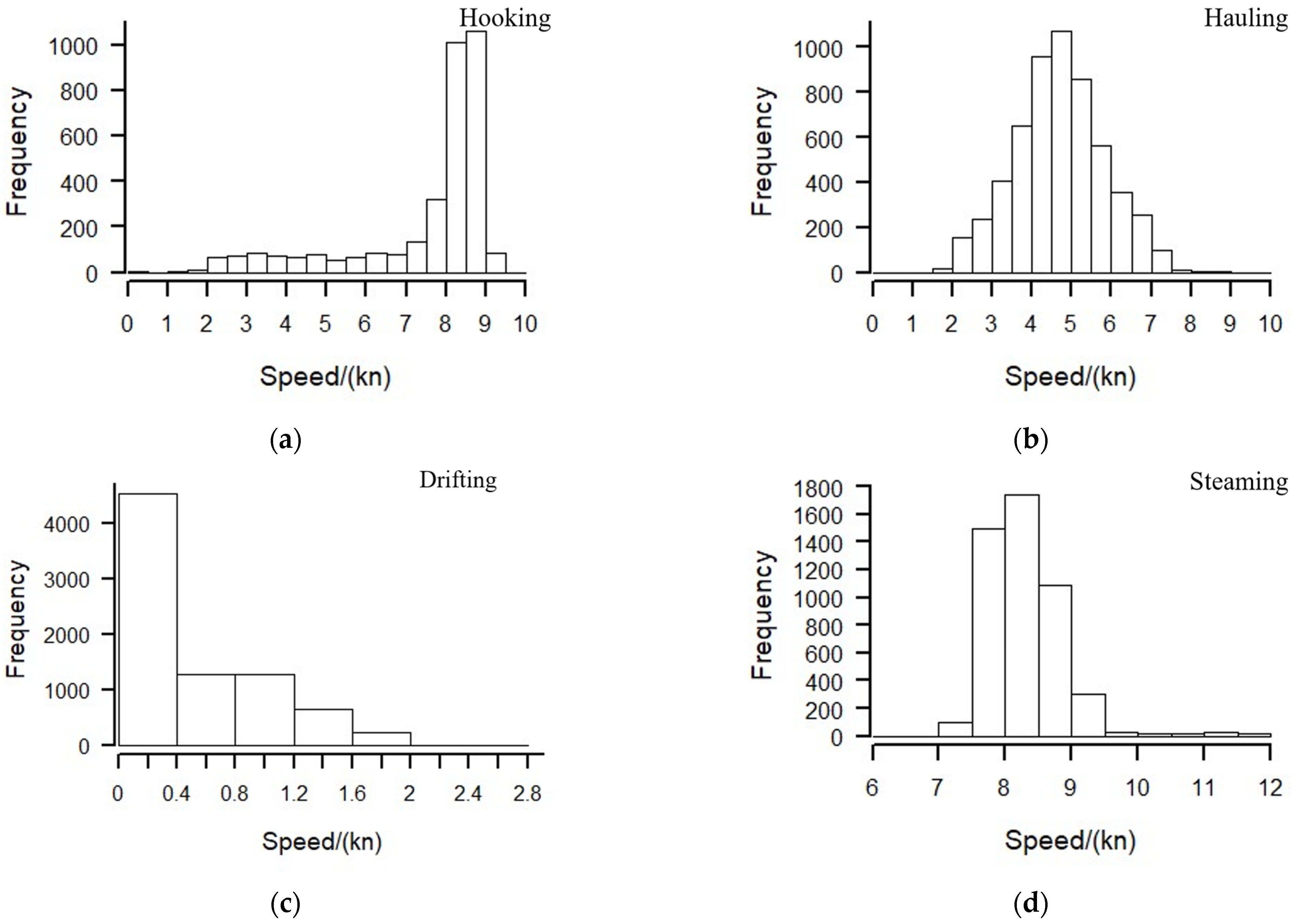
After manual status identification, the AIS data were categorised into hooking, hauling, drifting and steaming status, and frequency distribution statistics of the speed and course data of longliners under each status were performed to analyse the distribution and differences of the speed and course of longliners under each status. According to the diagram of the speed distribution of tuna longliners (Figure 2), the speed distribution of tuna longliners is unimodal in the four statuses. The speed distribution of tuna longliners in the hooking status ranged from 0 to 10 knots, with 76.18% of the speed distribution between 7 and 9 knots and the maximum frequency occurring between 8.5 and 9 knots. The speed distribution of tuna longliners in the hauling status was between 0 and 9 knots with a normal-like distribution, and the maximum speed occurred at 4.5 to 5 knots. In the drifting status, the distribution of the speed of tuna longliners ranged from 0 to 3 knots, with the maximum frequency occurring between 0 and 0.4 knots. In the steaming status, the distribution of the speeds of the tuna longliners ranged from 7 to 10 knots, and 91.39% of the speeds were distributed between 7.5 and 9 knots, with the maximum frequency occurring between 8 and 8.5 knots. The speeds of tuna longliners in the hauling and drifting status were lower than those in the hooking and steaming status.

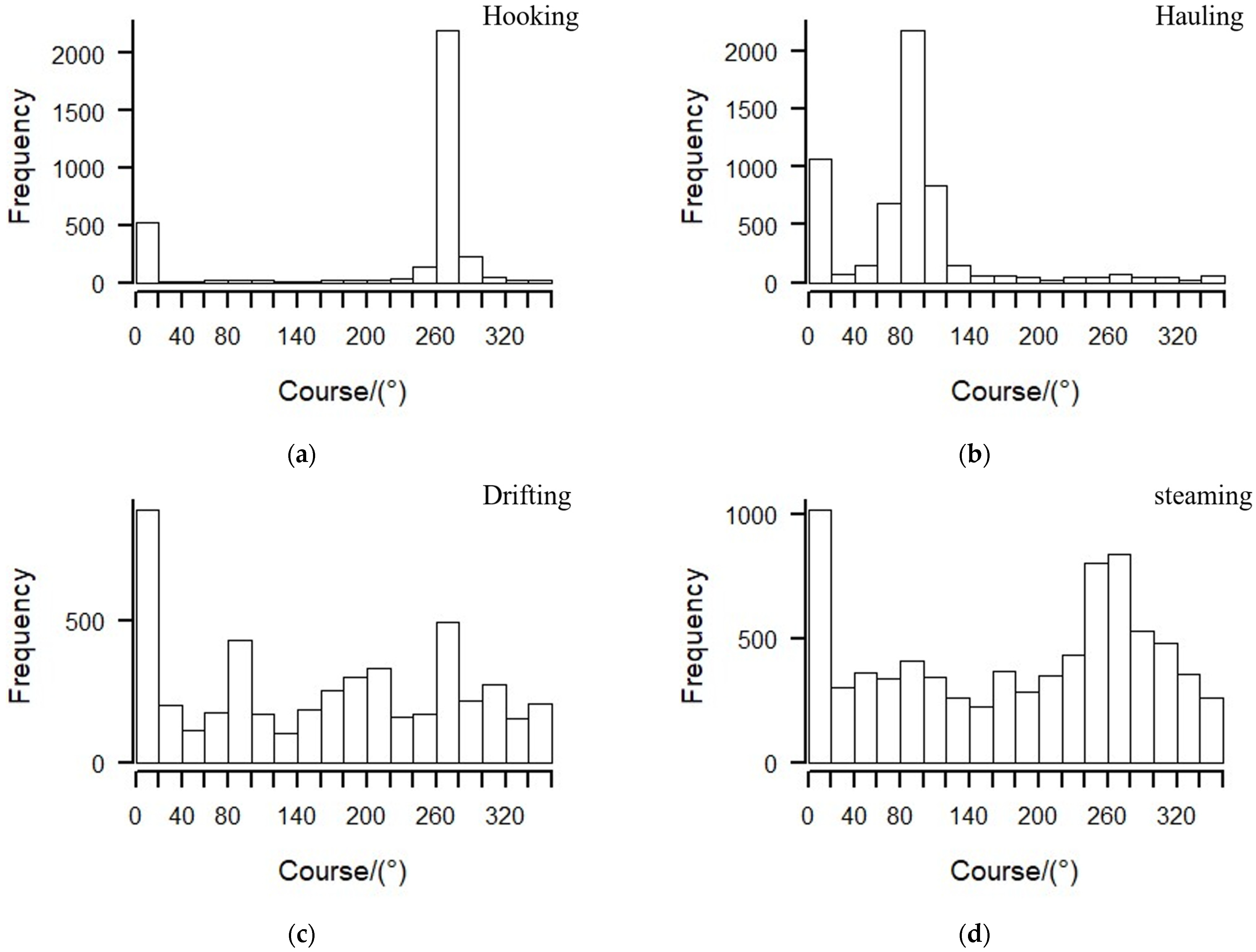
As can be seen from the course distribution diagram for tuna longliners (Figure 3), the course of tuna longliners in the hooking and hauling status has an approximately unimodal distribution, the course in the steaming status has an approximately bimodal distribution, and the course distribution characteristic of the drifting status is not significant. In the hooking status, 92.86% of the tuna longliners were distributed in the heading range of 0°~10° and 240°~300°, of which the peak heading was in the range of 260°~270°. In the hauling status, 89.60% of the tuna longliners had a course distribution between 0° and 10° and 60° and 120°, with the maximum course distribution between 80° and 90°. The course distribution of tuna longliners in the hooking and hauling status shows that the tuna longliners in the two statuses move in opposite directions, and this distribution characteristic is consistent with the actual operating characteristics of the vessels. In the drifting status, the distribution of the longliner course was more scattered, with a certain percentage of data randomly present throughout the 0° to 360° interval. Under the steaming status, the course peaks appeared at 60°~100° and 240°~280°, respectively, and based on the course distribution characteristics of tuna longliners under the steaming status, it can be seen that there is also a round trip phenomenon of tuna longliners under this status.

3.2. Threshold Screening Method

Based on the distribution characteristics of the speed and course of tuna longliners, the speed and course thresholds are set for screening the status of fishing vessels. The speed of a tuna longliner in drifting status is much lower than that of other statuses, so based on the distribution interval of the speed of a tuna longliner in drifting status, the data with a speed in the range of 0~2 knots are screened as drifting status. There are overlapping intervals in the distribution of speeds in the hooking, hauling and steaming status of tuna longliners, but the speeds in the hooking and hauling status are all lower than 9 knots, so 2~9 knots is used as the speed threshold for the operating status of tuna longliners. Since there is an overlapping interval of 8~9 knots in the distribution of speeds in the hooking and steaming status of tuna longliners, this study further filters the hooking and steaming status of tuna longliners by setting the course threshold. The first peak of the steaming status of tuna longliners occurs near 100°, while the peak of the hooking status occurs near 260°, so a course threshold of 240°~280° is set to exclude the steaming status of fishing vessels with speeds within 8~9 knots.

Based on the speed and course thresholds set above, the AIS data from tuna longliners were randomly selected for status identification, resulting in a total of 22,781 records. The identification results of the threshold screening method are presented in

Table 1. Threshold screening method classification results.

	Actual	Fishing Status	Non-Fishing Status
Estimated
Fishing status		8498	1727
Non-fishing status		508	11,540

. The number of non-fishing status records is 12,408, of which 11,540 are correctly identified and 508 are identified as fishing status, and the identification accuracy rate of non-fishing status is 93%. The number of fishing status records is 9006, of which 8498 are correctly identified and 1727 are identified as fishing status, and the identification accuracy of fishing status is 94.3%. The threshold screening method identified more non-fishing statuses than fishing statuses with an overall method identification accuracy of 89.9%.

3.3. BP Neural Network Classification Models

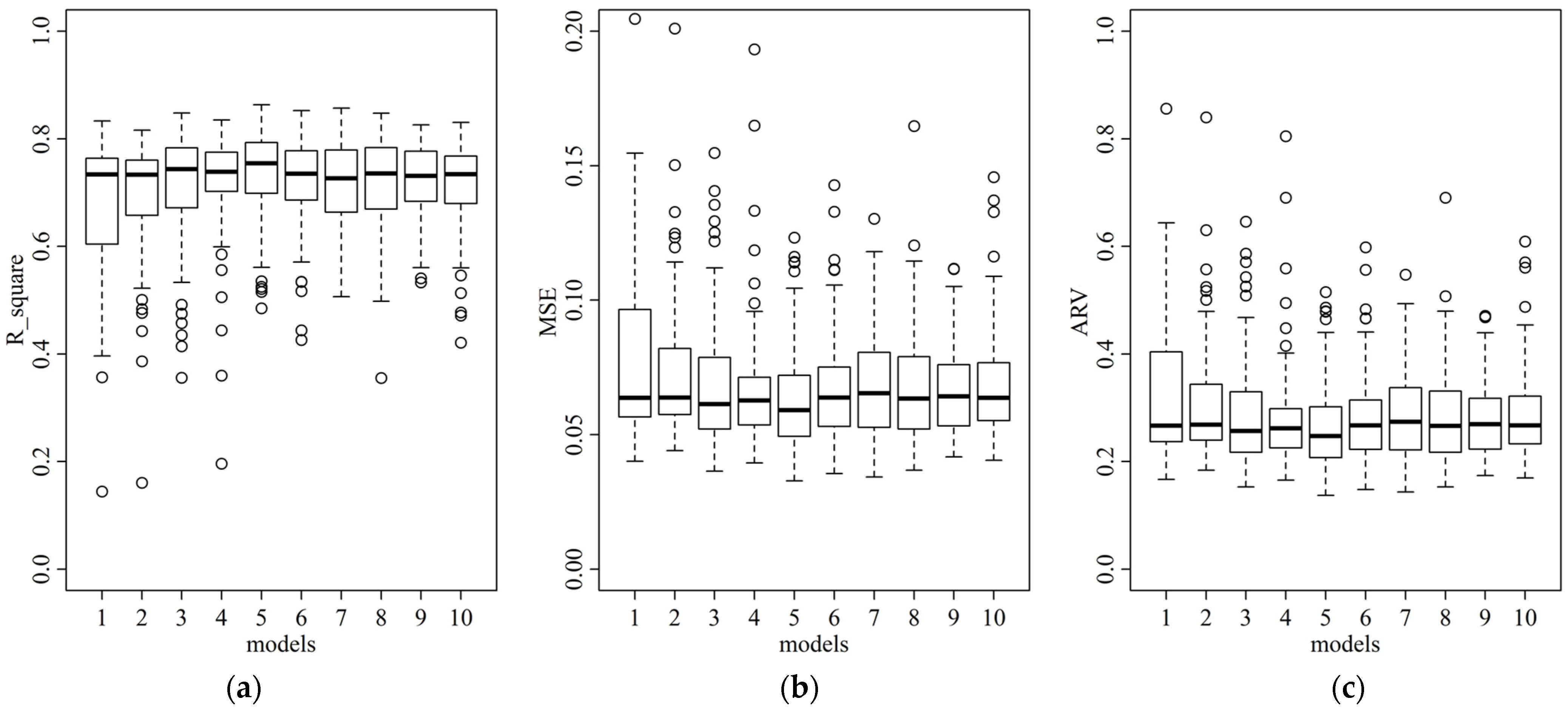
The number of input layers of the BP neural network constructed in the study is seven, the number of output layers is two, and the number of hidden layers of the neural network calculated based on the empirical formula ranges from three to thirteen, with a total of ten neural network models. The stability of each model was evaluated by multiple cross-validation. In each cycle, the data were randomly divided into training and test samples in the proportion of 70% and 30%, and after model training, the test samples were used to calculate the model accuracy indices. Based on the distribution of R², MSE and ARV values of 10 models obtained from 100 cycles, the optimal model is selected by combining the size and trend of the three indicators. The distribution of model accuracy shows that (Figure 4a) R² increases and then decreases with the number of hidden layer nodes, and the R² of model 5 is the largest; MSE fluctuates with the number of hidden layer nodes, and the MSE of model 5 is the smallest (Figure 4b); and the ARV shows a trend of decreasing and then increasing with the number of hidden layer nodes, and the ARV of model 5 is the lowest (Figure 4c). In addition to the fact that the three metrics, R², MSE and CRV, outperform the other models, we find that the box plot outliers for the three metrics deviate from model 5 less than the other models. In summary, the stability of model 5 is better, i.e., the neural network with hidden layer 7 is the optimal model.

The optimal model is selected for status identification for the training and validation sets, respectively. There are 14,334 training data, including 5840 fishing status records and 8494 non-fishing status records (

Table 2. Confusion table of training dataset for BP neural networks.

	Actual	Fishing Status	Non-Fishing Status
Estimated
Fishing status		5486	498
Non-fishing status		354	7996

). Among them, 5486 fishing status records and 7996 non-fishing status records are correctly identified (Table 2). The status discrimination accuracy of the model on the validation data set is 94.05%, the precision is 93.94%, the sensitivity is 91.68%, the specificity is 94.14% and the kappa coefficient is 0.51.

There are 6834 testing data, including 2799 fishing status records and 4035 non-fishing status records (

Table 3. Confusion table of testing dataset for BP neural networks.

	Actual	Fishing Status	Non-Fishing Status
Estimated
Fishing status		2586	121
Non-fishing status		213	3914

). Among them, 2586 fishing status records and 3914 non-fishing status records are correctly identified (Table 3). The status discrimination accuracy of the model on the validation data set is 95.11%, the precision is 92.39%, the sensitivity is 95.53%, the specificity is 97% and the kappa coefficient is 0.51.

3.4. SVM Models

We employed C-support vector classification (C-SVC) to build the classification model, with the radial basis function (RBF) kernel function chosen. RBF kernel function exhibits lower numerical computational complexity when compared to other kernel functions [19]. The optimal penalty factor c, and parameter g, were obtained through the cross-validation method. Values of c and g ranged from 2⁻¹⁰ to 2¹⁰, with an interval of 2^0.2. The optimal parameters of the SVM model were obtained using the cross-validation method. Results indicate that the parameters c and g are optimal when set to 1 and 4, respectively, based on cross-validation outcomes.

The optimal model is selected for status identification for the training and validation sets, respectively. There are 15,945 training data, including 6288 fishing status records and 9657 non-fishing status records (

Table 4. Confusion table of training dataset for SVM.

	Actual	Fishing Status	Non-Fishing Status
Estimated
Fishing status		6025	468
Non-fishing status		263	9189

). Among them, 6025 fishing status records and 9189 non-fishing status records are correctly identified (Table 4). The status discrimination accuracy of the model on the validation data set is 95.41%, the precision is 95.81%, the sensitivity is 92.79%, the specificity is 95.15% and the kappa coefficient is 0.52.

There are 6835 testing data, including 2718 fishing state records and 4117 non-fishing status records (

Table 5. Confusion table of testing dataset for SVM.

	Actual	Fishing Status	Non-Fishing Status
Estimated
Fishing status		2602	175
Non-fishing status		116	3942

). Among them, 2602 fishing status records and 3942 non-fishing status records are correctly identified (Table 5). The status discrimination accuracy of the model on the validation data set is 95.74%, the precision is 95.73%, the sensitivity is 93.69%, the specificity is 95.74% and the kappa coefficient is 0.52.

3.5. Fishing Effort Statistics

Based on the SVM classification model identification results, we counted the fishing days and fishing hours of these five tuna longliners for the period from 2021 to 2022. The average number of trips made by the five fishing vessels in 2021 was 16, with an average of 11 days per trip; the average number of trips made in 2022 was 18, with an average of 12 days per trip. And their frequency distributions were counted by month (Figure 5). The monthly distribution of the number of fishing days of the fishing vessels was more even, with the number of operating days in June being higher than the rest of the months. The peak of the months of fishing hours of fishing vessels was also in June, but there was a difference in the monthly distribution of fishing days, and the fishing hours were mainly concentrated in the second half of the year.

3.6. Spatial Distribution of Fishing Effort

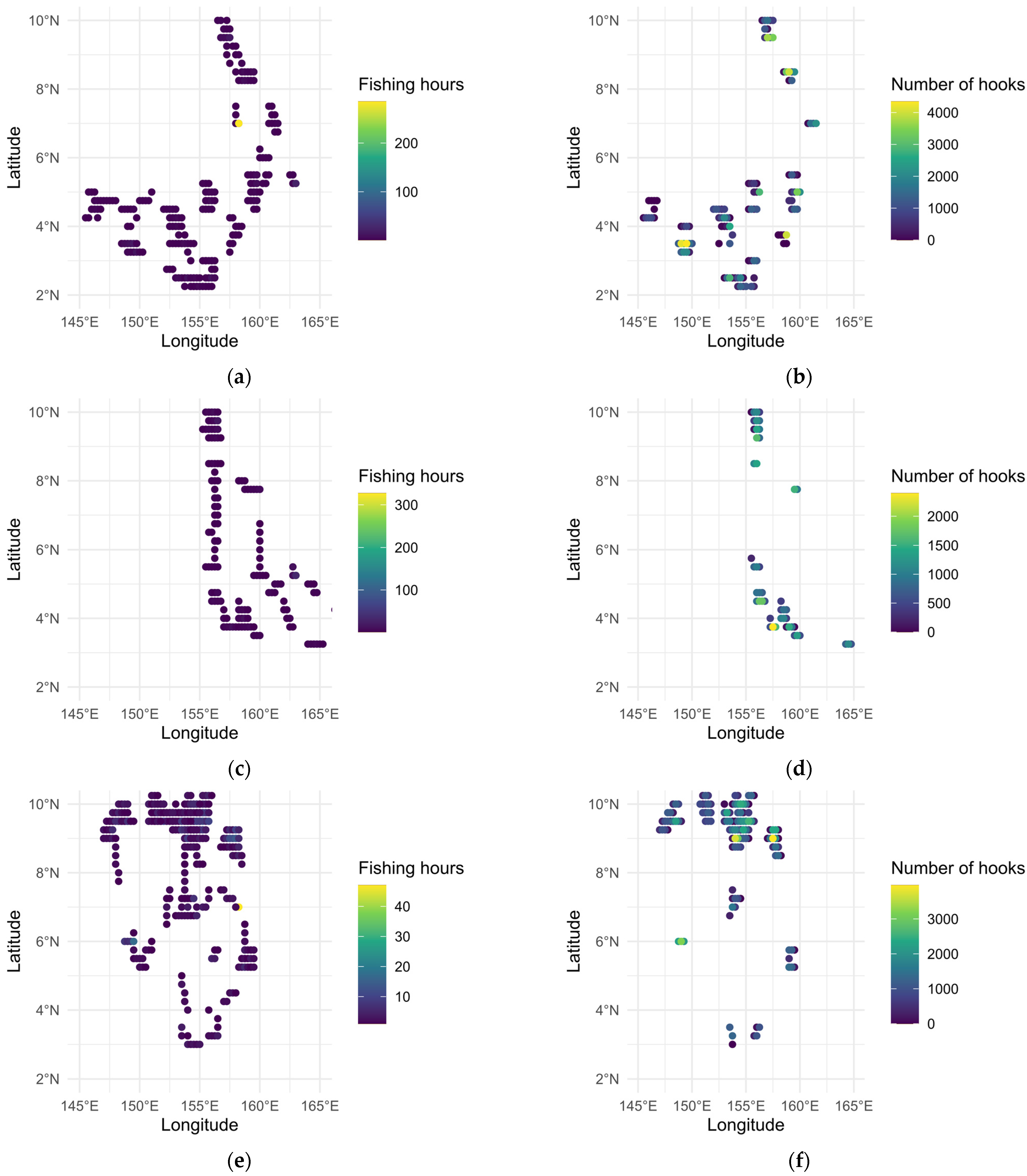
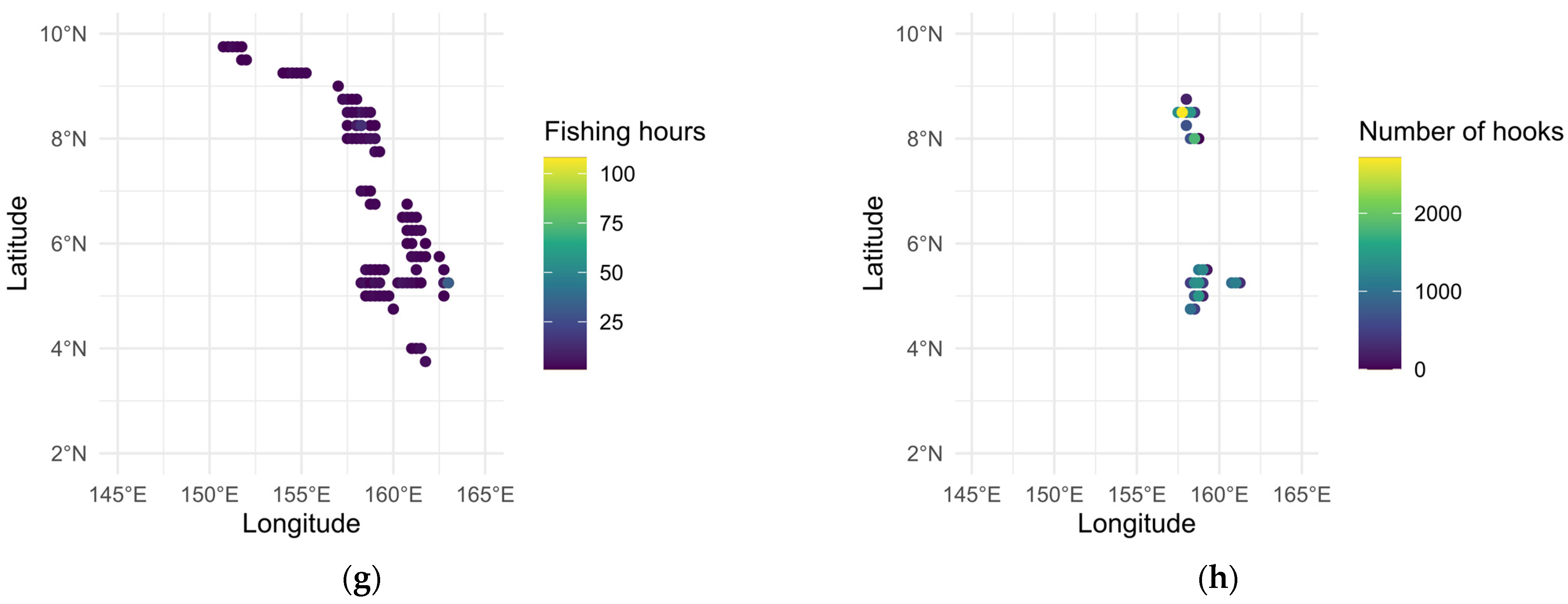
After assessing the accuracy of identification methods, we have selected the support vector machine (SVM) model as the most appropriate for determining the status of the tuna longliner’s Automatic Identification System (AIS) data. We have quantified the duration of VESSEL A’s fishing activity through the cumulative time elapsed between its operational status points. The fishing effort’s spatial distribution was plotted by model identification results and fishing logbook records with consideration to the quarter (Q1 for January, Q2 for June, Q3 for July to September, and Q4 for November) (Figure 6). There were discernible disparities in the spatial allocation of fishing activity across quarters. In Q1, the intensive area of operation of VESSEL A was located at 145°~160° E, 2°~5° N. In Q2, the intensive area of operation of VESSEL A was located at 155°~160° E, 3°~6° N. In Q3, the intensive area of operation of VESSEL A was located at 145°~160° E, 8°~10° N. In Q4, VESSEL A had two intensive operation areas located at 155°~160° E, 4°~6° N and 8°~9° N, respectively. The spatial distribution of VESSEL A’s operations in 2021 exhibited a trend towards the north of the centre of gravity in the first half of the year and towards the south in the second half of the year. In addition, there is a significant spatial similarity between cumulative operating time and hook-quantified fishing effort, although the distribution of cumulative operating time was more widespread.

3.7. Spatial Correlation Analysis

VESSEL A operated during the months of January, June, July, August, September, October and November in 2021. Cumulative operating time data and the number of hooks data were combined by month to compute the two corresponding fishing effort values for each grid, which were subjected to the Pearson correlation test.

Table 6. Monthly spatial correlation analysis of two fishing effort estimates for VESSEL A.

Month	January	June	July	August	September	October	November
Pearson’s correlation coefficient	0.88	0.98	0.88	0.79	0.84	0.99	0.99

presents the test results. The correlation coefficients between the two different types of fishing effort were greater than 0.79 for each month. Moreover, for the months of June, October and November, the correlation coefficients were greater than 0.98. This suggests that there were no significant differences in the spatial and temporal distribution of the two types of effort.

4. Discussion

4.1. The Reliability of This Study Are High

A longline fishing set typically involves a fast hook deployment operation in the morning and a slower retrieval operation (including processing of the catch) in the afternoon (till midnight or dawn) [28]. Navigational characteristics such as time, speed and course are also different between different statuses of longliners, and all of these data are available in the fishing vessel monitoring data. Chang et al. [28] were the first to define a fishing day for longliners by setting the time-of-day period and speed thresholds for vessel operations. While a simple speed ruler was easy to apply as a behaviour classification approach to separate the fishing and non-fishing status of tuna longliners [29], there is an overlap in the distribution of speeds between the different statuses of longline fishing vessels [28], leading to an overestimation of the fishing effort of the vessels [19]. Furthermore, the vessel position monitoring data used by early scholars were obtained from VMS. However, due to the reporting interval of this data being more than 4 h per day, the course data provided insufficient information to determine the behaviour of the fishing vessels [30]. With the advent of the AIS, initially implemented for ship-to-ship collision avoidance, the temporal resolution of monitoring has been further refined from hours to minutes or seconds [31]. AIS enables the extraction of additional data on the navigation characteristics of longliners. At present, scholars have mined the information of the time, range distance, speed and speed difference, heading and heading difference in fishing vessels in AIS data for longline fishing vessels‘ status identification [19,20,21], trajectory reconstruction [32,33,34], and other research. In addition, the operating vessels in the study area of this paper are all small tuna longliners, so there is no need to consider differences over time or between vessels.

4.2. SVM Is the Optimal Method

Fisheries research using vessel monitoring data has two phases: identification of the fishing status and calculation of fishery-related metrics [34]. High accuracy in identifying the behaviour of fishing vessels is a critical step in estimating fishing vessel activity and effort [35]. At present, methods for identifying the status of fishing vessels can be broadly divided into two categories: threshold screening methods and the construction of classification models. Various methods have been used to estimate fishing vessel behaviour using AIS data, including setting speed and course thresholds [17], constructing neural network models [19], constructing SVM models [18], etc. In order to investigate the relative optimal methods for the status identification of tuna longliners, we adopt the three methods mentioned above to investigate the status identification of tuna longliners, respectively, and calculate the accuracy rate and kappa coefficient as a measure of the relative optimal methods.

The threshold screening method achieved a recognition accuracy of 89.9%, while the BP neural network and SVM models achieved 95.11% and 95.74% accuracy, respectively. The kappa coefficient for the BP neural network and SVM models were 0.51 and 0.52, respectively. Both classification models constructed for the training and validation datasets achieved over 90% for all classification metrics, surpassing the results of the threshold screening method. The findings align with those of previous research [17,18,19]. The frequency distribution plot of the speed and course distribution of longline fishing vessels shows overlapping intervals for the speed and course of fishing vessels in different statuses. Therefore, setting a fixed threshold interval for speed and heading may result in a misjudgement of the status of the fishing vessel. The method of identification for constructing a classification model is more appropriate for this case due to the non-linear relationship between the data on fishing vessel speed and heading characteristics and the status of the fishing vessel [36]. The BP neural network model and SVM model are widely used in fishery scientific research, such as CPUE standardisation [37,38] and fishery forecasting [39], due to their autonomous learning ability, strong generalisation, and fault tolerance. The SVM model we constructed is more accurate than the BP neural network classification model. This demonstrates that the SVM method outperforms the BP neural network classification model in identifying the state of longliners. Therefore, we chose to launch a subsequent fishing effort estimation study based on the constructed SVM classification model.

4.3. AIS Data Are More Suitable for the Fishing Effort Spatial Distribution Estimation

For longline fishery, nominal fishing effort is almost always represented as the number of hooks deployed [40]. However, the AIS data do not provide information for estimating the number of hooks used [28]. The tuna longliner performs a single operation set per day, using a fixed number of hooks in each set [41]. Therefore, previous studies have mainly used fishing days [28] or cumulative operating time [22] to represent fishing effort. In this study, we chose to measure the fishing effort of longliners in terms of cumulative operating time, and at the same time calculated the fishing effort in terms of the number of hooks based on fishing logbook data and plotted the spatial distribution of fishing effort in terms of seasons (Figure 5).

The distribution maps showed that the spatial distribution of fishing effort and duration of operation are similar, but the latter has a greater number of fishing areas. There are three potential reasons for variations in the distribution of two units of effort data: (a) Different temporal resolutions: Logbook data only records the location of the deployment, providing low coverage fishing effort data [20]. In contrast, AIS data reports the dynamics of the voyage throughout the day at a certain reporting frequency. (b) Variations in the accuracy of latitude and longitude data: Fishers do not record fishing locations simultaneously with fishing operations, making the recorded location potentially different from the actual fishing location [42]. (c) Error identification in SVM identification models: There are 6.3% of VMS-based fishing locations that were not found in the logbook-based data.

Furthermore, the spatial distribution of fishing effort estimated from cumulative operating time based on AIS data is more refined than the number of hooks. In addition, we performed spatial and temporal fusion statistics of the two units of fishing effort data at a spatial resolution of 0.25° × 0.25° latitude and longitude and analysed them for spatial correlation. The results of the correlation analysis showed that the correlation coefficients between the two types of effort were greater than 0.79 on all fishing months, indicating that there was no significant difference in the spatial and temporal distribution between the two types of effort.

5. Conclusions

In summary, based on the AIS data of tuna longliners from 2020 to 2021, we adopted the speed and sailing threshold screening method, and the construction of the BP neural network and SVM classification model, respectively, to carry out the status identification research on longliners. The identification accuracy of the SVM classification model is 95.74% with a kappa coefficient of 0.52, and the results of the training set and test set of this model are better than the other two methods. Therefore, the constructed optimal SVM classification model was chosen to identify the status of VESSEL A, and the fishing effort was quantified by calculating the cumulative operating time in the fishing area based on the identification results. Fishing effort in terms of the number of hooks was also calculated based on fishing logbook data, and spatial distribution maps and spatial correlation analyses were prepared for each of the two types of fishing effort. The results of this study showed a finer spatial distribution in fishing effort mapped through the AIS data and a significant correlation between the results of the fishing logbook. The SVM model can be used to identify the status and estimate the fishing effort of longliners. In addition, there are many factors affecting the navigational differences between the states of longliners, such as wind and current variations, etc., and the focus of the subsequent research remains on mining more feature variables and constructing more appropriate status identification models.

References

1. Russo, T.; Carpentieri, P.; Fiorentino, F.; Arneri, E.; Scardi, M.; Cioffi, A.; Cataudella, S. Modeling landings profiles of fishing vessels: An application of Self-Organizing Maps to VMS and logbook data. Fish. Res. 2016, 181, 34–47. [Google Scholar] [CrossRef]
2. Fonseca, T.; Campos, A.; Afonso-Dias, M.; Fonseca, P.; Pereira, J. Trawling for cephalopods off the Portuguese caost-Fleet dynamics and landing composition. Fish. Res. 2008, 92, 180–188. [Google Scholar] [CrossRef]
3. Okamura, H.; Morita, S.H.; Funamoto, T.; Ichinokawa, M.; Eguchi, S. Target-based catch-per-unit-effort standardization in multispecies fisheries. Can. J. Fish. Aquat. Sci. 2018, 75, 452–463. [Google Scholar] [CrossRef]
4. Yadav, V.K.; Jahageerdar, S.; Adinarayana, J. Use of different modeling approach for sensitivity analysis in predicting the Catch per Unit Effort (CPUE) of fish. Indian J. Geo-Mar. Sci. 2020, 49, 1729–1741. [Google Scholar]
5. Mullowney, D.R.; Dawe, E.G. Development of performance indices for the Newfoundland and Labrador snow crab (Chionoecetes opilio) fishery using data from a vessel monitoring system. Fish. Res. 2009, 100, 248–254. [Google Scholar] [CrossRef]
6. Walters, C. Folly and fantasy in the analysis of spatial catch rate data. Can. J. Fish. Aquat. Sci. 2003, 60, 1433–1436. [Google Scholar] [CrossRef]
7. Janette, L.; South, A.B.; Simon, J. Developing reliable, repeatable, and accessible methods to provide high-resolution estimates of fishing-effort distributions from vessel monitoring system (VMS) data. ICES J. Mar. Sci. 2010, 67, 1260–1271. [Google Scholar]
8. Bertrand, S.; Burgos, J.M.; Gerlotto, F.; Atiquipa, J. Lévy trajectories of Peruvian purse-seiners as an indicator of the spatial distribution of anchovy (Engraulis ringens). ICES J. Mar. Sci. 2005, 62, 477–482. [Google Scholar] [CrossRef]
9. Natale, F.; Gibin, M.; Alessandrini, A.; Vespe, M.; Paulrud, A. Mapping Fishing Effort through AIS Data. PLoS ONE 2015, 10, e0130746. [Google Scholar] [CrossRef]
10. Murawski, S.A.; Wigley, S.E.; Fogarty, M.J.; Rago, P.J.; Mountain, D.G. Effort distribution and catch patterns adjacent to temperate MPAs. ICES J. Mar. Sci. 2005, 62, 1150–1167. [Google Scholar] [CrossRef]
11. Gerritsen, H.; Lordan, C. Integrating vessel monitoring systems (VMS) data with daily catch data from logbooks to explore the spatial distribution of catch and effort at high resolution. ICES J. Mar. Sci. 2011, 68, 245–252. [Google Scholar] [CrossRef]
12. Bez, N.; Walker, E.; Gaertner, D.; Rivoirard, J.; Gaspar, P. Fishing activity of tuna purse seiners estimated from vessel monitoring system (VMS) data. Can. J. Fish. Aquat. Sci. 2011, 68, 1998–2010. [Google Scholar] [CrossRef]
13. Walker, E.; Gaertner, D.; Gaspar, P.; Bez, N. Fishing activity of tuna purse estimated from VMS data and validated by observers’ data. Collect. Vol. Sci. Pap. 2010, 65, 2376–2391. [Google Scholar]
14. Murray, L.G.; Hinz, H.; Hold, N.; Kaiser, M.J. The effectiveness of using CPUE data derived from Vessel Monitoring Systems and fisheries logbooks to estimate scallop biomass. ICES J. Mar. Sci. 2013, 70, 1330–1340. [Google Scholar] [CrossRef]
15. James, M.; Mendo, T.; Jones, E.; Orr, K.; McKnight, A.; Thompson, J. AIS data to inform small scale fisheries management and marine spatial planning. Mar. Policy 2018, 91, 113–121. [Google Scholar] [CrossRef]
16. Kroodsma, D.; Mayorga, J.; Hochberg, T.; Miller, N.; Boerder, K.; Ferretti, F.; Wilson, A.; Bergman, B.; White, T.; Block, B.; et al. Tracking the Global Footprint of Fisheries. Science 2018, 359, 904–908. [Google Scholar] [CrossRef]
17. Yang, S.L.; Zhang, S.M.; Yuan, Z.H.; Dai, Y.; Zhang, H.; Zhang, B.B.; Fan, W. Calculating the fishing intensity of offshore longline fleets on fishing grounds based on their fishing characteristics. J. Fish. Sci. China 2020, 27, 307–314. [Google Scholar]
18. Yang, S.L.; Zhang, S.M.; Zhou, W.F.; Cui, X.S.; Zhang, B.B.; Fan, W. Calculating the fishing effort of longline fishing vessel in the western and central pacific ocean using AIS. Trans. Chin. Soc. Agric. Eng. 2020, 36, 198–203. [Google Scholar]
19. Nieblas, A.; Barde, J.; Louys, J.; Assan, C.; Imzilen, T.; Dalleau, C.; Gerry, C.; Chassot, E. Global Atlas of AIS-Based Fishing Activity—Challenges and Opportunities; FAO: Rome, Italy, 2019. [Google Scholar]
20. Iriondo, A.; Santiago, J.; Murua, H.; Granado, I.; Taconet, M.; Kroodsma, D.; Miller, N.; Fernandes, J. FAO Area 67—AIS-Based Fishing Activity in the Northeast Pacific; FAO: Rome, Italy, 2019. [Google Scholar]
21. Yuan, Z.H.; Yang, D.H.; Fan, W.; Zhang, S.M. On fishing grounds distribution of tuna longline based on satellite automatic identification system in the Western and Central Pacific. Mar. Fish. 2018, 40, 649–659. [Google Scholar]
22. Bordalo, M.P.; Figueiredo, I. Extraction and classification of longline fishing trips from vessel monitoring systems data with sequential recording gaps. Int. Arch. Photogramm. Remote Sens. Spat. Inf. Sci. 2007, 34, 1–7. [Google Scholar]
23. Song, L.M.; Lv, K.K.; Yang, J.L.; Hu, Z.X. Otolith morphology of bigeye tuna in Marshall Islands waters. J. Shanghai Ocean Univ. 2012, 21, 884–891. [Google Scholar]
24. Cheng, X.; Zhang, F.; Chen, X.J.; Wang, J.T. Application of Artificial Intelligence in the Study of Fishing Vessel Behavior. Fishes 2023, 8, 516. [Google Scholar] [CrossRef]
25. Ciaburro, G.; Venkateswaran, B. Neural Networks with R: Smart Models Using CNN, RNN, Deep Learning, and Artificial Intelligence Principles; Packt Publishing Ltd.: Birmingham, UK, 2017. [Google Scholar]
26. Wang, P.; Wang, P.; En, F. Neural Network Optimization Method and Its Application in Information Processing. Math. Probl. Eng. 2021, 2, 10. [Google Scholar] [CrossRef]
27. Li, Z.; Ye, Z.; Wan, R.; Zhang, C. Model selection between traditional and popular methods for standardizing catch rates of target species a case study of Japanese Spanish mackerel in the gillnet fishery. Fish. Res. 2015, 161, 312–319. [Google Scholar] [CrossRef]
28. Chang, S.K.; Yuan, T.L. Deriving high-resolution spatiotemporal fishing effort of large-scale longline fishery from vessel monitoring system (VMS) data and validated by observer data. Can. J. Fish. Aquat. Sci. 2014, 71, 1363–1370. [Google Scholar] [CrossRef]
29. Marza, I.M. VMS Data Analyses and Modeling for the Monitoring and Surveillance of Indonesian Fisheries. Ph.D. Thesis, Computer Vision and Pattern Recognition. Ecole Nationale Supérieure Mines-Télécom Atlantique, Nantes, France, 2017. [Google Scholar]
30. Witt, M.J.; Godley, B.J. A step towards seascape scale conservation: Using vessel monitoring systems (VMS) to map fishing activity. PLoS ONE 2017, 2, e1111. [Google Scholar] [CrossRef] [PubMed]
31. Robards, M.D.; Silber, G.K.; Adams, J.D.; Arroyo, J.; Lorenzini, D.; Schwehr, K.; Amos, J. Conservation science and policy applications of the marine vessel Automatic Identification System (AIS)—A review. Bull. Mar. Sci. 2016, 92, 75–103. [Google Scholar] [CrossRef]
32. Guo, S.Q.; Mou, J.M.; Chen, L.Y.; Chen, P.F. Improved Kinematic Interpolation for AIS Trajectory Reconstruction. Ocean Eng. 2021, 234, 109256. [Google Scholar] [CrossRef]
33. Zhang, L.Y.; Meng, Q.; Xiao, Z.; Fu, X.J. A novel ship trajectory reconstruction approach using AIS data. Ocean Eng. 2018, 159, 165–174. [Google Scholar] [CrossRef]
34. Huang, H.G.; Hong, F.; Liu, J.; Liu, C.; Feng, Y.; Guo, Z.W. FVID: Fishing Vessel Type Identification Based on VMS Trajectories. J. Ocean Univ. China 2019, 18, 403–412. [Google Scholar] [CrossRef]
35. Yang, S.L.; Shi, H.M.; Fan, W.; Zhang, H.; Fei, Y.J.; Zhang, H. Spatial distribution of squid fishing vessel operations in the southwest Atlantic Ocean and its relationship with environmental factors. J. Fish. Sci. China 2022, 29, 365–376. [Google Scholar]
36. Shono, H. Application of support vector regression to CPUE analysis for southern bluefin tuna Thunnus maccoyii and its comparison with conventional methods. Fish Sci. 2014, 80, 879–886. [Google Scholar] [CrossRef]
37. Mao, J.M.; Chen, X.J.; Jing, Y. Forecasting fishing ground of Thunnus alalunga based on BP neural network in the South Pacific Ocean. Acta Oceanol. Sin. 2016, 38, 34–43. [Google Scholar]
38. Yang, S.L.; Zhang, Y.; Zhang, H.; Fan, W. Comparison and analysis of different model algorithms for CPUE standardization in fishery. Trans. Chin. Soc. Agric. Eng. 2015, 31, 259–264. [Google Scholar]
39. Yuan, H.C.; Gu, Y.T.; Wang, J.T.; Chen, Y.; Chen, X.J. Study on the Medium and Long Term of Fishery Forecasting Based on Neural Network. In Proceedings of the Artificial Intelligence and Computational Intelligence: 4th International Conference, AICI 2012, Chengdu, China, 26–28 October 2012; Proceedings 4. Springer: Berlin/Heidelberg, Germany, 2012; pp. 626–633. [Google Scholar]
40. Campbell, R.A. CPUE standardisation and the construction of indices of stock abundance in a spatially varying fishery using general linear models. Fish. Res. 2014, 70, 209–227. [Google Scholar] [CrossRef]
41. Ward, P.; Hindmarsh, S. An overview of historical changes in the fishing gear and practices of pelagic longliners, with particular reference to Japan’s Pacific fleet. Rev. Fish Biol. Fish. 2007, 17, 501–516. [Google Scholar] [CrossRef]
42. Gunawardane, N.; Ariyarathna, M.; Amarasinghe, U.; de Croos, D. Validating the fishing locations reported in the logbooks using the positional data of vessel monitoring systems in the multi-day fishery of Sri Lanka. Sri Lanka J. Aquat. Sci. 2023, 28, 11–28. [Google Scholar] [CrossRef]
Figure 1. AIS data cleaning flowchart.
Fishes 09 00066 g001
Figure 2. Speed distribution of tuna longliners under different statuses: (a) hooking; (b) hauling; (c) drifting; and (d) steaming.
Fishes 09 00066 g002
Figure 3. Course distribution of tuna longliners under different statuses: (a) hooking; (b) hauling; (c) drifting; and (d) steaming.
Fishes 09 00066 g003
Figure 4. Distribution of R2, MSE and ARV values for all neural network models: (a) R2 value; (b) MSE value; and (c) ARV value. Discrete points in the graph indicate outliers.
Fishes 09 00066 g004
Figure 5. Monthly distribution of fishing effort by tuna longline fishing vessels: (a) fishing days; and (b) fishing hours.
Fishes 09 00066 g005
Figure 6. Spatial distribution of fishing effort of VESSEL A: (a) spatial distribution in terms of cumulative fishing hours in Q1; (b) spatial distribution in terms of number of hooks in Q1; (c) spatial distribution in terms of cumulative fishing hours in Q2; (d) spatial distribution in terms of number of hooks in Q2; (e) spatial distribution in terms of cumulative fishing hours in Q3; (f) spatial distribution in terms of number of hooks in Q3; (g) spatial distribution in terms of cumulative fishing hours in Q4; and (h) spatial distribution in terms of number of hooks in Q4.
Fishes 09 00066 g006aFishes 09 00066 g006b