Semi-Automated Inquiry of Fish Launch Angle and Speed for Hazard Analysis

Abstract

This study investigated the leap characteristics of rainbow trout (also known as steelhead) (Oncorhynchus mykiss) present in the Laurentian Great Lakes. To aid in the collection and annotation of leaps, a custom web application was developed and through the labeling of key markers, the launch speed, launch angle, and length of the fish were calculated. Data collection took place during migratory runs in the spring of 2022 and 2023 that resulted in 173 total leaps annotated with mean launch angles of 58.73 and 68.2 degrees, in 2022 and 2023, respectively. The mean launch speed normalized by body length was consistent across years at 8.6 body lengths per second. The integration of leaping data with computational fluid dynamics simulations revealed steelhead launch angle aligns closely with the water velocity direction as the velocity magnitude increases. Applications of this study include hazard analyses for unintended escapement and informed design of intelligent migratory barriers such as those to be developed at FishPass, an instream research facility under design for the Boardman (Ottaway) River in Traverse City, MI, USA.

1. Introduction

Aquatic invasive species significantly affect enterprises such as fisheries, agriculture, and international trade [1]. In the Laurentian Great Lakes basin (hereafter referred to as the Great Lakes), invasive sea lamprey (Petromyzon marinus) present a significant threat to its fisheries. In the early 1900s, sea lamprey entered the basin and due to their devastating feeding habits, contributed to the near-complete extirpation of lake trout (Salvelinus namaycush) and lake whitefish (Coregonus clupeaformis) [2,3]. Among the available options to protect these fisheries from invaders, physical barriers are one of the most cost-effective and reliable solutions, but they still involve trade-offs [4]. While barriers prevent the entry of harmful and invasive species into spawning habitats and, in the Great Lakes, allow the use of pesticidal treatment to kill sea lamprey larvae in tributaries [5], barriers also limit the movement of native and other desirable fish. Typical sea lamprey barriers, for example, have a 45 cm vertical gap between the barrier crest and downstream water levels [6]. Fish with strong swimming and leaping skills, such as Pacific salmonids, transferred to the Great Lakes, are generally able to pass upstream, but species native to the Great Lakes have limited tendency or abilities to leap over the barriers and consequently, have exhibited little success in overcoming these conventional barriers. Lake trout, cisco (Coregonus artedi), lake whitefish (Coregonus clupeaformis), walleye (Sander vitreus), suckers (Catostomus spp.), burbot (Lota lota), and lake sturgeon (Acipenser fulvescens) are among the native species that use tributaries as their primary spawning and nursery habitats and must deal with the effects of barriers [7,8]. Additionally, barriers such as hydroelectric dams damage hundreds of thousands of fish each year as fish come into contact with the dam’s turbines [9].

Human built fishways are intended to provide migrating fish with a means to bypass otherwise non-traversable barriers such as dams. Many fishways were designed using specifications meant for salmonids [10] and create hydraulic conditions that limit passage rates of fish with limited swimming or leaping abilities when compared to anadromous salmonids [11]. Even passage rates of salmonids through various fishway types can vary between 20–80% [12]. Subsequent lack of passage or delays in passage timing can have detrimental impacts on fishes during both downstream and upstream migrations [13,14,15,16,17]. Efforts around the world are underway to improve fishway designs for both salmonid and non-salmonid species [18,19]. However, with the exception of trap-and-sort operations, current fishway technologies are unable to deal with the difficulties of fish assemblages containing both native and invasive species, each with competing management goals concerning passage.

To address the drawbacks of conventional barriers and fishway designs, the Great Lakes resource managers are seeking solutions that keep invasive species under control while boosting river connectivity for native fishes [6]. Selective connectivity, where organism movement is selective in terms of taxa and potentially individuals based on restoration or conservation goals and objectives, presents a potential solution to the connectivity conundrum facing barrier decisions in fragmented systems [20]. Following the framework developed in the material recycling industry, selective passage solutions for a mixed assemblage of fish should emphasize both automation and attribute-based sorting processes which account for variability in phenological, morphological, behavioral, and physiological attributes of the assemblage [20,21]. A fundamental aspect of selective passage is that all passage opportunities are managed; thus, uncontrolled passage of both desirable and undesirable species must be minimized.

Unlike sea lamprey, which are undoubtably undesirable, the desirability of other species introduced to the Great Lakes depends upon a variety of ecological, economic, cultural, and social factors. While stocked Pacific salmonids, including chinook salmon (Oncorhynchus tshawytshca), coho salmon (Oncorhynchus kisutch), and ad fluvial rainbow trout (also known as steelhead) (Oncorhynchus mykiss), are highly valued sportfish, their access into previously inaccessible watersheds (i.e., like those above previously impassable barriers) can have both positive and negative intraspecific effects on resident brook trout (Salvelinus fontinalis) and brown trout (Salmo trutta) populations [22]. Thus, the management of Pacific salmonid passage at barriers or as a result of barrier removals is site specific. Pacific salmonids also present a unique challenge to selective fish passage solutions as their prolific leaping abilities make containment of uncontrolled passage in the predominately low gradient tributaries of the Great Lakes basin difficult. To evaluate the potential risk of unintended, volitional passage at new barriers or passage systems, the leaping abilities and behaviors of migrating Pacific salmonids in the Great Lakes must be quantified.

Of all introduced salmonids in the Great Lakes, steelhead have the greatest estimated swimming speed and, thus leaping height [23], and are the focus of this study. Powers and Osborn [24] estimate steelhead are capable of leaping in excess of 3 m high. Their leaping abilities are already accounted for in the design of pool and weir fishways which are the most prominent fishway type in the Great Lakes [25]. Steelhead also exhibit a panoply of life history and migratory patterns both in the Great Lakes and in its native range [26,27,28]. In the Great Lakes, steelhead migrate into tributaries to spawn between November and July at 0.5–18 °C, with peak spawning usually occurring between April and May at 6–8 °C [28].

The key parameters used to estimate fish passage via leaping over a barrier are launch speed and launch angle. When examining the maximum leap height of fish, launch speed is assumed to be equivalent to a fish’s maximum burst swim speed. While studies have quantified swimming performance, and hence maximum burst speed, of large, and presumably adult, steelhead [29,30], the possible range of maximum burst swim speed is large. Weaver [29] found the burst swimming speed of six individual adult steelhead (total length > 610 mm) ranged between 7–13.4 body lengths per seconds (BL/s). Katapodis and Gervais [30] collected swim speed versus time-to-fatigue data from 1867 steelhead collected across five separate studies and developed a swimming performance curve that estimated the maximum burst swim speed of steelhead to be closer to 6.75 BL/s. The majority of these data were collected from steelhead captured in the Pacific Northwest, their native range. Swimming speed also correlates with water temperature. Webb [31] found steelhead reached their maximum velocity once water temperatures were above 10 °C, which is higher than the water temperatures expected during their peak spawning activities in the Great Lakes. Greater accuracy in estimates of the maximum burst swim speed, and hence launch speed, is needed for further analysis of the Great Lakes steelhead leaping abilities.

In contrast, few studies have examined the launch angle of steelhead at migration barriers. Early estimates of steelhead leaping ability considered a range of launch angles between 40–80 degrees and posited that the launch angle will depend on the location of the falling jet of water [24]. Lauritzen et al. [16,32] found sockeye salmon (Oncorhynchus nerka) selected a launch angle of 57 ± 9° and 60 ± 11°, during both field observations and laboratory testing. Currently, the launch angle of steelhead has not been explicitly characterized. Stuart [33] hypothesized that fish will select a leaping point of origin close to a standing wave and leap in a trajectory that mirrors the angle of the falling jet of water. The standing wave represents an area of recirculation and upwelling downstream of the falling jet of water that is caused by the continuity of flow and by rising air bubbles entrained by the falling water [34]. Leap attempts made at this location could be aided by favorable velocity vectors that permit launch speeds that exceed a fish’s maximum swim speed [34]. Previous analyses of salmonid leaping at waterfalls and barriers generally document the outcome of leaping attempts and the trajectory in air [16,24,32], but do not explicitly consider whether hydraulic cues may influence leaping characteristics.

Improved understanding of steelhead leaping characteristics can be used to parameterize the fish leaping model developed by Powers and Osborn [24] and later validated by Morán-López and Uceda-Tolosa [35]. Estimates of fish leaping trajectories are useful for the design of hydraulic structures to ensure the management options of passage or blockage can be achieved under an array of discharge conditions. Specifically, understanding the relation between local hydraulic conditions and leaping orientation could aid in the design of water conveyance structures (i.e., spillways) that promote or limit the opportunity for passage.

The objectives of this study were to (1) quantify the mean launch angle and launch speed of steelhead present at the Union Street Dam on the Boardman River in Traverse City, MI, USA (Figure 1); (2) determine if and how the launch angle is influenced by local hydraulic conditions. Data collection took place during two spring migration periods in 2022 and 2023. A custom annotation tool was developed to record the key markers from the surveillance video collected at the auxiliary spillway of the Union Street Dam. From these markers, launch speed, launch angle, fish length, and the distance of the jump from the spillway crest were calculated for recorded jumps. The influence of local water velocity direction on launch angle selection was evaluated by integrating jump location and angle data with fine scale hydraulics simulated by computational fluid dynamics (CFD) models.

2. Materials and Methods

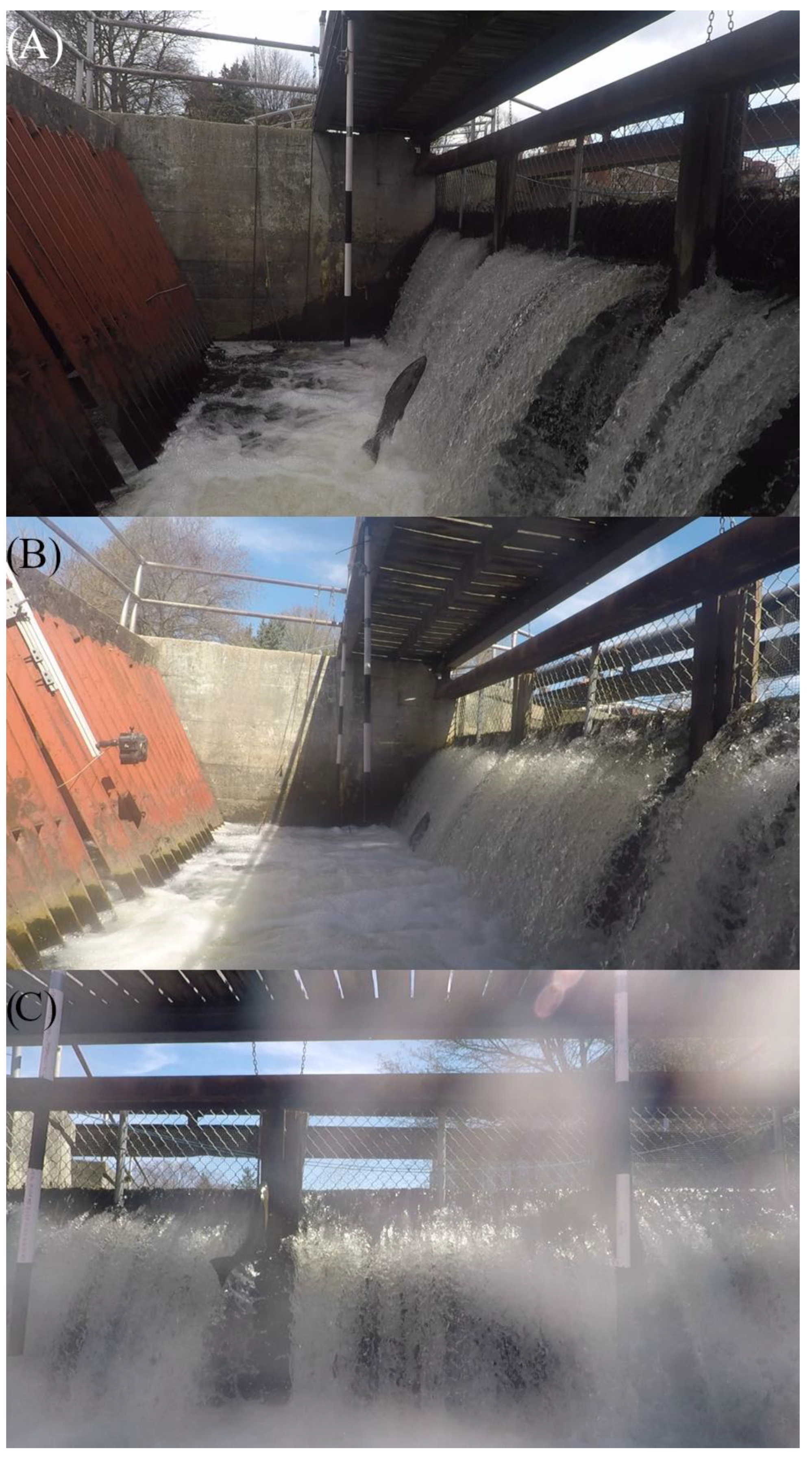
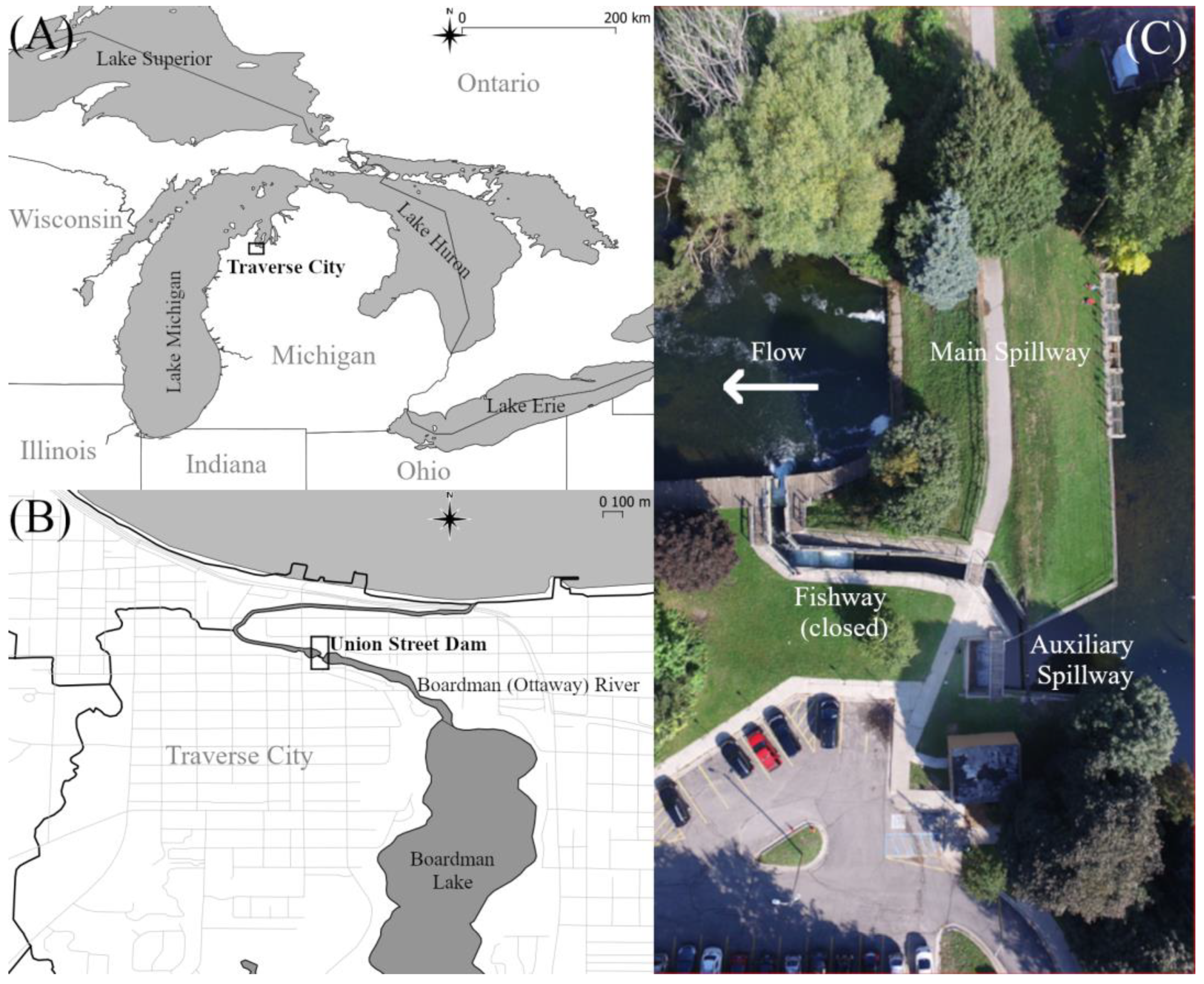
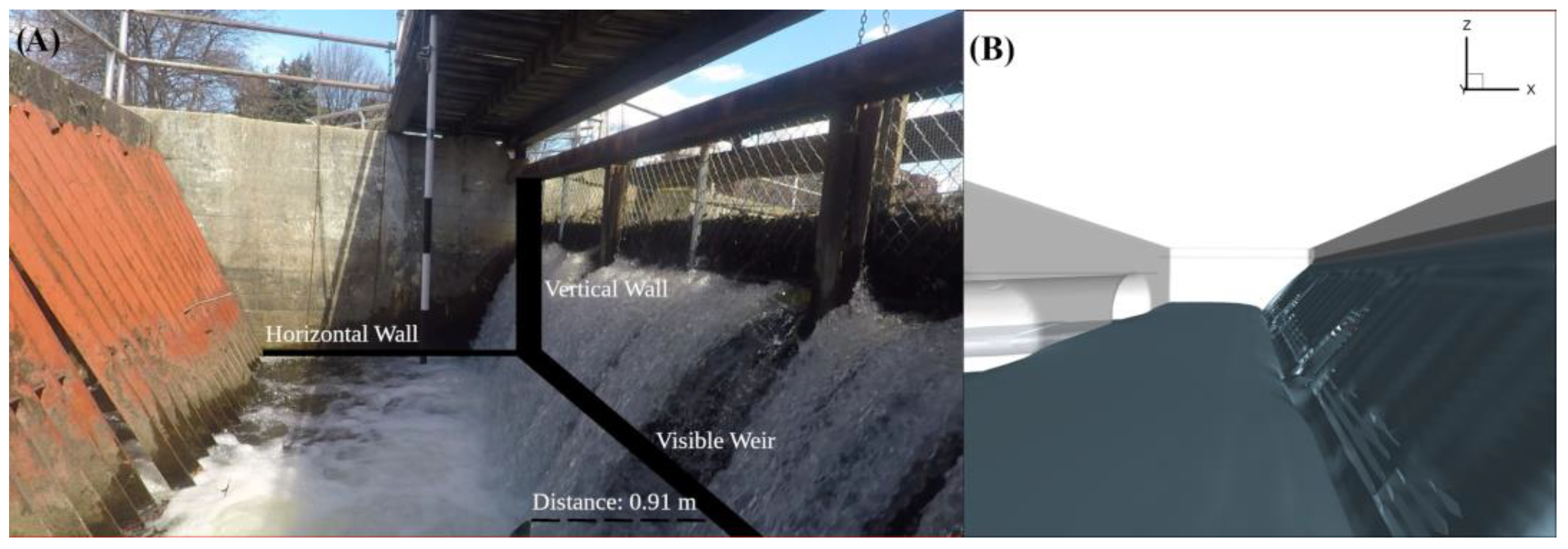
2.1. Field Site

The Union Street Dam (Traverse City, MI, USA) (44°55′41″ N, 85°37′21″ W) is located approximately 1.8 km upstream of West Grand Traverse Bay, Lake Michigan, on the Boardman (Ottaway) River. The dam operates as a run-of-river and maintains a normal pool elevation 179.7 m above sea level in the upstream impoundment. The flow through Union Street Dam is conveyed by the main spillway and auxiliary spillway. The main spillway consists of five 1.5 m L × 3.2 m W × 3.5 m D concrete bays, each with a stoplog weir and trash rack, and discharging into two 1.22 m diameter corrugated metal pipes. The auxiliary spillway consists of a single 3.6 m L × 5.6 m W × 2.9 m D concrete bay with a stoplog weir and discharging into two 1.22 m diameter corrugated metal pipes set at a slope of 4.5H:1V. The stoplog weir crest is set at 179.53 m. Water exits the pipes into a tailwater pool with an approximate depth of 1 m. The water temperatures during the data collection periods were 9.4 °C and 15.2 °C in 2022 and 2023, respectively.

2.2. Data Collection and Preprocessing

Data were collected in the auxiliary spillway (Figure 2) with a GoPro Hero 9 and recorded on a 128 GB microSD card. The camera recorded at a rate of 30 frames per second and a resolution of 2560 × 1440 using linear lens mode (i.e., 1440 p). During deployment, the camera recorded around 8 h of footage per day and deployment dates were selected to coincide with the spring migratory period for steelhead, ensuring fish were highly motivated to attempt passage over the spillway. Recordings were made only during the day and without precipitation to allow for unobstructed viewing.

In 2022, the camera was mounted downstream and perpendicular to the weir (camera 1 in Figure 2). It was placed 1.05 m below the top of the wall right to the weir and pointing slightly towards the nappe of the weir. A calibration stick was attached to the walkway above the weir and positioned perpendicular to the surface of the water and approximately 2.4 m from the camera (Figure 3A). The width of the channel at the weir measured approximately 5.6 m.

In 2023, two cameras were utilized. One camera was mounted in a similar position to that used in 2022, downstream and perpendicular to the weir. A second camera (camera 2 in Figure 2) was positioned downstream and facing the weir. The vantage point of the second camera enabled annotators to better gauge the depth of a jump and its trajectory (i.e., perpendicular to weir and parallel to weir) (Figure 3B,C). Two calibration sticks were attached to the walkway of the weir and positioned 2.67 m and 4.23 m from the camera, respectively. This placed the calibration sticks at roughly 45% and 72% of the width of the channel. With the second calibration stick, more jumps could be annotated as they were more likely to be in the proximity of a calibration stick. The calibration stick closest to the camera was not plumb and all launch angles which were calculated using this calibration stick were adjusted by 4 degrees.

The collected surveillance video was preprocessed to extract images of steelhead jumps through a two-stage process. First, VLC [36], a cross-platform media player, was used to scan the surveillance data and extract short clips of steelhead jumps. This resulted in 150 and 128 clips for spring 2022 and spring 2023, respectively. The shortened clips were then further processed with VLC to extract the individual frames contained in the video clips, saving them as PNG files.

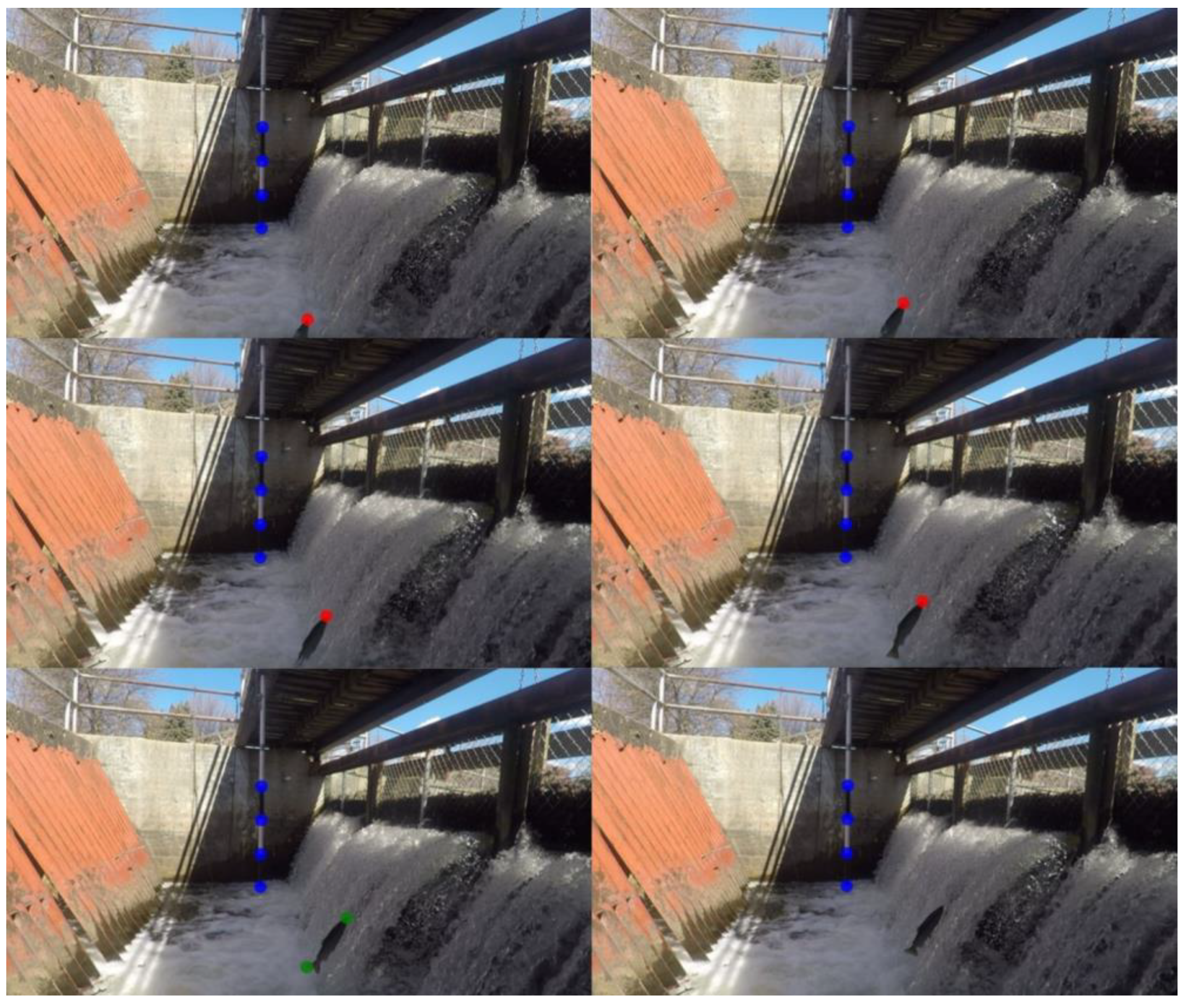
2.3. Image Annotation

To determine the launch angle, launch velocity, launch location, and fish length of each steelhead jump, a custom web application was developed and employed. The web application fulfilled three primary functions. First, the web application served the converted PNG images (i.e., extracted video frames) from the shortened surveillance clips, grouping the images by clip and presenting them individually in sequential order. This enabled the user to quickly identify frames for annotation. Second, the web application recorded the coordinates of key markers in the image (e.g., the position of the snout and the banding on the calibration stick), as indicated by the user. Finally, using the annotations, the program calculated the launch angle, launch speed, length of the fish, and distance from the weir.

As aforementioned, the web application provided access to relevant frames of collected video and assisted in annotating the locations of fish jumping in each video. Following the work of Morán-López and Uceda Tolosa [35], key markers which could determine the launch angle and speed of a jump were selected and a workflow was developed to capture the coordinates of these key markers through the web application. More specifically, the coordinates that were recorded from the frames were four pairs of coordinates indicating the position of the snout of a fish over four consecutive frames (with the first frame being the initial emergence of the snout), the tail of the fish, and the location of the four consecutive bands of the calibration stick (Figure 4). Additionally, the depth of the jump (i.e., estimated relative distance from the camera) was calculated from the key markers and recorded. Due to potential distortions in the camera lens, a conversion factor based on the distance between the fish and the camera (i.e., adjusting the pixels to meters conversion factor depending on the distance between the fish and the camera) was not interpolated. The distance between the fish and the camera (or depth of the jump with respect to the channel) was estimated so that only jumps near a calibration stick were analyzed. The depth of the jump and potential distortions in the camera lens would affect the fidelity of the conversion factor, with fidelity decreasing as a jump moves further away from a calibration stick. Thus, only jumps that were near a calibration stick were considered. Collectively, these data for a jump are referred to as an annotation (

Table 1. Data recorded for a jump annotation.

Name of Field	Sample Value for Field
Video file ID	63efd4cb5e1e50998c52e672
Start frame ID	63efd5385e1e50998c537129
Coordinate1	(747,164)
Coordinate2	(770,214)
Coordinate3	(791,263)
Coordinate4	(818,307)
Calibration1	(836,361)
Calibration2	(836,469)
Calibration3	(836,582)
Calibration4	(838,690)
Nose	(845,346)
Tail	(720,160)
Depth	35
Angle offset	0.12
Launch angle	65.41
Launch speed	3.76
Length	0.51
Annotated by	PN
Start Frame	BoardmanSpillway-2022-04-15-16h34m04s-GP102357-025.png
Video file name	BoardmanSpillway-2022-04-15-16h34m04s
Horizontal edge	883,381
Vertical edge	1,033,717
Visible weir coordinates	1,363,119
Distance from the wall	1.3

). The position of the tail and the calibration stick and the estimated jump depth were only recorded once per annotation. The launch angle, launch speed, length of the fish, and angle offset were all calculated using these coordinates. Due to the small tilt in the horizon of the camera, an angle offset was employed to adjust the calculations above.

2.4. Annotation Analysis

To determine the launch speed, the displacement of a fish in pixels was calculated using the Euclidean distance formula and then converted to meters through a conversion factor. To compute the conversion factor from pixels to meters, the pixel location of the start of the four bands on the calibration stick were considered and the average band length in pixels was calculated as shown in Equation (1). Given that the actual length of the bands was 0.25 m, the length of a band divided by the average pixel length yielded a conversion factor in meters/pixel. The displacement of the snout was also calculated from the coordinates from the remaining frames in the annotation, more specifically, the distance the snout traveled between each subsequent frame (i.e., between frame 1 and frame 2, between frame 2 and frame 3, etc.). Each distance was then multiplied by 30 to calculate the speed in meters per second as the camera was set to record at a rate of 30 frames per second. Of the speeds calculated for an annotation, the maximum speed was recorded by the web application. Finally, the pixel position of the tail and nose were identified, and the distance in pixels between the nose and the tail was calculated to obtain the length of the fish which was then converted to meters.

$${∆}_{pixel}=\sqrt{{\left(C_{x2}-C_{x1}\right)}^2+{\left(C_{y2}-C_{y1}\right)}^2},$$

(1)

where $C_x$ and $C_y$ are the coordinates of the calibration stick. The coordinates were also used to determine the angle offset of the frames as they all indicated some tilt from level. Equation (2) was used to calculate the angle offsets from calibration coordinates 2, 3, and 4. Then, the mean of these measurements was used to calculate the average angle offset, or the angle at which the image should be slanted to be plumb and level.

$${\theta }_{offset}={\tan }^{-1}\left(\frac{C_{y1}-C_{y0}}{C_{x1}-C_{x0}}\right)$$

(2)

To calculate the angle of emergence, the coordinates of the snout of a fish in the first two frames of its emergence from the water were utilized. Because the frames were skewed slightly due to the positioning of the camera, the angle offset was employed to account for this tilt in the angle of emergence using Equations (3) and (4). Equation (5) represents the calculation of the launch angle based on the transformed coordinates.

$$X^{\prime }=\left(\left(x_2-x_1\right)\cos {\theta }_{offset}\right)-\left(\left(y_2-y_1\right)\sin {\theta }_{offset}\right)$$

(3)

$$Y^{\prime }=\left(\left(y_2-y_1\right)\cos {\theta }_{offset}\right)+\left(\left(x_2-x_1\right)\sin {\theta }_{offset}\right)$$

(4)

$${\theta }_{launch}={\tan }^{-1}\left(\raisebox{1ex}{$Y^{\prime }$}\!\left/ \!\raisebox{-1ex}{$X^{\prime }$}\right.\right)$$

(5)

To estimate the distance from the weir as a fish emerged from the water, the line representing the base of the weir was determined using a portion of the weir which was visible through the curtain of water. This line was extrapolated over the length of the weir (Figure 5A). Then, a line was projected from the snout of the fish and parallel to the level of water on the opposing wall of the channel. The distance along this line from the snout of the fish to its intersection with the projected base of the weir was calculated in pixels and then converted to meters using a conversion factor.

As the depth of an object in the camera’s field of view affects its size in the image (i.e., objects further from the camera are represented by fewer pixels), annotated jumps were filtered by estimated depth from the camera. In 2022, the calibration stick was positioned approximately at 40% of the width of the channel and only jumps which were between 20–60% of the width of the channel were used for analysis. In 2023, an additional calibration stick and camera were deployed and this increased the coverage of the channel. Jumps ranging from 20 to 100% of the width of the channel were used for analysis.

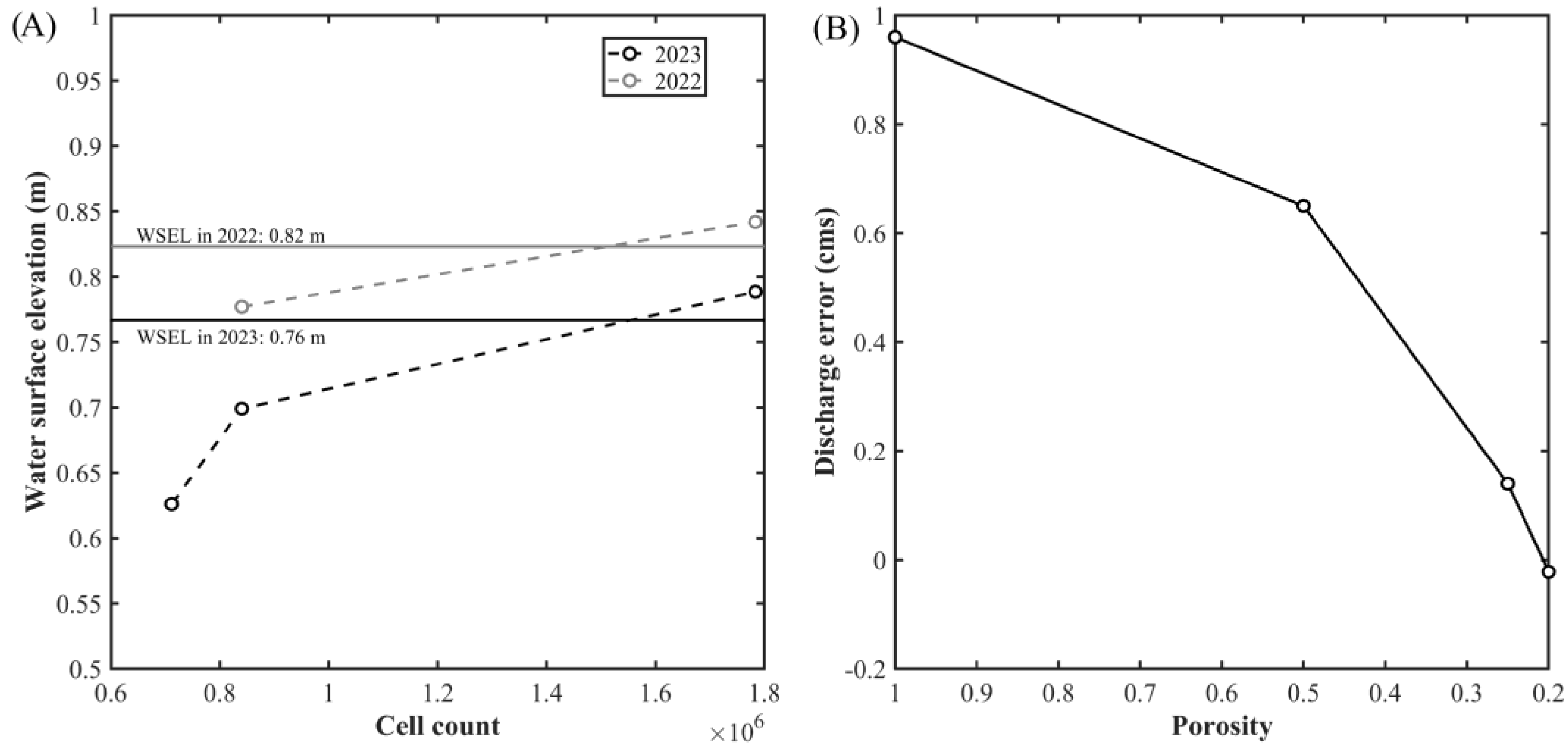
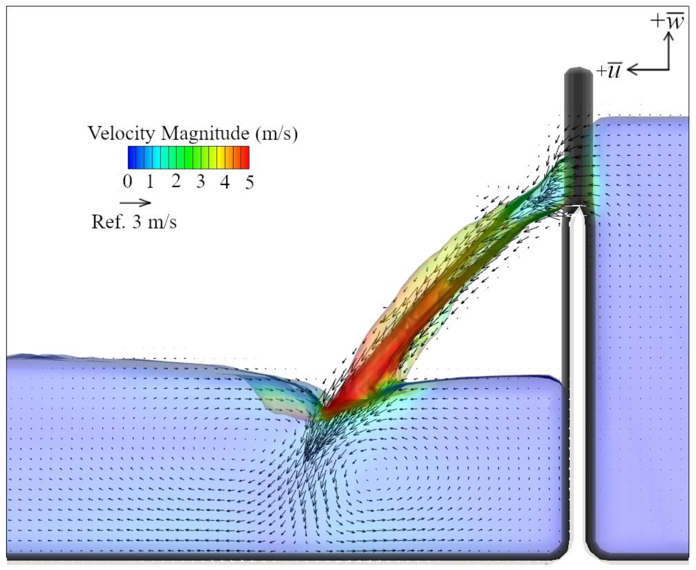
2.5. Hydraulic Modeling

The flow field in the Union Street Dam auxiliary spillway was modeled using FLOW-3D, version 12.0 (Flow-Science, Santa Fe, New Mexico), CFD code. To simulate turbulent flows, FLOW-3D solves the governing equations of motion for Newtonian incompressible flows (Equations (6) and (7)) using a finite volume method.

$$\frac{\partial {\overline{u}}_i}{\partial x_i}=0$$

(6)

$$\frac{\partial {\overline{u}}_i}{\partial t}+{\overline{u}}_i\frac{\partial {\overline{u}}_i}{\partial x_j}=g-\frac{1}{\rho }\frac{\partial P}{\partial x_j}+\nu \frac{{\partial }^2{\overline{u}}_i}{\partial x_j^2}-\frac{\partial }{\partial x_j}\left(\overline{{u_i}^{\prime }{u_j}^{\prime }}\right)$$

(7)

In Equations (6) and (7), $\rho$ is the density of the fluid, $g$ is the gravitational constant, $P$ is fluid pressure, $\nu$ is the kinematic viscosity, and the instantaneous velocity $u_i$ can be written as $u_i=\overline{u_i}+{u_i}^{\prime }$, where ${u_i}^{\prime }$ is the turbulent fluctuation of velocity and $\overline{u_i}$ is the time-averaged velocity. The velocity vector comprises velocities in the x-direction, $u$, y-direction, $v$, and z-direction, $w$. To close the system of equations in Equations (6) and (7), a two-equation turbulence model is used. In this study, the Renormalization Group (RNG) $k-\epsilon$ model was selected because it has wider applicability than the standard $k-\epsilon$ model [37,38] and better handles a low Reynolds number and near-wall flows. A first-order upwind approximation scheme was employed for the momentum advection equations, and an implicit generalized minimum residual method solver was used to determine cell pressures and update the velocity field. The free water surface was tracked using the volume-of-fluid method.

Solid geometry of the auxiliary spillway was generated from detailed construction drawings using AutoCAD 2020 (Autodesk, San Rafael, CA, USA) (Figure 2). Discretization of the geometry and mesh development were completed using FAVOR (Fractional Area-Volume Obstacle Representation), which is built into FLOW-3D. The computational mesh was constructed of three uniform mesh blocks: an upstream block (#1) used a 4.5 cm cell size, the middle block (#2) used a 7.6 cm cell size, and the downstream block (#3) used a 10 cm cell size (Figure 2). The mesh contained all rectangular prisms. To test for grid convergence, three progressively finer mesh sizes were evaluated and the water surface elevation within the pool below the stoplogs was compared to field values (Figure 6A). The finest mesh containing 1.7 M cells was used for all further calculations. Upstream and downstream boundary conditions were specified as a constant water surface elevation based on data collected from water level probes with hydrostatic pressure distributions. Specifying the water elevation allows flow rate in the spillway to adjust according to flow control at the stoplogs. A chain-link fence panel sits on top of the stoplogs to prevent fish passage. Since the fence panel collects debris and limits the discharge capacity of the auxiliary weir, the fence panel was modeled as a porous surface [39]. To determine what porosity was appropriate for the fence panel, an exploratory analysis of CFD-modeled data was compared to discharge measurements taken at the Union Street Dam. Discharge measurements were taken at the downstream end of the spillway on 23 May 2023. During measurements, the average discharge through the auxiliary spillway was 0.56 cm. Several CFD models were run, each with a different porosity value (1, 0.5, 0.25, and 0.2), and the simulated discharge through each model was then compared to the field measurement (Figure 6B). The model that best fit the field measurements used a porosity in all directions of 0.20.

A total of two flow scenarios were run, one for each year of steelhead leaping video capture. Each model assumed a constant headwater and tailwater level as recorded by water level gauges located ~3 m upstream of the stoplogs and ~50 m downstream of the spillway (

Table 2. Summary of the boundary conditions used for each computational fluid dynamics simulation.

Date	US WSEL (m)	DS WSEL (m)	Calculated Discharge (cm)
15 April 2022	179.82	176.4	0.85
14 April 2023	179.79	176.4	0.78

). Each CFD model was run until it reached a quasi-steady state in which the total fluid volume within the computational domain reached a plateau. A quasi-steady state was reached within 200 s of flow time with a coarse mesh (one half of the total mesh size) so the flow field would reach an initial flow for a finer mesh. The fine mesh models simulated 100 s of flow time with the hydraulic output saved every ten seconds of flow time. Preliminary post-processing of CFD data was conducted using TecPlot 360 (TecPlot, Bellevue, Washington, DC, USA) to extract the velocity vectors along the centerline of the spillway (Figure 5B).

For each flow scenario, the difference angle, ${\theta }_{diff}$, between each fish launch angle and direction of the velocity vector were calculated as

$${\theta }_{diff}=\left|{\theta }_{launch}-{\theta }_{flow}\right|,$$

(8)

where ${\theta }_{flow}$ is the mean direction of the velocity vector in the xz-plane in the upper half of the water column calculated along the centerline of the spillway at the point each jump was initiated.

2.6. Statistical Analyses

To assess the impact of observer variability, all jumps were annotated by two members of the research team. Then, a series of paired t-tests were performed on the calculated values for launch angle, launch velocity, length, and distance from the spillway crest. Next, to determine any potential relationships between jump characteristics, the Pearson correlation coefficient was calculated between the normalized launch speed (i.e., launch speed/length of fish) and launch angle and between fish length and launch speed. Independent t-tests were also performed to assess the differences in mean launch angle, mean launch speed, and mean fish length across the two collection seasons.

The analysis of leaping difference angle was analyzed using a Generalized Linear Mixed Model (GLMM). To ensure normality, the dependent variable, difference angle, was transformed using a Box-Cox Transformation [40], with an optimal lambda of 0.7249. The transformed difference angle was analyzed using the velocity magnitude and normalized leaping speed as the fixed effects and the year as a random effect. The linear regression and normality assumptions were explored using Pearson model residuals. The histogram of the model residuals was normally distributed at about zero and a plot of normalized residuals against the fitted values did not indicate a systematic dependence of the variance on the fitted values. Examining the residual lag plots did not reveal signs of the possible non-independence of observations from the unmodeled autocorrelated processes [41]. We further considered reduced models with all possible combinations of fixed effects. To determine which model was best supported by the data, an information theoretic approach was performed using Akaike’s information criterion (AIC), where the model with the lowest AIC value was the best model. The data were analyzed using the fitglme function in MATLAB.

3. Results

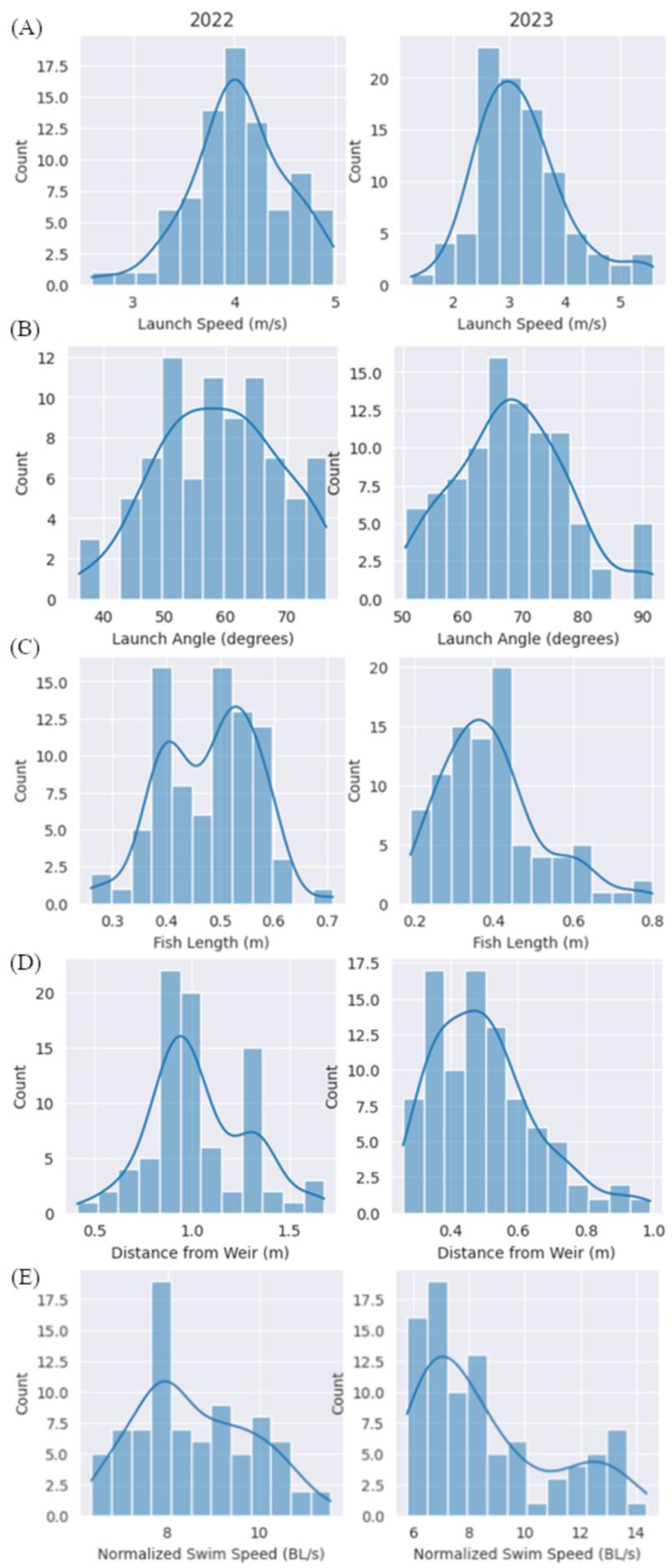
3.1. Jump Characteristics

Launch angle, launch speed (normalized by body length and absolute), fish length, and distance from the crest were calculated for 173 jumps (83 in 2022 and 90 in 2023) at the auxiliary spillway of the Union Street Dam (

Table 3. Summary statistics (mean ± standard deviation) of launch speed (normalized by body length and absolute), launch angle, distance from crest, and fish length for 2022 and 2023 annotations.

	Launch Speed
Year	Absolute (m/s)	Normalized (BL/s)	Launch Angle (°)	Fish Length (m)	Distance from Crest (m)
2022	4.05 ± 0.46	8.60 ± 1.25	58.73 ± 9.88	0.48 ± 0.09	1.03 ± 0.25
2023	3.24 ± 0.81	8.61 ± 2.42	68.2 ± 9.5	0.40 ± 0.13	0.50 ± 0.15

; Figure 7) (Raw data available in Tables S1 and S2). Differences in mean absolute launch speed (t = 8.29, p << 0.001), mean launch angle (t = −6.49, p << 0.001), mean fish length (t = 5.38, p << 0.001), and distance from the crest (t = 16.97, p << 0.001) were evident between data collected in 2022 and 2023; however, no significant year effect was found for the normalized launch speed (t = −0.051, p = 0.95). No significant relationship was found between the normalized launch speed and launch angle (r = 0.11 and r = 0.12, for 2022 and 2023, respectively).

3.2. Observer Variability

In 2022, there were 68 paired annotations and the results of the paired t-test did not indicate any significant differences in launch speed (t = 1.493; p = 0.140), launch angle (t = 0.495; p = 0.622), or fish length (t = −1.361; p = 0.178). However, a significant difference was found for distance from the crest (t = 4.078; p = 0.0001) (Table S3).

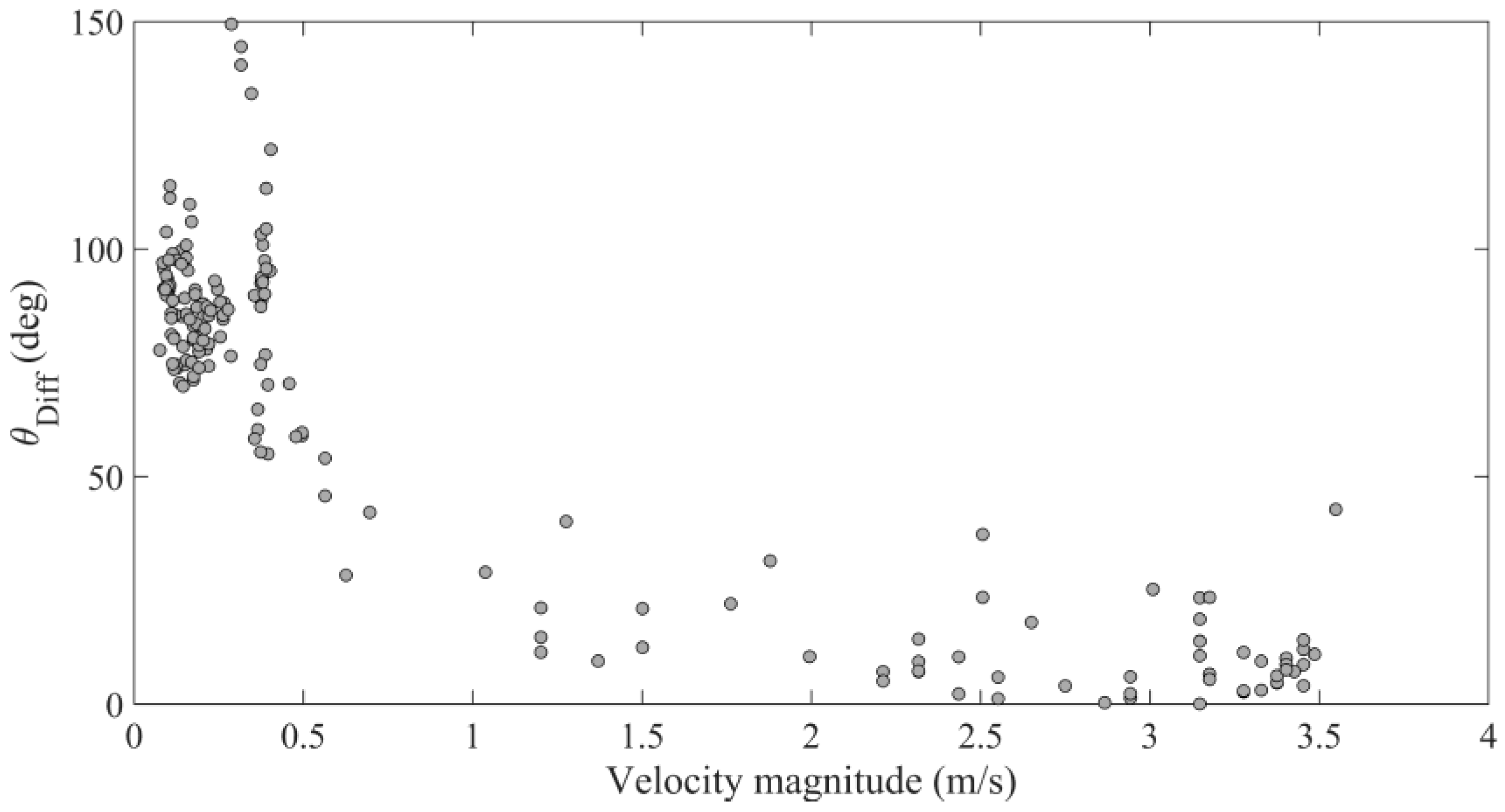
3.3. Hydraulic Conditions and Difference Angle

Hydraulic conditions in the Union Street Dam auxiliary spillway were typical of a sharp crested weir. The water depth in the pool was 0.82 m and 0.76 m in 2022 and 2023, respectively. Due to the reduction in discharge capacity caused by debris on the fence panel, the water surface profile of the plunging water does not directly connect with the upstream water surface, indicating a head loss of approximately 20 cm. The flow pattern in the spillway pool was typical of pool and weir fishways with zones of recirculation on each side of the plunging jet (Figure 8). Velocity magnitudes in the center of the plunging jet exceed 5 m/s and quickly dissipate to less than 1 m/s in the surrounding pool. The mean angle of the velocity vector at the center of the plunging jet was 56.64° and 48.55° (CCW from horizontal) for 2022 and 2023, respectively.

The model most supported by the data contained velocity magnitude and year as a random factor (

Table 4. List of model and AIC scores for Generalized Linear Mixed Model of difference angle. Model variables with fixed effects include velocity magnitude (VM) and launch speed (LS), while year was modeled as a random effect.

Model	AIC	ΔAIC
VM + (Year)	101.17	-
VM + LS + (Year)	102.48	1.31
LS + (Year)	320.42	219.25

). While the model including launch speed had a marginal increase in AIC score, the covariate was not statistically significant. Velocity magnitude was positively associated with the difference angle (

Table 5. Fixed effects from the top Generalized Linear Mixed Model to explain the difference angle between fish leaping angle and velocity vector. The R-square value for the top model is 0.82.

Model Term	Coefficient	SE	df	t	p-Value
Intercept	0.549	0.032	171	17.4	<<0.05
Velocity Magnitude	−0.524	0.020	171	−27.0	<<0.05

). There is a clear tendency for the difference angle to trend towards zero when the velocity magnitude exceeds 0.5 m/s (Figure 9).

4. Discussion

4.1. Comparison of Jump Characteristics

The mean launch angle derived in this study was comparable to that obtained in prior studies of the jumping behavior of Pacific salmonids [16,32] and falls within the range examined by Powers and Osborn [24]. The normalized launch speed was also consistent with the maximum swim speed of similar sized steelhead observed by Weaver [29], but almost 2 BL/s faster than expected from the data collected by Katapodis and Gervais [30]. For the intended use to inform evaluations of passage, launch speed characteristics collected from fish jumping observations are preferable to estimates from swimming performance tests. Swim tunnel tests often underestimate maximum, or burst, swimming speeds due to space restrictions and limited motivation [42,43]. While the water temperature during data collection fell within the lower limit anticipated for steelhead to reach their maximum attainable swim speed [31], steelhead entering later in the migratory season with presumably warmer water temperatures could possibly reach higher launch speeds. Additionally, the lack of difference in the normalized launch speed between years would suggest that 8.6 BL/s is a reasonable estimate of the average normalized launch speed for Great Lakes steelhead. These data could be useful for design purposes but careful attention should be paid to the extremes as one individual reached 14 BL/s on one attempt.

The water depth in the pool below the barrier was approximately 1.8 times the mean body length, suggesting that launch angle and launch speed were likely not restricted by water depth. However, the ratio of pool depth to fall height, 0.75, was less than the minimum recommended ratio for inducing salmonid jumping behaviors [16,33]. It is yet unclear if similar characteristics would be observed in a natural setting, as the test site was an engineered structure lacking a defined plunge pool that would typically be associated with a waterfall (e.g., natural passage barrier).

Leaping attempts away from the calibration stick or with a trajectory out of the plane perpendicular to the stoplogs were not utilized in this analysis. As a result, only 62% of available leap attempts were considered. This restriction minimized the potential error caused by changes in the distance between the fish and the camera and simplified the integration of leap characteristics with CFD analysis. Due to the simplistic geometry of the auxiliary spillway, the velocity fields were dominated by flow structures in the streamwise direction (e.g., the plane perpendicular to the stoplogs) and, thus, were the most likely cues of leaping behavior. Certainly, out of plane trajectories may be important to quantify at barriers with more complex, fully three-dimensional flow fields.

4.2. Hydraulic Cues of Launch Angle

Previous studies suggest that the leaping angle is dependent on the location of the standing wave resulting from a falling jet of water [24,33,34]. In the event a standing wave forms downstream of the falling jet of water, the vertical component of the water velocity can aid launch speed. However, a pronounced standing wave was not present at this site, nor were jump attempts located within the region a standing wave would be expected. In fact, most jump attempts were made between the jet and the crest in 2023. While this study did not investigate the possibility that other hydraulic characteristics could influence launch angle, the trend observed between the difference angle and velocity magnitude (Figure 9) provides compelling evidence that simple mean flow direction is a predominate cue for launch angle selection.

The CFD modeling approach used in this study results in simulated flow fields that are essentially time-averaged, and ephemeral features of flow were not considered. Other CFD solutions, such as Large-eddy Simulation (LES), permit solution of instantaneous flow fields that contains hydraulic structures (e.g., eddies) with more transient characteristics that may influence different leaping behaviors over time. However, there are currently no methods available to sync time-variant LES solutions to those experienced by fish in their natural environment [44]. As a result, our approach used spatial and temporal averaging to account for the inherent uncertainty between linking observed movements in the field to the simulated environment. Indeed, more precise examination of higher order fish movement and transient flow conditions would likely yield clearer insights to fish leaping behavior, but such an effort would require more controlled conditions and instrumentation that would be better suited for laboratory settings.

While this field study benefits from the innate motivation of natural migratory movements, conditions prevented further clarification of fish swimming trajectories prior to jumping (i.e., underwater video). Thus, hydraulic characteristics used in this analysis were averaged over the upper half of the water column and not directly measured along the fish swim path. Regardless, the finding that the difference angle is minimized as velocity increases appears reasonable as velocity magnitude reaches its maximum at the center of the falling jet and the flow direction could be used by fish to estimate the required launch angle. It is plausible that fish would attempt to mimic the trajectory of the falling jet as it would provide the most likely opportunity to jump over the barrier. Launch angles that are more oblique would result in jumps that fall short of the barrier while more acute launch angles may not reach the requisite height to overcome the barrier.

This study could not control for replication, as the video capture did not discern individual fish making multiple jump attempts. While replication does not negatively influence development and use of the web application for image processing, it does place some caveats on the resulting data. It is possible that the data could be dominated by just a few individuals, but the range of fish lengths (Figure 7) would suggest this effect is limited, as at least seven different size classes contributed at least five jumps in each year. Despite the lack of control for replication, the leap characteristics are within the range expected from the literature and thus, are a likely a reasonable representation of the population of steelhead migrating in the Boardman River in the spring.

4.3. Additional Uses of Custom Annotation Application

The web application and instructions for its use are provided on OSF at https://doi.org/10.17605/OSF.IO/5HRFK. It could readily be modified to calculate other distances (e.g., width or distance traveled) or waypoints from successive frames of video. Shapes within a single frame could be traced to calculate area. More immediate applications would be characterizing leaps of other species of fish or at other collection sites. The key to these calculations will be a consistent depth in the field of view of the camera and an appropriately placed calibration stick. This web application is yet another example of how computer vision techniques could be used to enhance routine fisheries measurements [45] and even imaged-based fish sorting [46].

5. Conclusions

This study presented a custom web application developed to semi-automate the annotation process, enabling faster and more efficient data collection for fish leaping characteristics. Data collection took place during migratory runs in the spring of 2022 and 2023 that resulted in 173 total leaps annotated with mean launch angles of 58.73° and 68.2°, in 2022 and 2023, respectively. The mean launch speed normalized by body length was consistent across years at 8.6 body lengths per second. The integration of leaping data with computational fluid dynamics simulations revealed steelhead launch angle aligns closely with the water velocity direction as the velocity magnitude increases. The web application tool and data collected will support the unintended passage hazard analysis at FishPass, a facility that will replace the Union Street Dam with a new barrier with selective fish passage capabilities and could help inform future design of selective fishways in the Great Lakes basin [20]. These findings provide valuable insights into the behavior of steelhead and contribute to the ongoing efforts to manage their passage in the Great Lakes basin. Future research could explore the application of the web-based annotation tool to other species and other river systems.

References

1. Lovell, S.J.; Stone, S.F.; Fernandez, L. The Economic Impacts of Aquatic Invasive Species: A Review of the Literature. Agric. Resour. Econ. Rev. 2006, 35, 195–208. [Google Scholar] [CrossRef]
2. Coble, D.W.; Bruesewitz, R.E.; Fratt, T.W.; Scheirer, J.W. Lake Trout, Sea Lampreys, and Overfishing in the Upper Great Lakes: A Review and Reanalysis. Trans. Am. Fish. Soc. 1990, 119, 985–995. [Google Scholar] [CrossRef]
3. Fetterolf, C.M., Jr. M. Why a Great Lakes Fishery Commission and Why a Sea Lamprey International Symposium. Can. J. Fish. Aqua. Sci. 1980, 37, 1588–1593. [Google Scholar] [CrossRef]
4. McLaughlin, R.L.; Smyth, E.R.; Castro-Santos, T.; Jones, M.L.; Koops, M.A.; Pratt, T.C.; Vélez-Espino, L.-A. Unintended consequences and trade-offs of fish passage. Fish Fish. 2013, 14, 580–604. [Google Scholar] [CrossRef]
5. Siefkes, M.J.; Steeves, T.B.; Sullivan, W.P.; Twohey, M.B.; Li, W. Sea Lamprey Control: Past, Present, and Future. In Great Lakes Fisheries Policy and Management: A Binational Perspective, 2nd ed.; Taylor, W.W., Lynch, A.J., Leonard, N.J., Eds.; Michigan State University Press: East Lansing, MI, USA, 2013; pp. 651–704. [Google Scholar]
6. Zielinski, D.P.; McLaughlin, R.; Castro-Santos, T.; Paudel, B.; Hrodey, P.; Muir, A. Alternative sea lamprey barrier technologies: History as a control tool. Rev. Fish. Sci. Aqua 2019, 27, 438–457. [Google Scholar] [CrossRef]
7. Lake Michigan’s Tributary and Nearshore Fish Habitats. Available online: https://www.researchgate.net/publication/242113783_Lake_Michigan’s_tributary_and_nearshore_fish_habitats (accessed on 2 October 2022).
8. Lane, J.A.; Portt, C.B.; Minns, C.K. Nursery Habitat Characteristics of Great Lakes Fishes; Can. MS Rpt. Fish. Aquati. Sci. 2338; Fisheries and Oceans Canada: Ottawa, ON, Canada, 1996; pp. 1–44. [Google Scholar]
9. River Renewal: Restoring Rivers Through Hydropower Dam Relicensing|Hydropower Reform Coalition. Available online: https://hydroreform.org/resource/river-renewal-restoring-rivers-through-hydropower-dam-relicensing/ (accessed on 3 April 2023).
10. Williams, J.G.; Amstrong, G.; Katopodis, C.; Larinier, M.; Travade, F. Thinking like a fish: A key ingredient for development of effective fish passage facilities at river obstructions. River Res. App. 2012, 28, 407–417. [Google Scholar] [CrossRef]
11. Mallen-Cooper, M.; Brand, D.A. Non-salmonids in a salmonid fishway: What do 50 years of data tell us about past and future fish passage? Fish. Manag. Ecol. 2007, 14, 319–332. [Google Scholar] [CrossRef]
12. Bunt, C.M.; Castro-Santos, T.; Haro, A. Reinforcement and validation of the analyses and conclusions related to fishway evaluation data from Bunt et al.:‘Performance of fish passage structures at upstream barriers to migration’. River Res. App. 2016, 32, 2125–2137. [Google Scholar]
13. Clay, C.H.; Eng, P. Design of Fishways and Other Fish Facilities, 1st ed.; CRC Press: Boca Raton, FL, USA, 2017; pp. 1–247. [Google Scholar]
14. Buysse, D.; Coeck, J.; Maes, J. Potential re-establishment of diadromous fish species in the River Scheldt (Belgium). Hydrobiologia 2008, 602, 155–159. [Google Scholar] [CrossRef]
15. Kareiva, P.; Marvier, M.; McClure, M. Recovery and management options for spring/summer chinook salmon in the Columbia River basin. Science 2000, 290, 977–979. [Google Scholar] [CrossRef]
16. Lauritzen, D.V.; Hertel, F.S.; Jordan, L.K.; Gordon, M.S. Salmon jumping: Behavior, kinematics and optimal conditions, with possible implications for fish passageway design. Bioinspir. Biomim. 2010, 5, 035006. [Google Scholar] [CrossRef]
17. Lundqvist, H.; Rivinoja, P.; Leonardsson, K.; McKinnell, S. Upstream passage problems for wild Atlantic salmon (Salmo salar L.) in a regulated river and its effect on the population. Hydrobiologia 2008, 602, 111–127. [Google Scholar] [CrossRef]
18. Stuart, I.G.; Marsden, T.J. Evaluation of cone fishways to facilitate passage of small-bodied fish. Aquac. Fish. 2019, 6, 125–134. [Google Scholar] [CrossRef]
19. Silva, A.T.; Lucas, M.C.; Castro-Santos, T.; Katopodis, C.; Baumgartner, L.J.; Thiem, J.D.; Cooke, S.J. The future of fish passage science, engineering, and practice. Fish Fish. 2018, 19, 340–362. [Google Scholar] [CrossRef]
20. Zielinski, D.P.; McLaughlin, R.L.; Pratt, T.C.; Goodwin, R.A.; Muir, A.M. Single-stream recycling inspires selective fish passage solutions for the connectivity conundrum in aquatic ecosystems. Bioscince 2020, 70, 871–886. [Google Scholar] [CrossRef] [PubMed]
21. Benoit, D.M.; Zielinski, D.P.; Swanson, R.G.; McLaughlin, R.L.; Castro-Santos, T.R.; Goodwin, R.A.; Pratt, T.C.; Muir, A.M. FishPass sortable attribute database: Phenological, morphological, physiological, and behavioral characteristics related to passage and movement of Laurentian Great Lakes fishes. J. Great Lakes Res. 2023. [Google Scholar] [CrossRef]
22. Zorn, T.G.; Hessenauer, J.M.; Wills, T.C. Increasing connectivity of Great Lakes tributaries: Interspecific and intraspecific effects on resident brook trout and brown trout populations. Ecol. Freshw. Fish. 2019, 29, 519–532. [Google Scholar] [CrossRef]
23. Reiser, D.W.; Huang, C.M.; Beck, S.; Gagner, M.; Jeanes, E. Defining flow windows for upstream passage of adult anadromous salmonids at cascades and falls. Trans. Am. Fish. Soc. 2006, 135, 668–679. [Google Scholar] [CrossRef]
24. Powers, P.D.; Osborn, J.F. New Concepts in Fish Ladder Design: Analysis of Barrier to Upstream Fish Migration, Volume IV of IV; Investigation of the Physical and Biological Conditions Affecting Fish Passage Success at Culverts and Waterfalls. 1982-1984 Final Report, Contract DE-A179-82BP36523, Project 82–14, USA. 1985. Available online: http://www.efw.bpa.gov/Publications/U36523–1.pdf (accessed on 18 December 2018).
25. Zielinski, D.P.; Freiburger, C. Advances in fish passage in the Great Lakes basin. J. Great Lakes Res. 2021, 47, S439–S447. [Google Scholar] [CrossRef]
26. Scott, W.B.; Crossman, E.J. Freshwater Fishes of Canada. Fish. Res. Board Can. Bull. 1973, 1, 1–966. [Google Scholar]
27. Biette, R.M.; Dodge, D.P.; Hassinger, R.L.; Stauffer, T.M. Life History and Timing of Migrations and Spawning Behavior of Rainbow Trout (Salmo gairdneri) Populations of the Great Lakes. Can. J. Fish. Aqua. Sci. 1981, 38, 1759–1771. [Google Scholar] [CrossRef]
28. Goodyear, C.D.; Edsall, T.A.; Dempsey, D.O.; Moss, G.D.; Polanski, P.E. Atlas of the Spawning and Nursery Areas of Great Lakes Fishes; Volume VIII; FWS/OBS-82/52; U.S. Fish and Wildlife Service: Washington, DC, USA, 1982; pp. 1–144. [Google Scholar]
29. Weaver, C. Influence of water velocity upon orientation and performance of adult migrating salmonids. U.S. Fish Wildl. Serv. Fish. Bull. 1963, 63, 97–121. [Google Scholar]
30. Katopodis, C.; Gervais, R. Fish Swimming Performance Database and Analyses; Research Document 2016/002; Fisheries and Oceans Canada: Ottawa, ON, Canada, 2016; p. 550. [Google Scholar]
31. Webb, P.W. Temperature effects on acceleration of rainbow trout, Salmo gairdneri. J. Fish. Res. Board. Can. 1978, 35, 1417–1422. [Google Scholar] [CrossRef]
32. Lauritzen, D.V.; Hertel, F.S.; Gordon, M.S. A kinematic examination of wild sockeye salmon jumping up natural waterfalls. J. Fish. Biol. 2005, 67, 1010–1020. [Google Scholar] [CrossRef]
33. Stuart, T.A. The leaping behaviour of salmon and trout at falls and obstructions. Freshw. Salmon Fish. Res. 1962, 28, 1–46. [Google Scholar]
34. Aaeserude, R.G.; Osborn, J.F. New Concepts in Fish Ladder Design, Volume II of IV.; Results of Laboratory and Field Research on New Concepts in Weir and Pool Fishways. 1982–1984 Final Report, Contract DE-AI79-82BP36523, Project 82-14, USA. 1985. Available online: https://www.osti.gov/servlets/purl/5965536 (accessed on 18 December 2018).
35. Morán-López, R.; Uceda-Tolosa, Ó. Biomechanics of fish swimming and leaping under waterfalls: A realistic field, image-based biophysical model with bioengineering implications. Bioinspir. Biomim. 2020, 15, 056011. [Google Scholar] [CrossRef] [PubMed]
36. VLC: Official Site—Free Multimedia Solutions for all OS!—VideoLAN. Available online: https://www.videolan.org/ (accessed on 4 January 2023).
37. FLOW-3D. FLOW-3D User Manual. Flow Science Inc. Available online: https://flow3d.sharefile.com/share/view/scc68be45df33406698c1b39eee7d3b14 (accessed on 14 September 2023).
38. Pope, S.B. Turbulent Flows; Cambridge University Press: Cambridge, UK, 2000; p. 771. [Google Scholar]
39. Ho, J.; Coonrod, J.; Hanna, L.J.; Mefford, B.W. Hydrodynamic modelling study of a fish exclusion system for a river diversion. River Res. Applic. 2011, 27, 184–192. [Google Scholar] [CrossRef]
40. Box, G.E.P.; Cox, D.R. An analysis of transformations. J. Roy. Stat. Soc. Ser B 1964, 26, 211–252. [Google Scholar] [CrossRef]
41. Silva, A.T.; Hatry, C.; Thiem, J.D.; Gutowsky, L.F.G.; Hatin, D.; Zhu, D.Z.; Dawson, J.W.; Katopodis, C.; Cooke, S.J. Behaviour and locomotor activity of a migratory catostomid during fishway passage. PLoS ONE 2015, 10, 0123051. [Google Scholar] [CrossRef]
42. Tudorache, C.; O’Keefe, R.A.; Benfey, T.J. Flume length and post-exercise impingement affect anaerobic metabolism in brook charr Salvelinus fontinalis. J. Fish Biol. 2010, 76, 729–733. [Google Scholar] [CrossRef]
43. Tudorache, C.; Viaenen, P.; Blust, R.; De Boeck, G. Longer flumes increase critical swimming speeds by increasing burst and glide swimming duration in carp (Cyprinus carpio L.). J. Fish Biol. 2007, 71, 1630–1638. [Google Scholar] [CrossRef]
44. Goodwin, R.A.; Lai, Y.G.; Taflin, D.E.; Smith, D.L.; McQuirk, J.; Trang, R.; Reeves, R. Predicting near-term, out-of-sample fish passage, guidance, and movement across diverse river environments by cognitively relating momentary behavioral decisions to multiscale memories of past hydrodynamic experiences. Front. Ecol. Evol. 2023, 11, 703946. [Google Scholar] [CrossRef]
45. Bravata, N.; Kelly, D.; Eickholt, J.; Bryan, J.; Miehls, S.; Zielinski, D. Applications of deep convolutional neural networks to predict length, circumference, and weight from mostly dewatered images of fish. Ecol. Evol. 2020, 10, 9313–9325. [Google Scholar] [CrossRef] [PubMed]
46. Eickholt, J.; Kelly, D.; Bryan, J.; Miehls, S.; Zielinski, D. Advancements towards selective barrier passage by automatic species identification: Applications of deep convolutional neural networks on images of dewatered fish. ICES J. Mar. Sci. 2020, 77, 2804–2813. [Google Scholar] [CrossRef]
Figure 1. (A) Map of Great Lakes region; (B) map of Traverse City, MI and location of the Union Street Dam on the Boardman (Ottaway) River; (C) Union Street Dam and water conveyance structures.
Fishes 08 00476 g001
Figure 2. View of the auxiliary spillway geometry: (A) isometric view of the spillway with approximate locations of cameras and computational fluid dynamics mesh blocks noted, and (B) cross-sectional view of the auxiliary spillway where fish were observed.
Fishes 08 00476 g002
Figure 3. Image of a steelhead attempting to traverse the weir collected by (A) camera 1 on 15 April 2022; (B) camera 1 on 14 April 2023; and (C) camera 2 on 14 April 2023. Note the calibration sticks are visible in all images.
Fishes 08 00476 g003
Figure 4. Illustration of recorded markers over six consecutive frames. The blue circles indicate markers on the calibration staff, the red circle indicates the snout of the fish, and green circles indicate are used to calculate the length of the fish.
Fishes 08 00476 g004
Figure 5. (A) Inferred lines used to estimate jump distance from weir crest and (B) simulated water surface from the CFD model.
Fishes 08 00476 g005
Figure 6. (A) Grid convergence evaluation and comparison of water surface elevation in the pool downstream of the stoplogs, and (B) calibration of screen porosity and the difference between calculated discharge and observed.
Fishes 08 00476 g006
Figure 7. Distribution of (A) absolute launch speed, (B) launch angle, (C) fish length, (D) distance from weir, and (E) normalized swim speed from 2022 and 2023 observations.
Fishes 08 00476 g007
Figure 8. Contours of the velocity magnitude and velocity vectors along the centerline of the auxiliary spillway for the 2023 flow scenario. Arrows in the upper right indicate positive direction for u ¯ and w ¯ velocity vectors.
Fishes 08 00476 g008
Figure 9. Scatter plot of difference angle against velocity magnitude for each jump.
Fishes 08 00476 g009