Article

Juvenile Hake Merluccius gayi Spatiotemporal Expansion and Adult-Juvenile Relationships in Chile

by
Daniela V. Yepsen
1,
Luis A. Cubillos
1,2,* and
Hugo Arancibia
1
1
Programa de Doctorado en Ciencias mención Manejo en Recursos Acuáticos Renovables, Facultad de Ciencias Naturales y Oceanográficas, Universidad de Concepción, Concepción 4070386, Chile
2
Centro COPAS COASTAL, Departamento de Oceanografía, Facultad de Ciencias Naturales y Oceanográficas, Universidad de Concepción, Casilla 160-C, Concepción 4070386, Chile
*
Author to whom correspondence should be addressed.
Fishes 2022, 7(2), 88; https://doi.org/10.3390/fishes7020088
Submission received: 23 February 2022 / Revised: 30 March 2022 / Accepted: 6 April 2022 / Published: 12 April 2022
(This article belongs to the Section Biology and Ecology)

Abstract

:
The abundance of juvenile fish changes due to endogenous processes, and determining the functional relationships among conspecifics is essential for fisheries’ management. The hake (Merluccius gayi) is an overexploited demersal fish widely distributed in Chile, from 23°39′ S to 47°00′ S in shallow and deep water over the continental shelf and shelf break. We studied the spatiotemporal distribution of hake juveniles (from ages 0 and 1), emphasizing endogenous relationships among juveniles and adults. The abundance per age data were obtained from bottom trawl cruises carried out in the austral winter between 1997 and 2018. Generalized additive models showed a similar spatiotemporal pattern for ages between 0 and 1, and negative effects of adult hake aged seven and older on the abundance of the young generation. Regarding the changes in juvenile abundance, the residual deviance of selected models explained 75.9% (for the age 0) and 95.3% (for the age 1) of the null deviance, revealing a significant increase in juvenile abundance from 2002 to 2007 and subsequent abundance stability at higher levels. Furthermore, the expansion in the abundance of juveniles after 2002 was favored by the low abundance of older adult hake, most which are able to cannibalize young hake. Our results highlight the importance of endogenous factors in the spatial distribution of Chilean hake juveniles to identify nurseries or juvenile areas free of potential cannibal adults.

Graphical Abstract

1. Introduction

It is critical to understand the causes of commercially exploited fish population distribution [1,2], which could change due to density-independent and density-dependent processes [3,4]. Density-dependent changes are related to changes in predation intensity [5,6], food availability [7,8], or variation in habitat temperature [9,10]. There is also a consensus that density dependence is a feature of population dynamics for most species [11,12]. However, most models of exploited population dynamics assume that density-dependent regulation only affects early life processes [13]. For example, Ohlberger et al. [4] found that the juvenile life stage of Atlantic cod (Gadus morhua) is compensatory, and that adult cod cannibalism affects the survival of age-0 cod. Andersen et al. [14] showed that habitat size determines density-dependent regulation and can occur early in large habitats. Consequently, the fishing yield is higher when mainly juvenile fish are exploited as density-dependent regulation occurs at late ages, while adults’ exploitation may maximize yield when density-dependent regulation occurs early and through a compensatory stock–recruitment relationship. Lorenzen and Camp [15] provide empirical evidence for determining an appropriate recruitment size or age when juveniles are not subject to density-dependent mortality. In the Northwestern Mediterranean Sea, adults were generally more densely concentrated than juveniles, and occupied areas were included in the distribution of juveniles [16]. In Gadiformes, juvenile individuals are usually separated from adult fish [17,18,19]. Understanding the spatiotemporal distribution of juveniles can contribute to identifying nursery areas that could be protected to enhance the recruitment and recovery of fish populations [20].
We evaluated the spatiotemporal effects on the distribution of juveniles and the endogenous effects on the abundance of juveniles from older adults of a cannibalistic species of wide spatial distribution, such as the hake (Merluccius gayi) in Chile. The distribution of the species extends along the coast from 23°39′ S to 47°00′ S, with demersal habits at depths between 10 and 500 m [21,22,23], and greater abundance is found between 31 °S and 41 °S. The acoustic biomass of hake showed an abrupt decrease in 2004, from about 1 million tons before 2003 to 300–400 thousand tons after 2004 [22,23]. At the same time, with the decrease in total abundance, a juvenilization of age composition and decreased maturity length has been observed [24,25].
Reduction in the adult fraction of the stock would result from intense fishing [26], predation by the jumbo squid Dosidicus gigas [27], less cannibalism of juveniles [24], and environmental effects [28,29]. However, endogenous relationships between juveniles and adults have not yet been evaluated, mainly regarding whether that relationship is significant and determinant of hake juveniles’ temporal and spatial distribution. Indeed, hake is a cannibal, such as other species in the Merluccius genus [30,31,32], and the effects of density-dependent interactions may inhibit or expand the spatial distribution of juveniles. In this paper, the objective was to determine the spatial distribution of juvenile abundance (between ages 0 and 1) and the endogenous relationship between juvenile and adult hake in a spatiotemporal context.

2. Materials and Methods

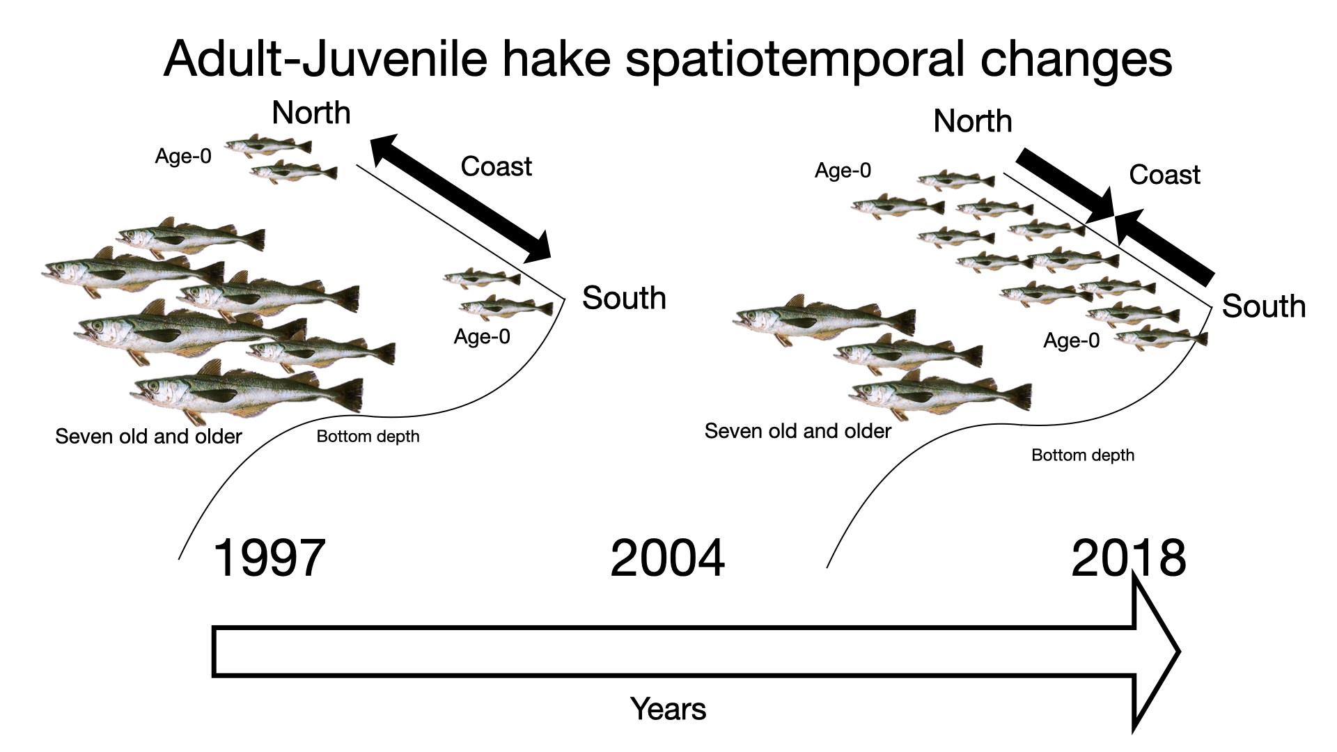
2.1. Study Area and Data

The study area corresponds to the spatial extent of the Chilean hake stock’s assessment cruises, carried out from 1997 to 2018 between 29°39′ S and 42°10′ S every year at the same time (Figure 1). The stock assessment cruises are carried out yearly during the austral winter by a staff member of the Instituto de Fomento Pesquero (IFOP), although no assessment cruises were undertaken in 1998 and 2003 [23]. Although the survey is designed for acoustic estimates of biomass, we utilized logbook data consisting of survey catches and fishing effort, length–frequency data, and length–age keys by sex (Table 1). The code of each research survey allowed us to obtain the database with the grant number allocated by Fondo de Investigación Pesquera y Acuicultura (https://www.subpesca.cl/fipa accessed on 7 April 2022) and IFOP (https://www.ifop.cl accessed on 7 April 2022). IFOP provides information of the swept area (km2) for each fishing haul every year.

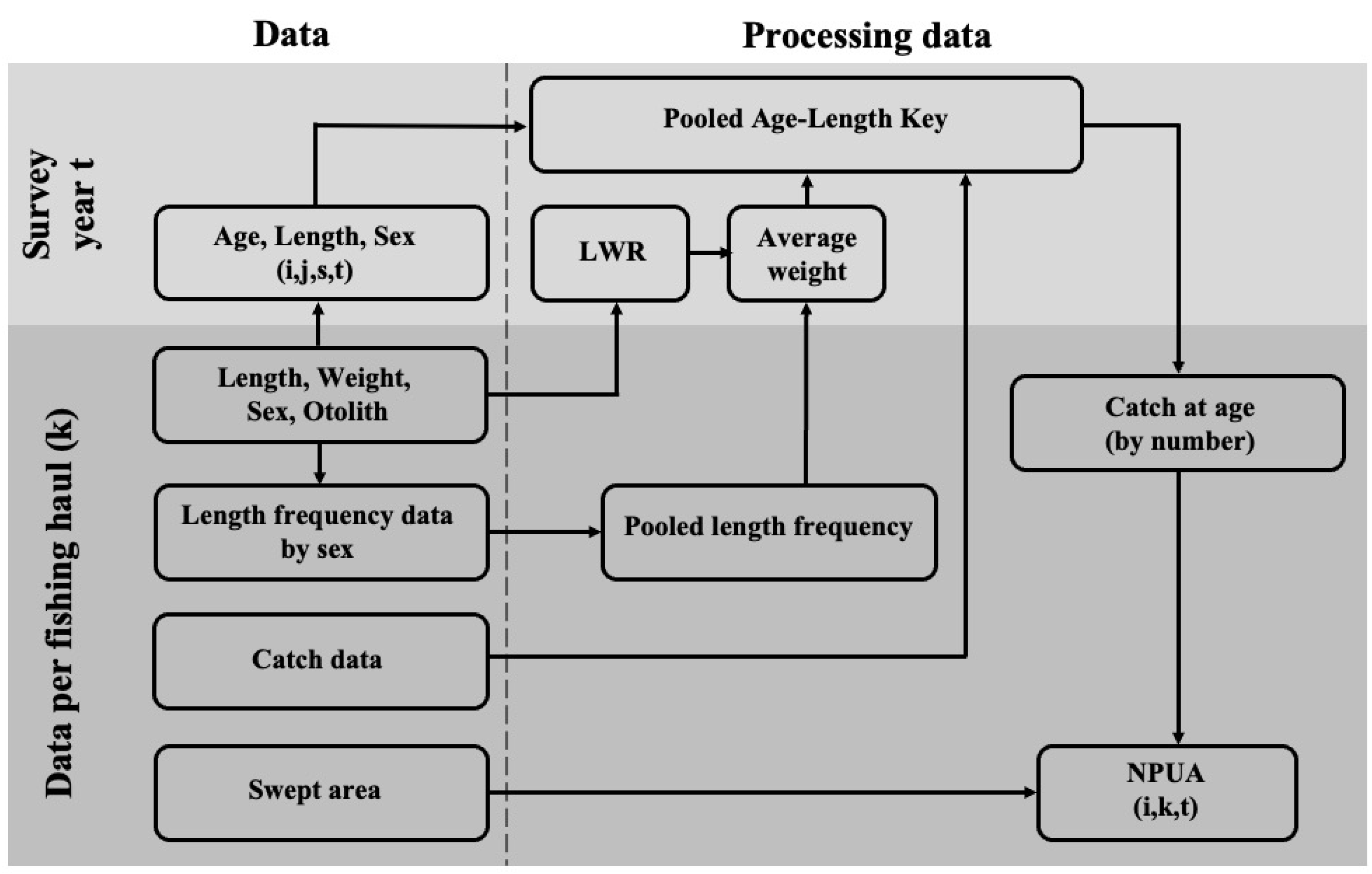
2.2. Age Composition and Abundance per Unit Area

Length–age keys were available by sex for each annual survey and obtained by sampling a fixed number of otoliths. The age composition for each fishing haul was obtained from length–frequency data according to the procedure summarized in Figure 2. Age–length keys (ALK) allowed us to obtain the probability that a fish of age i comes from size j (qi,j); i.e., q i , j = a i , j / j a i , j , where ai,j is the number of individuals with known age i in length class j [33]. For each year and fishing haul, we obtained the number of fish at length class j (fj,k) from length–frequency data per fishing haul (k). The length–frequency data were expanded to the catch (kg) of the fishing haul (Yk) using the average weight, i.e., C j , k = ( Y k / W ¯ k ) f j , k , where C j , k is number caught and W ¯ k is the average weight (kg). Thus, the number of individuals caught by age results from multiplying the number of fish caught at size j (Cj,k) by qi,j, i.e., A i , k = q i , j C j , k , where Ai,k is the number of individuals at the age i in set k. We obtained the number of fish at each age for each fishing haul, which ranged from age 0 to age 14+ (corresponding to fish that were 14 years old or older), and the swept area (km2) allowed us to consider number per unit area (NPUA) as an index of abundance.

2.3. Spatial Distribution and Juvenile–Adult Relationships
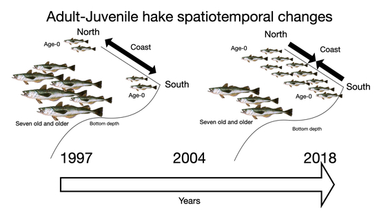
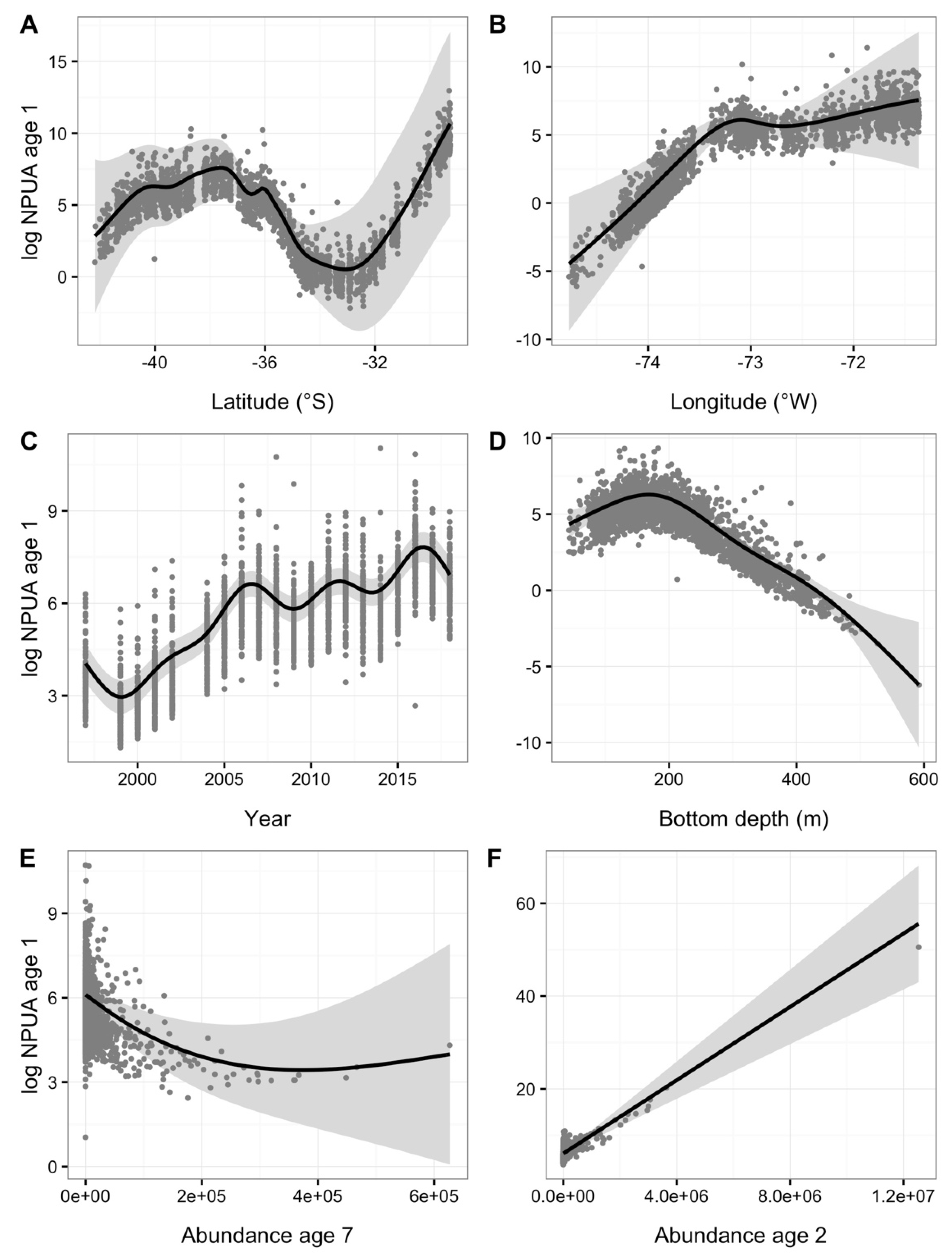
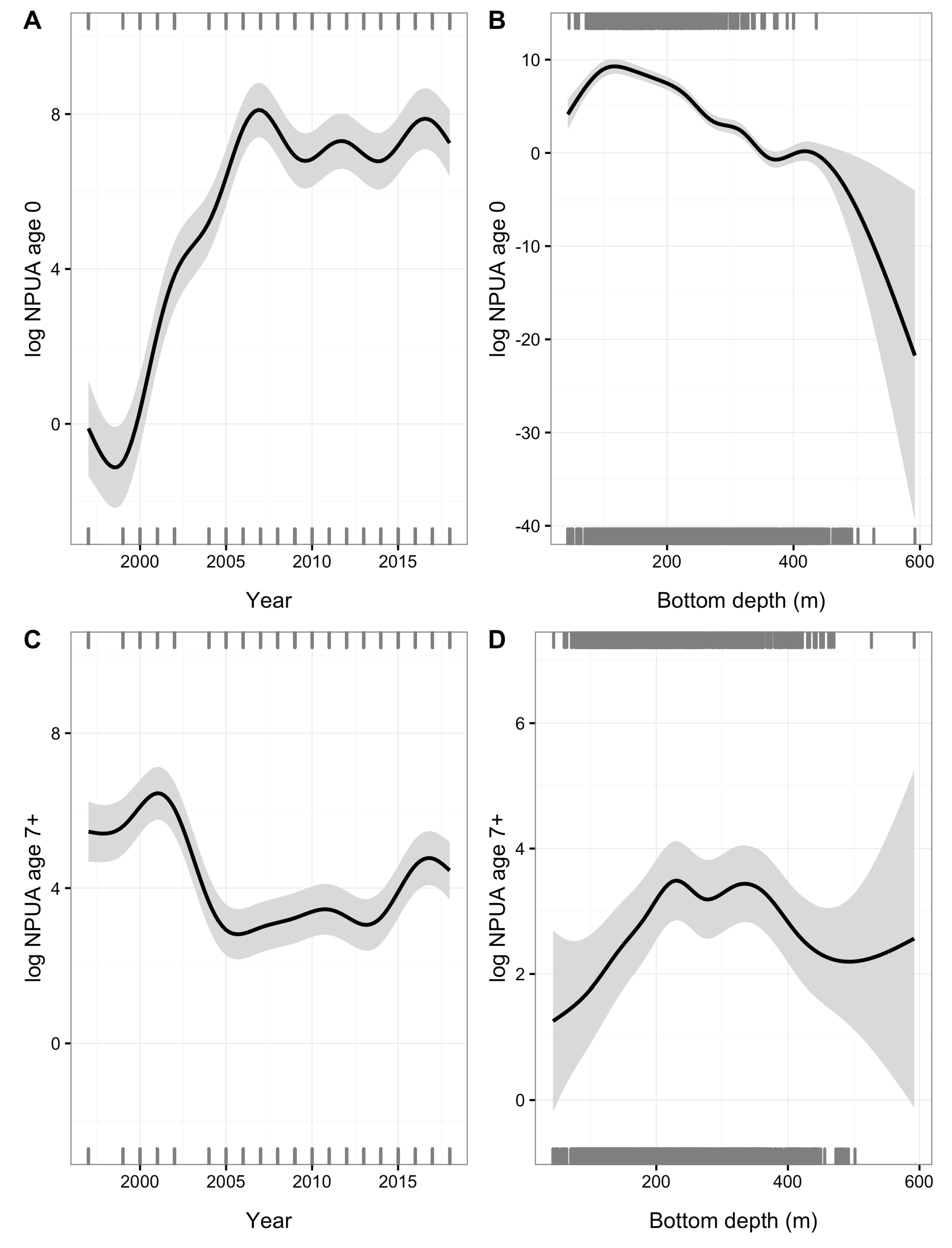
We modeled the spatial distribution of Chilean hake juveniles considering the abundance of age groups 0 and 1 using generalized additive models (GAM), a flexible framework for modeling spatial and temporal effects and the relationship between co-variables through smoother functions [34]. Mainly, we used the “mgcv” package [35] for the statistical software R [36].
Abundance is represented by the NPUA by age groups, whose spatial and temporal distribution often involves a large proportion of zeroes in observations, i.e., zero-inflated data [16,20]. However, the proportion of zeros varied yearly, and the spatial pattern represents several annual realizations observed in each survey, and the sample size defined by the number of hauls was large enough (Table 1). Therefore, we chose a negative binomial distribution to represent the spatiotemporal variable, i.e., Z s , t ~ NB μ s , t , θ , where Z s , t represents the abundance in the spatial locations s = 1, 2, …, S, and temporal index t = 1, 2, …, T, and θ is the dispersion parameter. In GAM, we analyzed the expected number of fish on a log link according to the following expression:
log Z s , t = α + i = 1 I f i X i s , t + log a s , t
where α is the intercept, f i ( ) represents smoother applied to covariables X i s , t , and log a s , t is the logarithm of swept area, without a coefficient to represents the NPUA index; i.e., log n i , t , k = log a i , t , k , where n i , t , k is the number caught of the age group i in year t and fishing haul k, and a i , t , k is the swept area. According to GAM nomenclature, we analyzed spatial and temporal effects separately on the abundance of hake juveniles according to the following linear predictor function:
n i   ~   s t + s x , y , b s = gp , k = 200 + offset ( log a )
where n i is the abundance of either age group 0 or age group 1, and s t is the temporal effects (t = year) considering a smoother spline. s x , y , b s = gp , k = 200 is the smoother spline associated with spatial effects, i.e., the locations of fishing hauls where x and y represent longitude and latitude, respectively. The smoother considered a Gaussian process (bs = gp), based on a Matérn covariance function [34,37], and we set k = 200 as an upper limit on the degree of freedom for smooths. Finally, the offset(log(a)) is the logarithm of swept areas (a) without estimating a coefficient. We omitted subindices for fishing haul and year for better representation of the model.
To investigate significant interactions, we chose a tensor product interaction to detect spatial, temporal, and spatiotemporal effects on the abundance of juveniles. Therefore, we added t i x , y , t , b s = g p , d = c 2 , 1 , k = 200 to the previous model, and we evaluated significant interaction effects applying an analysis of variance (ANOVA) using a chi-squared test. In addition, San Martin et al. [28] found that juveniles tend to be in shallower waters. The abundance and presence, or detection probability, are often related [16,20,38]. Therefore, we added the bottom depth to complete the spatiotemporal distribution modeling of hake juveniles’ abundance, i.e., s d , k = 10 , where d is bottom depth.
Once the spatiotemporal distribution model was completed, we analyzed the endogenous effects through the relationship between juvenile and adult abundance. The average age at maturity was approximately 3.5 years, but since 2004, it has been from around 2.5 to 3 years of age, and hake have begun to reach full maturity by age 5 [25]. Therefore, to avoid the transition from immature to mature individuals in the modeling, we utilized the NPUA of age groups 5, 6, and 7+. The latter is the sum of the abundance of seven-year and older adults. Accordingly, we incorporated the abundance of those age groups into the previous spatiotemporal model sequentially, applying a cubic spline smooth to NPUA of age 5 and 7+, e.g., s n 5 , b s = c s , where n5 is the NPUA of age group 5. In addition, considering that abundance of age 0 and 1 was correlated, we added the NPUA of age 1 to explain the abundance of age 0 juveniles by considering a yearly random effect smoother, i.e., s n 1 , t , b s = r e . Similarly, we incorporated the NPUA of age 2 for modeling juvenile abundance of age 1.
The nomenclature for labeling the model of the relative abundance of age group 0 and age group 1 was M0 and M1, respectively. Models M0.v and M1.v, where v = 1, 2, …, 7, represent models. We compared the models through the explained deviance and log-likelihood and utilized the Akaike Information Criterion (AIC) to select the best model, where A I C = 2 log L + 2 p , log(L) is the maximum value of the likelihood function for the model and p is the number of estimated parameters in the model [39]. In addition, we utilized the difference between AIC ( Δ A I C ) and the relative weight of Δ A I C to compare the performance of the best model, i.e., w m = exp 0.5 Δ A I C m / m = 1 M exp 0.5 Δ A I C m , where m is a given model from all models in the candidate set [40].
Finally, and with comparative purposes, we utilized GAM to describe changes in the abundance of the older adult hake (NPUE 7+). The structure of the model for older adult hake was like the spatiotemporal effect model for age 0 hake, including bottom depth.

3. Results

The abundance of the 0- and 1-year age groups of Chilean hake juveniles had similar patterns of variability, which expresses the positive correlation between these age groups (Figure 3). Likewise, the abundance of juvenile age groups 0 and 1 negatively correlated with the abundance of adults of age groups 5, 6, and 7+. On the other hand, the abundance of adult Chilean hake showed positive correlations, particularly the abundance of age groups 5 and 6, and less with the abundance of older adults (7+).
The spatiotemporal interaction improved the performance of the M0 and M1 models (chi-squared test < 0.01), and the spatial distribution for the abundance of age groups 0 and 1 considering only spatiotemporal effects is summarized through models M0.1 and M1.1, respectively (Table 2). The models M0.1 and M1.1 explained 58.6 and 44.1% of the deviance, respectively. The dispersion parameters of the negative binomial showed low values in agreement with an excess of variability in observations and clumped distribution (Table 2). In addition, the bottom depth significantly improved the spatiotemporal models, increasing the previous deviance explained to 60.8% and 51.8% for models M0.2 and M1.2, respectively (Table 2).
In addition, the endogenous component of the models also showed better explained deviance, especially the effects of the abundance of Chilean hake seven years and older (NPUA 7+) (Table 2). The best endogenous and spatiotemporal model for the abundance of age group 0 juveniles was model M0.7, in which the abundance of age group 1 was also included (Table 2). The deviance explained by model M0.7 was 75.9%. However, note that model M0.8 had a similar performance with an AIC weight of 38.7%. In addition, model M0.8 included the interaction between ages groups 5 and 6, which were correlated (Figure 3). Finally, the best model for the abundance of age one juveniles was model M1.8, including the abundance of age group 2 (Table 2). Model M1.8 explained 95.3% of the deviance with an AIC weight of 99.5%. Those models show that the spatial distribution of hake juveniles varied slightly across years between 1997 and 2018 (Figure 4 and Figure 5).
In these models, and according to partial effects, slight differences in temporal, spatial, and depth effects and negative effects of the abundance of older adults were observed. The abundance of juveniles at age 0 tended to be distributed along the coast with relative maxima between 35 °S and 40°30′ S, peaking at 29 °S, 36 °S a 37°30′ S (Figure 6A). The western distribution tended to decline offshore after 73°30′ W (Figure 6B). The abundance of juveniles of age 0 was located over the continental shelf (<200 m), declining faster after the shelf break (>300 m) (Figure 6D). The temporal effect showed an increment in the abundance from 2002 to 2007, subsequently remaining at high levels (Figure 6E). The endogenous effects show the negative influence of 7-year-old and older adult Chilean hake abundance, and positive effects of age-1 juveniles (Figure 6E,F).
The abundance of age one increased between 36 °S and 40 °S, increasing toward the north of 32 °S (Figure 7A), tended to decline offshore, from 73 °W to 75 °W (Figure 7B), and was located over the continental shelf (<200 m), declining after the shelf break (Figure 7D). The temporal effects showed an increment in abundance after 2000, stabilizing with fluctuations after 2007 and peaking in 2015 (Figure 7C). The endogenous component of the model showed negative effects of older adult hake (7+) (Figure 7E) and positive effects of 2-year-old juvenile hake (Figure 7F).
With a comparative purpose, the spatiotemporal model for the abundance of seven-year-old and older hake was significant (p < 0.01), with an explained deviance of 40%. Thus, the abundance of the younger and older fraction of the stock fluctuated in opposite trends, and the abundance of seven-year-old and older adult hake tended to be distributed at a deeper bottom depth (>200 m) than juveniles of age 0 (Figure 8). Note that there were few data for the depths deeper than 500 m, determining an increase in the confidence limits (Figure 8B,D).

4. Discussion

The relationship between youth and adults in a space–time context indicates population processes associated with endogenous effects on abundance. However, if the juvenile spatial pattern is due to negative interactions with adults, the juvenile abundance may move across the area through time, i.e., changing its spatial distribution [16]. In hake, the spatial distribution of juveniles changed yearly due to changes in abundance rather than in spatial structure. Indeed, the temporal effects showed that the abundance of juvenile hake grew from 2002 to 2007, reaching subsequent stability at higher levels. Thus, juveniles of age 0 and 1 showed similar spatial patterns in abundance, particularly between 35 °S and 40°30′ S and north of 32 °W in shallower depths over the continental shelf, and declining abundance at depths lower than the shelf break. The latitudinal pattern in the younger abundance of hake is coincident with the offshore extension of the continental shelf, which tends to be wide, particularly from 35 °S to 37 °S and from 38 °S to 40 °S [41]. In these areas, the continental shelf and shelf break are bathed by the subsurface Peru–Chile Current flowing towards the pole [42], and the mixing of water masses between the Equatorial Subsurface Water (O2 < 1 mL L−1, 12−13 °C, 35 psu). and the Antarctic Intermediate Water (oxygenated and cold water, 11−12 °C) [43]. Thus, the preference of juvenile hake for shallower waters could be associated with oxygenated waters, but environmental variables contribute little to explain the presence–absence of abundance of Chilean hake [28,29].
Specimens of age 2 were immature individuals before 2004 [25]. However, after 2004, fish of two years reached a proportion of 48% maturity due to the reduction in the maturity length [25,44]. Therefore, immature juveniles of age one began to move towards deeper waters as they grow older [28], explaining the positive correlation of ages 0, 1, and 2, and the negative correlation from age five onwards. Other species of the Merluccius genus show that juveniles prefer to occupy shallow areas [18,45,46], and exhibit an ontogenetic migration from the nurseries to the end of the continental shelf [47,48,49]. Therefore, to minimize the probability of harvesting juvenile age groups during the recruitment process, it is essential to restrict bottom-trawling operations to areas deep enough to consolidate the recruitment process. In Chile, the first five nautical miles of the coast are exclusive to small-scale fishing operations, and industrial bottom trawling is not allowed. In this context, to avoid fishing for age-0 and -1 juvenile recruiting, it is essential to ensure an optimal selection of artisanal spinel and gillnet fishing gear [50,51].
Previous studies showed that juveniles’ presence started in 2004 [22,28]. However, these studies designated fish smaller than 34 cm in length as juveniles. Here, we used abundance by age to study endogenous effects on age- 0 and -1 fish. We know that fish abundance can vary in response to environmental variables [9,52,53,54], migration [18,55,56], and fishing pressure [57,58]. Hake seems to tolerate different environmental conditions due to the wide range of habitats it occupies, from benthic to pelagic through diel migrations [24,28,29,59]. In this context, exogenous factors would not be limiting the distribution of 0- and 1-year-old juveniles, except in the bottom depth and the spatial configuration of the coast, in terms of extension and reduction in the continental shelf and shelf break along the coast. We conclude that the expansion in the abundance of juveniles after 2002 and consolidations after 2007 was favored by the low abundance of older adult hake. However, is important to study the overlap between juveniles and adults in a spatiotemporal context using more rigorous spatiotemporal analysis, such as Bayesian hierarchical models, to identify refuges or nursery areas along the coast [38]. Indeed, generalized additive models (GAM) could only smooth the spatial trend, and autocorrelation in residuals could be approximated by mixed GAM (GAMM) [34]. In part, we used a Gaussian field approach for the smoother spatial term through the covariance function suggested by Kammann and Wand (see details in [35]). Still, the hotspot of juveniles could be identified by hurdle models or by calculating the exceedance probabilities of juvenile abundance being more significant than a given threshold value that is of interest for managers and fishers.
Age-0 and -1 fish could seek refuge in neritic habitats, which would allow them to increase survival by decreasing the risk of predation [31,60], particularly the predation of hake by their ichthyophagous congeners [32]. The negative relationship between the abundance of juveniles at ages 0 and 1 and older adults (7+), shows the potential pressure cannibalism could indirectly exert on younger ages [4,30,31]. These relationships suggest that removing adults by fishing (overexploitation, illegal capture, and discarding) [24,26] could expand the spatial distribution of juveniles in the stock, such as the higher occurrence of juveniles after 2003. These results could contribute to fisheries’ management, recognizing that the juvenile expansion in space–time would help the stock’s sustainability over time. Therefore, it is essential to identify juveniles’ nurseries or recurrent areas outside the fishing grounds and quantify their contribution to the adult stock. The results here are a good starting step to understanding the fundamental factors of the Chilean hake population ecology that are currently not accounted for in stock assessment and management.

Author Contributions

Conceptualization, D.V.Y. and L.A.C.; methodology, L.A.C.; formal analysis, D.V.Y. and L.A.C.; investigation, D.V.Y.; resources, L.A.C.; data curation, D.V.Y.; writing—original draft preparation, D.V.Y.; writing—review and editing, L.A.C. and H.A.; supervision, L.A.C. and H.A.; project administration, L.A.C.; funding acquisition, L.A.C. All authors have read and agreed to the published version of the manuscript.

Funding

This study was funded by Agencia Nacional de Investigación y Desarrollo (ANID) through scholarship ANID-PFCHA/Doctorate National/2017-21170986 to DVY, and LAC was partially funded by Grant COPAS Sur-Austral (ANID PIA APOYO CCTE AFB170006) and COPAS COASTAL (ANID FB210021).

Data Availability Statement

The data that support the findings of this study are available from the corresponding author upon reasonable request.

Acknowledgments

D.V.Y. and L.A.C. thank the “Fondo de Investigación Pesquera y acuicultura” https://www.subpesca.cl/fipa (accessed on 7 April 2022) and Instituto de Fomento Pesquero https://www.ifop.cl (accessed on 7 April 2022) for facilitating the final reports and data associated with the acoustic surveys of Chilean hake.

Conflicts of Interest

The authors declare no conflict of interest.

References

  1. Link, J.S.; Nye, J.A.; Hare, J.A. Guidelines for incorporating fish distribution shifts into a fisheries management context. Fish Fish. 2011, 12, 461–469. [Google Scholar] [CrossRef]
  2. Ward, E.J.; Jannot, J.E.; Lee, Y.-W.; Ono, K.; Shelton, A.O.; Thorson, J.T. Using spatiotemporal species distribution models to identify temporally evolving hotspots of species co-occurrence. Ecol. Appl. 2015, 25, 2198–2209. [Google Scholar] [CrossRef] [PubMed]
  3. Ciannelli, L.; Bailey, K.; Olsen, E.M. Evolutionary and ecological constraints of fish spawning habitats. ICES J. Mar. Sci. 2015, 72, 285–296. [Google Scholar] [CrossRef] [Green Version]
  4. Ohlberger, J.; Rogers, L.A.; Stenseth, N.C. Stochasticity and determinism: How density-independent and density-dependent processes affect population variability. PLoS ONE 2014, 9, 98940. [Google Scholar] [CrossRef] [PubMed] [Green Version]
  5. Ahrens, R.N.M.; Walters, C.J.; Christensen, V. Foraging arena theory. Fish Fish. 2012, 13, 41–59. [Google Scholar] [CrossRef]
  6. Hammerschlag, N.; Heithaus, M.R.; Serafy, J.E. Influence of predation risk and food supply on nocturnal fish foraging distributions along a mangrove-seagrass ecotone. Mar. Ecol. Prog. Ser. 2010, 414, 223–235. [Google Scholar] [CrossRef] [Green Version]
  7. Dalpadado, P.; Bogstad, B.; Eriksen, E.; Rey, L. Distribution and diet of 0-group cod (Gadus morhua) and haddock (Melanogrammus aeglefinus) in the Barents Sea in relation to food availability and temperature. Polar Biol. 2019, 32, 1583–1596. [Google Scholar] [CrossRef]
  8. Nøttestad, L.; Giske, J.; Holst, J.C.; Huse, G. A length-based hypothesis for feeding migrations in pelagic fish. Can. J. Fish. Aquat. Sci. 1999, 56, 26–34. [Google Scholar] [CrossRef]
  9. Eriksen, E.; Ingvaldsen, R.; Stiansen, J.E.; Johansen, G.O. Thermal habitat for 0-group fish in the Barents Sea; how climate variability impacts their density, length, and geographic distribution. ICES J. Mar. Sci. 2012, 69, 870–879. [Google Scholar] [CrossRef]
  10. Thorson, J.T.; Ianelli, J.N.; Kotwicki, S. The relative influence of temperature and size-structure on fish distribution shifts: A case-study on Walleye pollock in the Bering Sea. Fish Fish. 2017, 18, 1073–1084. [Google Scholar] [CrossRef]
  11. Brook, B.W.; Bradshaw, C.J.A. Strength of evidence for density dependence in abundance time series of 1198. Ecology 2006, 87, 1445–1451. [Google Scholar] [PubMed]
  12. Herrando-Pérez, S.; Delean, S.; Brook, B.W.; Bradshaw, C.J.A. Density dependence: An ecological Tower of Babel. Oecologia 2012, 170, 585–603. [Google Scholar] [PubMed]
  13. van Gemert, R.; Andersen, K.H. Challenges to fisheries advice and management due to stock recovery. ICES J. Mar. Sci. 2018, 75, 1864–1870. [Google Scholar]
  14. Andersen, K.H.; Jacobsen, N.S.; Jansen, T.; Beyer, J.E. When in life does density dependence occur in fish populations? Fish Fish. 2017, 18, 656–667. [Google Scholar]
  15. Lorenzen, K.; Camp, E.V. Density-dependence in the life history of fishes: When is a fish recruited? Fish. Res. 2019, 217, 5–10. [Google Scholar]
  16. Morfin, M.; Fromentin, J.-M.; Jadaud, A.; Bez, N. Spatio-temporal patterns of key exploited marine species in the Northwestern Mediterranean sea. PLoS ONE 2012, 7, e37907. [Google Scholar]
  17. Bartolino, V.; Ottavi, A.; Colloca, F.; Ardizzone, G.D.; Stefánsson, G. Bathymetric preferences of juvenile European hake (Merluccius merluccius). ICES J. Mar. Sci. 2008, 65, 963–969. [Google Scholar]
  18. Jansen, T.; Kristensen, K.; Kainge, P.; Durholtz, D.; Strømme, T.; Thygesen, U.H.; Wilhelm, M.R.; Kathena, J.; Fairweather, T.P.; Paulus, S.; et al. Migration, distribution and population (stock) structure of shallow-water hake (Merluccius capensis) in the Benguela Current Large Marine Ecosystem inferred using a geostatistical population model. Fish Res. 2016, 179, 156–167. [Google Scholar]
  19. Tamdrari, H.; Castonguay, M.; Brêthes, J.C.; Duplisea, D. Density-independent and -dependent habitat selection of Atlantic cod (Gadus morhua) based on geostatistical aggregation curves in the northern Gulf of St Lawrence. ICES J. Mar. Sci. 2010, 67, 1676–1686. [Google Scholar]
  20. Izquierdo, F.; Paradinas, I.; Cerviño, S.; Conesa, D.; Alonso-Fernández, A.; Velasco, F.; Preciado, I.; Punzón, A.; Saborido-Rey, F.; Pennino, M.G. Spatio-temporal assessment of the European hake (Merluccius merluccius) Recruits in the Northern Iberian Peninsula. Frontiers Mar. Sci. 2021, 8, 614675. [Google Scholar]
  21. Aguayo-Hernández, M. Biology and fisheries of Chilean hakes (M. gayi and M. australis). In Hake: Biology, Fisheries and Markets; Alheit, J., Pitcher, T.J., Eds.; Springer: Dordrecht, The Netherlands, 1995; pp. 305–337. [Google Scholar]
  22. Evaluación Directa De Merluza Común. 2016. Instituto de Fomento Pesquero, Valparaíso. Available online: https://www.ifop.cl (accessed on 22 February 2022).
  23. Evaluación Directa De Merluza Común. 2018. Instituto de Fomento Pesquero, Valparaíso. Available online: https://www.ifop.cl (accessed on 22 February 2022).
  24. Gatica, C.; Neira, S.; Arancibia, H.; Vásquez, S. The biology, fishery and market of Chilean hake (Merluccius gayi gayi) in the Southeastern Pacific Ocean. In Hakes; Arancibia, H., Ed.; Wiley-Blackwell: Hoboken, NJ, USA, 2015; pp. 126–153. [Google Scholar]
  25. Instituto de Fomento Pesquero. Estatus Y Posibilidades De Explotación Biológicamente Sustentables De Los Principales Recursos Pesqueros Nacionales, Año 2018: Merluza común; Instituto de Fomento Pesquero: Valparaíso, Chile, 2018. [Google Scholar]
  26. Arancibia, H.; Neira, S. Overview of the Chilean hake (Merluccius gayi) stock. A biomass forecast, and the jumbo squid (Dosidicus gigas) predator-prey relationship off Central Chile (33 °S– 39°S). CalCOFI Rep. 2008, 49, 104–115. [Google Scholar]
  27. Alarcón-Muñoz, R.; Cubillos, L.; Gatica, C. Jumbo squid (Dosidicus gigas) biomass off central Chile: Effects on chilean hake (Merluccius gayi). CalCOFI Rep. 2008, 49, 157–166. [Google Scholar]
  28. San Martín, M.A.; Cubillos, L.A.; Saavedra, J.C. The spatio-temporal distribution of juvenile hake (Merluccius gayi gayi) off central southern Chile (1997–2006). Aquat. Living Resour. 2011, 24, 161–168. [Google Scholar] [CrossRef] [Green Version]
  29. San Martín, M.A.; Wiff, R.; Saavedra-Nievas, J.C.; Cubillos, L.A.; Lillo, S. Relationship between Chilean hake (Merluccius gayi gayi) abundance and environmental conditions in the central-southern zone of Chile. Fish. Res. 2013, 143, 89–97. [Google Scholar] [CrossRef]
  30. Cubillos, L.A.; Alarcón, C.; Arancibia, H. Selectividad por tamaño de las presas en merluza común (Merluccius gayi gayi), zona centro-sur de Chile (1992–1997). Investig. Mar. 2007, 35, 55–69. [Google Scholar] [CrossRef]
  31. Link, J.S.; Lucey, S.M.; Melgey, J.H. Examining cannibalism in relation to recruitment of silver hake Merluccius bilinearis in the U.S. northwest Atlantic. Fish. Res. 2012, 114, 31–41. [Google Scholar] [CrossRef]
  32. Jurado-Molina, J.; Gatica, C.; Cubillos, L.A. Incorporating cannibalism into an age-structured model for the Chilean hake. Fish. Res. 2006, 82, 30–40. [Google Scholar] [CrossRef]
  33. Kimura, D.K. Statistical Assessment of the Age–Length Key. J. Fish. Board Can. 1977, 34, 317–324. [Google Scholar] [CrossRef]
  34. Wood, S. Generalized Additive Models: An Introduction with R, 2nd ed.; CRC/Taylor & Francis: New York, NY, USA, 2017. [Google Scholar]
  35. Cran. Available online: https://cran.r-project.org/web/packages/mgcv/index.html (accessed on 22 February 2022).
  36. R-project. Available online: https://www.R-project.org/ (accessed on 22 February 2022).
  37. Simpson, G.L. Modelling palaeoecological time series using Generalised Additive Models. Frontiers Ecol. Evol. 2018, 6, 149. [Google Scholar] [CrossRef] [Green Version]
  38. Paradinas, I.; Conesa, D.; López-Quílez, A.; Bellido, J.M. Spatio-temporal model structures with shared components for semi-continuous species distribution modelling. Spat. Stat. 2017, 22, 434–450. [Google Scholar] [CrossRef]
  39. Akaike, H. A new look at the statistical model identification. IEEE T. Automat. Contr. 1974, 19, 716–723. [Google Scholar] [CrossRef]
  40. Buckland, S.T.; Burnham, K.P.; Augustin, N.H. Model selection: An integral part of inference. Biometrics 1997, 53, 603–618. [Google Scholar] [CrossRef]
  41. Sobarzo, M.; Bravo, L.; Donoso, D.; Garcés-Vargas, J.; Schneider, W. Coastal upwelling and seasonal cycles that influence the water column over the continental shelf off central Chile. Prog. Oceanogr. 2007, 75, 363–382. [Google Scholar] [CrossRef]
  42. Contreras, M.; Pizarro, O.; Dewitte, B.; Sepulveda, H.H.; Renault, L. Subsurface mesoscale eddy generation in the ocean off Central Chile. J. Geophys. Res. Oceans 2019, 124, 5700–5722. [Google Scholar] [CrossRef] [Green Version]
  43. Silva, N.; Neshyba, S. On the Southernmost Extension of the Peru-chile Undercurrent. Deep-Sea Res. Part I Oceanogr. Res. Pap. 1979, 26, 1387–1393. [Google Scholar]
  44. Biología Reproductiva de Merluza Común. FIPA 2006-16. Available online: https://www.subpesca.cl/fipa/613/w3-article-89139.html (accessed on 22 February 2022).
  45. Cantafaro, A.; Ardizzone, G.; Enea, M.; Ligas, A.; Colloca, F. Assessing the importance of nursery areas of European hake (Merluccius merluccius) using a body condition index. Ecol. Ind. 2017, 81, 383–389. [Google Scholar] [CrossRef]
  46. Carlucci, R.; Giuseppe, L.; Porzia, M.; Francesca, C.; Alessandra, M.C.; Letizia, S.; Teresa, S.M.; Nicola, U.; Angelo, T.; D’Onghia, G. Nursery areas of red mullet (Mullus barbatus), hake (Merluccius merluccius) and deep-water rose shrimp (Parapenaeus longirostris) in the Eastern-Central Mediterranean Sea. Estuar. Coast. Shelf Sci. 2009, 83, 529–538. [Google Scholar] [CrossRef]
  47. Abella, A.; Serena, F.; Ria, M. Distributional response to variations in abundance over spatial and temporal scales for juveniles of European hake (Merluccius merluccius) in the Western Mediterranean Sea. Fish. Res. 2005, 71, 295–310. [Google Scholar] [CrossRef]
  48. Fiorentino, F.; Garofalo, G.; Santi, A.D.; Bono, G.; Giusto, G.B.; Norrito, G. Spatio-Temporal distribution of recruits (0 group) of Merluccius merluccius and Phycis blennoides (Pisces, Gadiformes) in the Strait of Sicily (Central Mediterranean). In Migrations and Dispersal of Marine Organisms; Developments in Hydrobiology; Jones, M.B., Ingólfsson, A., Ólafsson, E., Helgason, G.V., Gunnarsson, K., Svavarsson, J., Eds.; Springer: Dordrecht, The Netherlands, 2003; Volume 174, pp. 223–236. [Google Scholar]
  49. Maynou, F.; Lleonart, J.; Cartes, J.E. Seasonal and spatial variability of hake (Merluccius merluccius L.) recruitment in the NW Mediterranean. Fish. Res. 2003, 60, 65–78. [Google Scholar] [CrossRef]
  50. Queirolo, D.; Gaete, E.; Ahumada, M. Gillnet selectivity for Chilean hake (Merluccius gayi gayi Guichenot, 1848) in the bay of Valparaíso. J. Appl. Ichthyol. 2013, 29, 775–781. [Google Scholar] [CrossRef]
  51. Queirolo, D.; Flores, A. Seasonal variability of gillnet selectivity in Chilean hake Merluccius gayi gayi (Guichenot, 1848). J. Appl. Ichthyol. 2017, 33, 699–708. [Google Scholar] [CrossRef]
  52. Capuzzo, E.; Lynam, C.P.; Barry, J.; Stephens, D.; Forster, R.M.; Greenwood, N.; McQuatters-Gollop, A.; Silva, T.; van Leeuwen, S.M.; Engelhard, G.H. A decline in primary production in the North Sea over 25 years, associated with reductions in zooplankton abundance and fish stock recruitment. Glob. Change Biol. 2018, 24, e352–e364. [Google Scholar] [CrossRef] [PubMed]
  53. Malick, M.; Hunsicker, M.; Haltuch, M.; Parker-Stetter, S.; Berger, A.; Marshall, K. Relationships between temperature and Pacific hake distribution vary across latitude and life-history stage. Mar. Ecol. Progr. Ser. 2020, 639, 185–197. [Google Scholar] [CrossRef]
  54. Thiaw, M.; Auger, P.A.; Ngom, F.; Brochier, T.; Faye, S.; Diankha, O.; Brehmer, P. Effect of environmental conditions on the seasonal and inter-annual variability of small pelagic fish abundance off North-West Africa: The case of both Senegalese sardinella. Fish. Oceanogr. 2017, 26, 583–601. [Google Scholar] [CrossRef]
  55. Kathena, J.N.; Yemane, D.; Bahamon, N.; Jansen, T. Population abundance and seasonal migration patterns indicated by commercial catch-per-unit-effort of hakes (Merluccius capensis and M. paradoxus) in the northern Benguela Current Large Marine Ecosystem. Afr. J. Mar. Sci. 2018, 40, 197–209. [Google Scholar] [CrossRef] [Green Version]
  56. Vine, J.R.; Kanno, Y.; Holbrook, S.C.; Post, W.C.; Peoples, B.K. Using side-scan sonar and n-mixture modeling to estimate Atlantic sturgeon spawning migration abundance. N. Am. J. Fish. Manag. 2019, 39, 939–950. [Google Scholar] [CrossRef]
  57. Camara, M.L.; Mérigot, B.; Leprieur, F.; Tomasini, J.A.; Diallo, I.; Diallo, M.; Jouffre, D. Structure and dynamics of demersal fish assemblages over three decades (1985–2012) of increasing fishing pressure in Guinea. Afr. J. Mar. Sci. 2016, 38, 189–206. [Google Scholar] [CrossRef]
  58. Kuparinen, A.; Boit, A.; Valdovinos, F.S.; Lassaux, H.; Martinez, N.D. Fishing-induced life-history changes degrade and destabilize harvested ecosystems. Sci. Rep. 2016, 6, 22245. [Google Scholar] [CrossRef] [Green Version]
  59. Ponce, T.; Cubillos, L.A.; Ciancio, J.; Castro, L.R.; Araya, M. Isotopic niche and niche overlap in benthic crustacean and demersal fish associated to the bottom trawl fishing in south-central Chile. J. Sea Res. 2021, 173, 102059. [Google Scholar] [CrossRef]
  60. Olsson, K.H.; Andersen, K.H. Cannibalism as a selective force on offspring size in fish. Oikos 2018, 127, 1264–1271. [Google Scholar] [CrossRef] [Green Version]
Figure 1. Study area shown in the square in Chile (left) and distribution of the fishing hauls (right) obtained during the Chilean hake stock assessment survey in the period between 1997 and 2018.
Fishes 07 00088 g001
Figure 2. Survey data processing flow to obtain catch-at-age data, and hence an abundance index per age group i, fishing hauls k, and year t. Age (i), length (j), and sex (s) from fishing hauls allowed us to obtain a pooled age–length key (both sexes) for survey t, which was utilized to obtain catch at age from pooled length–frequency (both sexes). The abundance index is catch in number per unit of area, where the area is the swept area of each haul.
Fishes 07 00088 g002
Figure 3. Coefficients of Spearman correlation obtained between the abundance index per age groups of Chilean hake, where n0, n1, …, n7+ represent the NPUA (individuals per km2) of age groups 0, 1, 2, …, 7 and older.
Fishes 07 00088 g003
Figure 4. Spatiotemporal distribution of the abundance of Chilean hake juvenile of age 0, from 1997 to 2018 (Model M0.7, Table 2).
Fishes 07 00088 g004
Figure 5. Spatiotemporal distribution of the abundance of Chilean hake juvenile of age 1, from 1997 to 2018 (Model M1.8, Table 2).
Fishes 07 00088 g005
Figure 6. Relationships between the abundance of juvenile Chilean hake of age 0 and relevant variables for spatiotemporal effects latitude (A), longitude (B), year (C), bottom depth (D) and endogenous effects of older adult hake of age 7+ (E) and juvenile hake of age-1 (F), according to the best model fitted (Model M0.7, Table 2).
Fishes 07 00088 g006
Figure 7. Relationships between the abundance of juvenile Chilean hake of age 1 and relevant variables for spatiotemporal effects of latitude (A), longitude (B), year (C), bottom depth (D), and endogenous effects of older adult hake of age 7+ (E) and juvenile hake of age-2 (F), according to the best model fitted (Model M1.8, Table 2).
Fishes 07 00088 g007
Figure 8. Temporal changes in log abundance and distribution of the abundance as a function of the bottom depth: log abundance of age 0 (A,B), and log abundance of age 7+ (C,D).
Fishes 07 00088 g008
Table 1. Year, survey code, and number of specimens and fishing tows utilized to build the database. Code = grant number of the survey. ALK = age–length key, where n is the number of specimens (=otoliths) utilized to build the ALK for each year. WLD = weight–length data, where n is the total number of specimens utilized to obtain length–weight relationships, and hence the mean weight of length classes. LFD = length–frequency data, where n is the total number of specimens sampled in each year. Tows = number of trawls, where n is the number per year. Source: technical reports available in https://www.subpesca.cl/fipa/ (accessed on 7 April 2022) and https://www.ifop.cl (accessed on 7 April 2022).
YearCodeALK (n)WLD (n)LFD (n)Tows (n)
19971997-12972375423,497133
19991999-04999369915,035135
20002000-041011221621,952124
20012001-181045269326,427141
20022002-031138377829,210153
20042004-091013362417,570137
20052005-05726332116,516138
20062006-031117359917,819134
20072007-16997466928,080171
20082008-14993424026,648153
20092009-13572433516,673149
20102010-10544322612,102125
20112011-03647380012,310138
20122012-04659364811,375138
20132013-12635367913,645146
2014682-020627338713,397136
2015682-03262129959419104
2016682-042653415513,914145
2017682-046644354811,947127
2018682-056625381311,935135
Table 2. Models evaluated to explain the number of Chilean hake juveniles of age groups 0 (n0) and 1 (n1), during the austral winter, between 1997 and 2018. The GAM model considered the negative binomial distribution and link log. The number of age 7 (n7) is the number per unit area of 7-year-old and older adult hake. The nomenclature is t = year, x = longitude, y = latitude, a = swept area, and d = bottom depth. The GAM smother terms are explained in the text, and NB(θ) is the estimated dispersion parameter of negative binomial distribution. The selected model is M07 and M1.8 according to the Akaike’s Information Criterion (AIC).
ModelLinear PredictorNB(θ)Deviance ExplainedLog-LikelihoodAICΔAICAIC Weight
M0 n 0   ~   s t + s x , y , b s = gp , k = 200 + offset ( log a ) 0.13855.5−9675.918,961.87572.290.0
M0.1 M 0 + t i x , y , t , b s = gp , d = c 2 , 1 , k = 200 0.14758.6−9645.518,874.29484.710.0
M0.2 M 0 . 1 + s d , k = 10 0.16060.8−9392.118,606.05216.470.0
M0.3 M 0 . 2 + s n 5 , b s = c s 0.16361.5−9386.818,584.78195.200.0
M0.4 M 0 . 3 + s n 1 , t , b s = r e 0.17976.7−9333.418,420.2430.660.0
M0.5 M 0 . 2 + s n 1 , t , b s = r e + s n 5 , n 6 0.17975.6−9327.518,418.5328.950.0
M0.6 M 0 . 2 + s n 7 , b s = c s 0.16461.9−9381.018,571.10181.520.0
M0.7 M 0 . 6 + s n 1 , t , b s = r e 0.18175.9−9315.818,389.580.0061.3
M0.8 M 0 . 7 + s n 5 , n 6 0.18276.8−9314.518,390.500.9238.7
M1 n 1   ~   s t + s x , y , b s = gp , k = 200 + offset ( log a ) 0.23040.5−13,664.026,955.161333.840.0
M1.1 M 1 + t i x , y , t , b s = gp , d = c 2 , 1 , k = 200 0.24444.1−13,619.026,822.371201.050.0
M1.2 M 1 . 1 + s d , k = 10 0.28851.8−13,242.026,256.11634.790.0
M1.3 M 1 . 2 + s n 5 , b s = c s 0.29552.9−13,227.026,198.38577.060.0
M1.4 M 1 . 3 + s n 2 , t , b s = r e 0.36595.1−12,936.025,641.2519.930.0
M1.5 M 1 . 2 + s n 2 , t , b s = r e + s n 5 , n 6 0.36895.3−12,932.025,631.7210.400.5
M1.6 M 1 . 2 + s n 7 , b s = c s 0.28952.0−13,240.026,251.62630.300.0
M1.7 M 1 . 6 + s n 2 , t , b s = r e 0.36595.1−12,938.025,644.3323.010.0
M1.8 M 1 . 7 + s n 5 , n 6 0.36995.3−12,926.025,621.320.0099.5
Publisher’s Note: MDPI stays neutral with regard to jurisdictional claims in published maps and institutional affiliations.

