Article

From Transient to Sedentary? Changes in the Home Range Size and Environmental Patterns of Movements of European Eels (Anguilla anguilla) in a Mediterranean River

by
Mercedes Herrera
*,
Raquel Moreno-Valcárcel
,
Ramón De Miguel Rubio
and
Carlos Fernández-Delgado
Departamento de Zoología, Universidad de Córdoba, Edificio Charles Darwin, Campus de Rabanales, 14071 Córdoba, Spain
*
Author to whom correspondence should be addressed.
Fishes 2019, 4(3), 43; https://doi.org/10.3390/fishes4030043
Submission received: 29 March 2019 / Revised: 6 August 2019 / Accepted: 7 August 2019 / Published: 13 August 2019

Abstract

:
The habitat use of eels during the development of sedentary behavior, which depends on the animals’ body size, is unknown. Our objective was to analyze, for two years, the changes in the home range of a population of European eel (Anguilla anguilla, Linnaeus, 1758) in Southern Europe in relation to the animals’ body length (TL), and the influence of environmental factors (water temperature and flow) on the local movements of this population through observation of their sedentary behavior. We used a previously-validated mark–recapture methodology, obtaining a low deviation in the estimation of the extension of the eels’ movements. Our results revealed relatively short movements in relation to other populations, and we hypothesize that this could be related to the high habitat diversity and low eel population density in the study area. The home range size showed a high variability and dispersion among the smallest eels, however, as TL increased, the variability of home range size decreased, and home ranges were larger. These changes could be associated with the acquisition of a sedentary lifestyle. Once eels had become sedentary, an environmental pattern was observed between their movements and the water temperature and flow, with larger movements observed as the flow increased and water temperature decreased. This suggests that the temporal and spatial scales of observation are of crucial importance for monitoring eel populations and for the study of population size structure, population dynamics, and biology, which can be used to improve conservation strategies.

1. Introduction

The population of the European eel (Anguilla anguilla, Linnaeus, 1758) started to decline in the 1980s. This was accompanied by a decrease in the continental stock, to such a degree that the International Council for the Exploration of the Sea–European Inland Fisheries Advisory Commission (ICES-EIFAC) Working Group on Eels (WGEEL) concluded that the species was outside the safe biological limits [1]. This situation led the European Commission to create a regulation (EC 1100/2007) requiring European member states to develop eel management plans, with the aim of reaching 40% of pristine escapement to the sea. According to the ICES [1,2,3], the effectiveness of this plan largely depends on information about the distinctive features of the eel life cycle for subpopulations in the species’ entire distribution area.
The study of the movements is relevant from a basic and applied scientific perspective [4,5,6,7]. It allows habitat use to be determined, which is essential to understanding subpopulation size structure and the behavioral ecology of eels; these in turn are fundamental parameters for the construction of effective management plans directed at the conservation of the species [8,9,10,11,12,13]. Additionally, the understanding of eel movements is critical for estimating true density by calculating the Effective Sampling Area [14] and also for defining spatial limits for an operational sampling strategy for monitoring eel populations [15,16].
The present study has two focuses. Firstly, it focuses on one of the areas where the life history traits of the European eel are less well known—the southern Iberian Peninsula. Movements of eel populations have been studied in different areas and habitats [11,13,16,17,18,19]. It is widely known that large environments, such as estuaries or river–estuary interfaces, promote large movements of eels [10,12,13,16,20]. In rivers, it has been reported that the extension of eel movements is determined by biotic or abiotic factors, such as river typology or food availability [11,17]. In the Iberian Peninsula, there has only been one study addressing eel movements, in a small lake [21], and the use of space and the movements of European eels in rivers in this area are, therefore, still unknown. It is well known that water temperature has a strong influence on the activity of eels; they show little or no activity during months in which the temperature drops below 10–12 °C and show peaks of activity in summer [15,17,19,22]. These patterns correspond to the temperature cycle of the northern latitudes. However, in the southern zone of the distribution of the European eel, which includes the Mediterranean area, temperatures rarely fall below 10 °C. Therefore, if there is an environmental pattern in the movements of eels in the Guadiaro River, Southern Spain—the area investigated in the present study—it would be expected to be different from the patterns at more northerly latitudes.
The upstream migrations and large-scale movements of eels in inland waters are well understood [8], as is the relationship between body size and the process of acquiring sedentary behavior [9]. However, the evolution of the home range size of eels and the possible existence of different environmental patterns of local movements in relation to both body length and the acquisition of sedentary behavior have never been studied. Therefore, these are the second focus of this study.
Compared with the use of telemetry, the study of the movements using mark–recapture techniques allows data to be obtained for a large number of individuals, even for small-sized animals, with limited research budgets [23]. It also allows long-term monitoring, which is of vital importance for the study of the home range size, since calculations performed for periods of less than one year may not include seasonal variations and may thus produce less accurate estimates [24]. The main disadvantage of mark–recapture techniques comes from the interpretation of the obtained results, since the recapture rates generally decrease as the distance the animal moves increases [25,26]. This problem, known as distance-weighted sampling [14], biases the estimation of distance distributions [23]. Traditionally, it has been considered that the movements of fish follow the general rule of what has been called the Restricted Movement Paradigm (RMP) [27,28,29]. According to the RMP, most individuals are relatively nonmobile and restrict their movements to a well-defined home range, with observed movements showing a leptokurtic distribution [7,30]. However, RMP has been increasingly criticized, since it has been considered as being a consequence of the bias of distance-weighted sampling [28] or of heterogeneity in the movement patterns within a population composed of stationary and mobile groups [7,30,31]. In any case, the use of mark–recapture methods introduces the possibility of bias in the probability of detection of long movements of animals, which must be evaluated.
The objectives of this study were to test and quantify the bias due to the mark–recapture methodology; to determine the extent of local movements of eels, the eels’ home ranges in relation to body size (>25 cm Total Length, TL) throughout the process of acquiring sedentary behavior, and, finally, the possible environmental factors that influence local movements. The study was carried out on an eel population located in the middle reaches of the Guadiaro River, in the southernmost part of the European distribution area of the European eel, for a period of two years.

2. Results

2.1. Effects of Passive Integrated Transponder Tags and Tag Retention

A total of 182 eels were used to test the effects of Passive Integrated Transponder (PIT) tags and tag retention. Of these, only two died during the study period—one marked with a PIT with a size of 8.0 × 2.1 mm and one unmarked eel. This implies a mortality rate of 1.1% for the total study group and of 1% for the tagged eels. The retention rate for nine months was 100%.
Increase in body mass was found to be correlated to the time elapsed from the beginning of the experiment (T, days) (covariance analysis, F = 44.55; p < 0.001) and TL (F = 7743.05; p < 0.001), and the interaction between T and TL was significant (F = 2.78; p = 0). In contrast, there were no significant differences in the increase in body mass between eels with and without PIT (F = 0.04; p = 0.96), or in the interactions in which this variable was present.
A two-way ANOVA showed significant differences in the response variable, namely the Residual Condition Index (Kr), over the time elapsed from the beginning of the experiment (F = 76.54; p = 0). However, there were no significant differences in Kr between marked and unmarked specimens (F = 0.005; p > 0.05).

2.2. Movements and Home Range

Data were obtained from 296 eels recaptured at least once. It was found that the Distance between Captures (DC or observed movements) was independent of the Number of Days (D) (F = 0.295; p = 0.590; R2 = 0.001), and, therefore, all of the 296 specimens were used in subsequent analyses. TL ranged from 25.0 to 68.3 cm ( X ¯ T L = 32.4 ± 0.41 cm at the 95% confidence interval (C.I.)). A total of 127 specimens (mean X ¯ T L = 34.0 ± 0.59 cm at the 95% C.I.) were recaptured two or more times. The maximum number of recaptures (n = 12) was made for two individuals with TLs of 37.3 cm and 42.9 cm. All studied eels were in the FI to FIII maturation stages [32].

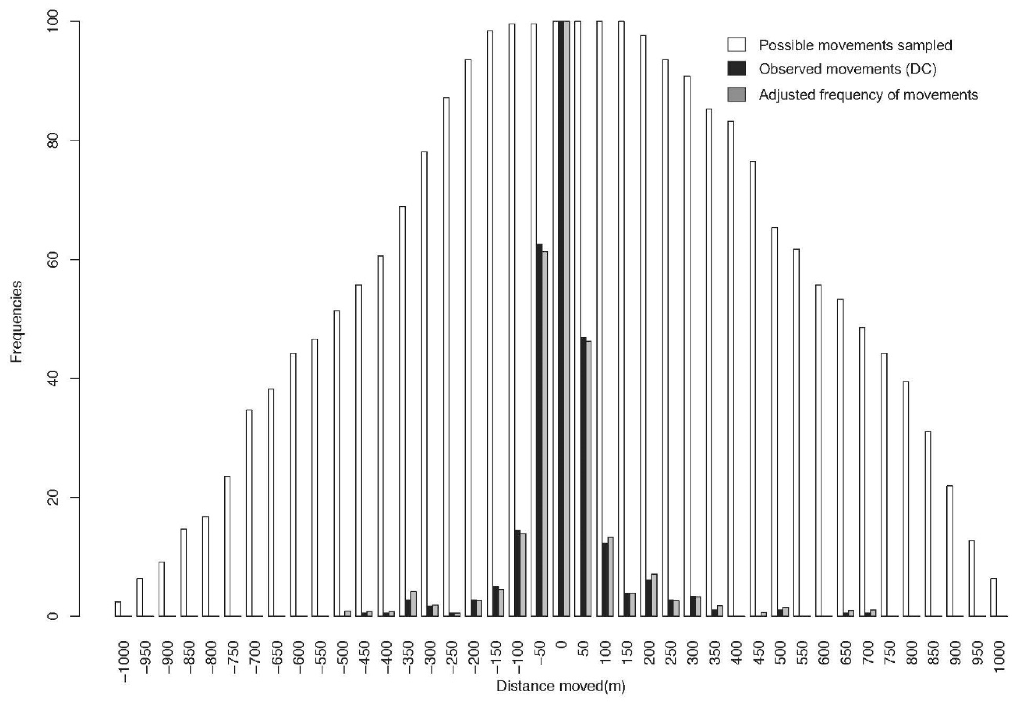
2.2.1. Deviation Estimate of Observed Movements

Given the extension of eel movement, the probability of the detection of eel movement was not homogeneous over all the distances sampled (white bars in Figure 1). This implies that there was bias in the estimates of the extension of movements due to the distance-weighted sampling phenomenon, and that it increases as the distance from the sample location to the original point of release increases. There were no significant differences between the observed movements and those obtained theoretically (Mann–Whitney test; U = 138,182.50; p = 0.928); however, there was an evident difference in kurtosis, with significant differences observed in the comparison of the respective mean (observed movements-possible movements sampled) positive and negative values (negative: U = 10,518.00; p = 0.000; positive: U = 10,692.50; p = 0.000). Thus, the null hypothesis that the distribution of DC (observed movements) was random could be rejected. Therefore, accepting that each possible distance moved (DC) (from 0 to ± 1000 m; white bars in Figure 1; theoretical distribution) should be observed, it can be concluded that the real DCs (black bars in Figure 1) had a smaller extension than possible movements detected with a probability greater than 0.
Consequently, despite the above-mentioned distance-weighted sampling phenomenon, 90% of the DCs observed, which were between the 5th (−164.80 m) and 95th (+174.07 m) percentiles (corresponding to −200 m and +200 m in the frequency distribution of the theoretical probabilities measured at intervals of 50 m, Figure 1), had a higher average detection probability (98.76 ± 1.62%), since they were located in the area of the theoretical distribution with high detection probabilities. The remaining 10% of the DCs observed were detected with an average probability of 69.38% ± 8.1%. The most extreme movements recorded, namely −450 m and +750 m, which had individual frequencies lower than 1%, had theoretical detection probabilities of 55.78% and 48.61%, respectively.
After applying the Correction Factor, there were no significant differences between the frequency distributions of the DCs and the corrected DCs (U = 845.00; p = 0.729) or between the positive (U = 283.50; p = 0.730) or negative DCs-corrected DCs (U = 197.50; p = 0.678). The adjustment had no effect on movements between −250 and +300 m (representing more than 90% of the detected movements), and only slightly affected the most extreme movements (Figure 1).

2.2.2. Distance between Captures (DC, Observed Movements)

The frequency distribution of the DCs was found to be symmetrical (z = 1.349; p > 0.05) (Figure 1), which implies an absence of directionality in the eel movements. Therefore, the absolute values of the extension of the movements were used. More than 60% of the total movements (n = 558) were less than 50 m (Figure 2a), with a mean value of 64.27 ± 7.78 m at the 95% C.I.
The distribution of DC was significantly asymmetric (z = 19.02; p < 0.001) and leptokurtic (z = 29.91; p < 0.001) with a high degree of dispersion (Figure 2a). The standard deviation was 93.55 m, the range was 581 m, and outliers and extreme values were up 158.70 m.
The Movement Rate (MR) of the eels was 34.59%. With increasing length (TL), individuals became more mobile, with a progressive increment in MR being observed as their length increased. In the TL range of 25.0–29.9 cm, MR was 26.88%; in the range 30.0–34.9 cm, MR was 32.10%; and for TLs > 50 cm, MR was 64.29%.

2.2.3. Maximum Distance Moved (MDM, Home Range)

The maximum MDM observed was 707.04 m, which was observed in one individual (TL = 27.3 cm) with an interval between captures of 180 days, while the minimum MDM was 0.00 m, which was observed in one individual (TL = 26.8 cm) with an interval between captures of 409 days.
The distribution of MDM was leptokurtic (z = 27.52; p < 0.001), with 59.1% of territories being smaller than 50 m, and was also asymmetric (z = 18.3; p < 0.001) (Figure 2b). The mean MDM was 81.00 m (±12.88 m) and the standard deviation was 112.57 m.
Mean home range values (MDM, Table 1) show a high variability and dispersion in the TL ranges of 25.0–29.9 and 30.0–34.9 cm, as well as the lowest mean values. These intervals also show the highest MDM range. A Kruskall–Wallis test showed significant differences in the mean size of the home range for different intervals of mean TL (H = 31.15; p < 0.001). Post hoc Hochberg tests detected two different TL groups, namely 25.0 cm to 39.9 cm and >40.0 cm. Likewise, a median test showed significant differences (M = 35.34, p < 0.001) in the MDM between the different intervals of mean TL, indicating a significant trend of increasing MDM with increasing TL (Jonckheere–Terpstra test J = 4.71; p < 0.00). In general, MDM variability and dispersion decreased as TL increased, resulting in larger and more homogeneous territories (Table 1).

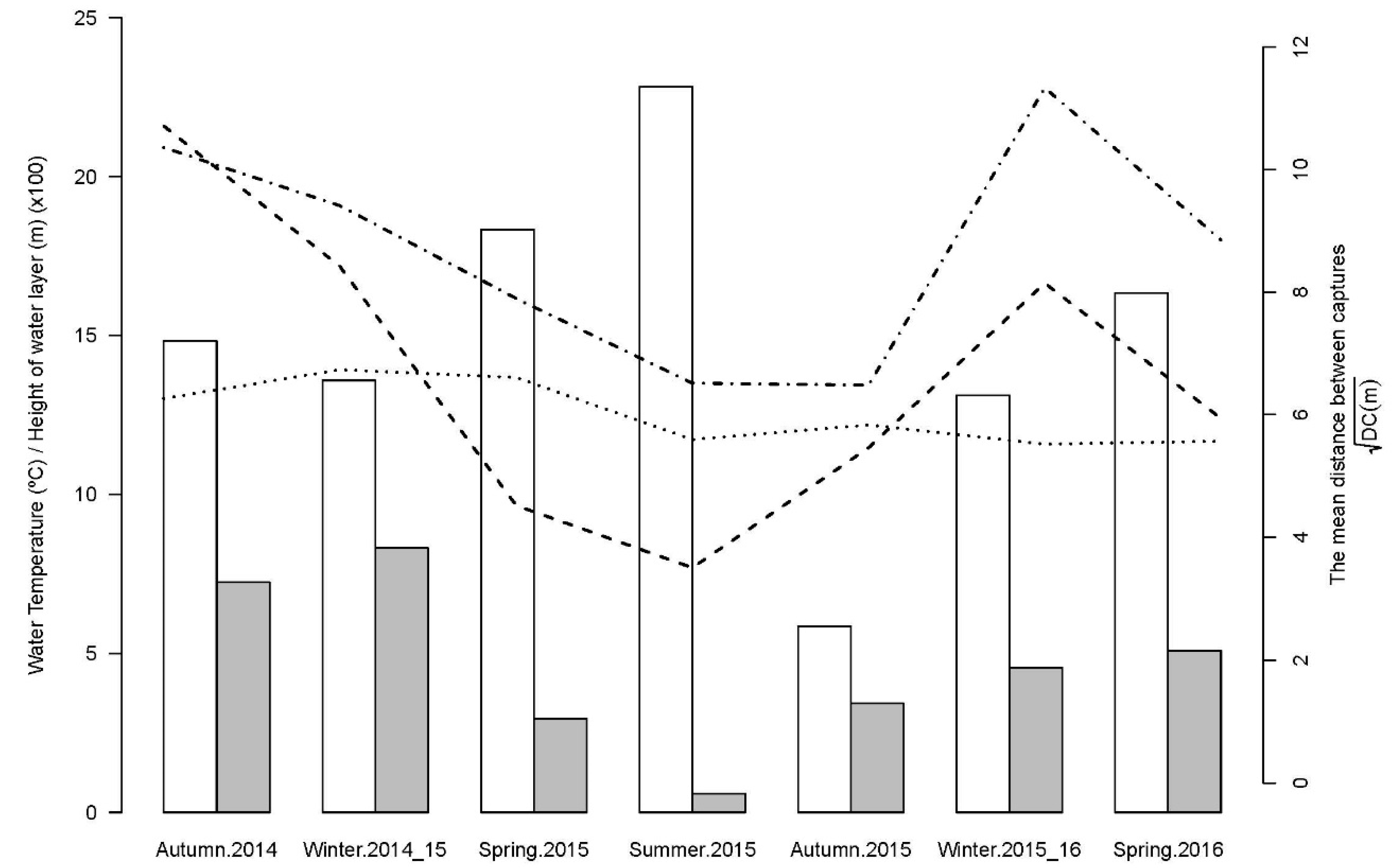
2.2.4. Factors Influencing the Extension of Eel Movements

A two-way ANOVA showed significant differences in DC (observed movements, m) between TL intervals and Season (S). The post hoc Hochberg tests detected three different groups by TL intervals, namely 25.0 to 34.9 cm, 35.0–39.9 cm, and >40.0 cm. Accordingly, TLs were grouped into these three intervals, and a subsequent two-way ANOVA was carried out, which showed significant differences between the TL intervals (F = 9.445; p = 0.000) and S (F = 3.366; p = 0.003), but not in the interactions between the TL and S variables (F = 1.264; p = 0.237). The mean DC for the eels with TL 25.0–34.9 cm was similar throughout the study period (Figure 3). Similar patterns of DC were observed for the two other TL intervals, although movements were greater in the >40.0 cm group. The distances moved were significantly larger (Hochberg test, p < 0.05) in autumn 2014 and the winters of 2014–15 and 2015–16, and significantly shorter in the spring, summer, and autumn of 2015.
The use of multinomial GLM models confirmed this pattern, indicating that the probability and size of the eel movements depended on TL, river flow (RF), and water temperature (WT) (Table 2). The best model (TL-RF) explained 31.61% (D2) of the variation of the response variable and had a relative support, as determined using Akaike weights (wi), of 60%, and the second-best model (TL-WT) explained 37% of the variation of the response variable. The remaining factors tested, as well as their interactions, had much lower support (wi), near to or below 1%. The variable with the highest relative importance (w+) was TL (Table 3), followed by RF and WT. No model obtained sufficient relative support (wi ≥ 0.9), so the inferences were made by averaging the parameters of the best models that had ΔAICc < 2 (first two models, Table 2). taking the category of movement extensions >300 m as the reference, a total of four equations were obtained with four different intersections and three slopes in common (Table 3).
The averaged model provided strong support (total wi = 0. 9739) for the odds of increasing the extension of eel movement with increasing TL and RF and decreasing it with increasing WT. Within each movement extension category, the odds of a movement (odds of occurrence, variable response) varied by a factor of eβ (slope) for each increment/decrease of one unit of each of the predictor variables. That is, the odds increased by +1.553 and +1.477 for each unit increment of TL and RF, respectively, and decreased by −0.760 for each unit increase of WT. The odds of movements in the different DCs categories (intersection; e (−αi + β1 + β2−β3)) decreased from 0.98 for movements <49.9 m to 0.07 for movements of 200.00–299.00 m relative to the reference category (>300 m), indicating a higher occurrence of movements as the extension decreased.

3. Discussion

The use of PIT tags has been recommended as one of the most suitable methods for monitoring fish populations [33,34], and has been frequently used in studies of eel behavior [9,15,35,36,37]. In our study, these tags had high survival and retention rates, and had no effect on growth or somatic condition. However, in very long-term studies (e.g., Mazel et al. [38]), a decrease in the growth of marked individuals has been observed. Additionally, we did not find any relationship between DC and Number of Days since the last capture, which suggests that eel behavior after release is not influenced by tagging and/or manipulation.
The degree of bias due to the mark–recapture methodology, and consequently also due to the distance-weighted sampling phenomenon, was low, as shown by the high average detection probability obtained for 90% of the DCs (observed movements). Additionally, the relative frequency distributions of DCs and adjusted distances after applying the Correction Factor [14] were virtually identical. Both of these are unequivocal signs of low bias in the detection of movements [7,14], and therefore also of the accurate estimation of extensions of movement range [39]. The length of the study area (1023 m) allowed large movement ranges to be observed. Nevertheless, we only detected three cases with an MDM (home range) greater than 500 m. This suggests that the true extension of the DC was smaller than what could be detected with a probability greater than 0, which explains the low deviation detected in the DC values and validates the mark–recapture methodology for the study of local eel movements. That is, a large bias in the detection of movements would be present if the specimens moved over larger distances; when the specimens mainly move over short distances, only a small number of the mark and release sites promote deviation (in our case, exclusively those sites that are closer to the borders of the sampling area), while most sites allow movement lengths to be detected with a high probability.
The frequency distribution of the DCs (observed movements) was clearly leptokurtic. In this case, with the low bias obtained, this may reflect the true size of movement, rather than being a consequence of distance-weighted sampling. This source of deviation resulting from distance-weighted sampling has been considered as the main reason for criticizing the RMP (Restricted Movement Paradigm) [27,28,29], which postulates that, despite their potential to move over long distances, most individuals in a fish population are relatively sedentary and restrict their movements to a well-defined home range. Such behavior was detected in this study and has been previously detected in other European [11,17] and American [40] eel populations, and confirms the RMP. In the absence of bias, it has been suggested that leptokurtosis may be a consequence of population heterogeneity [7,30,31], since random movements in a homogeneous population should be adjusted to a normal distribution. This heterogeneity can be caused by differences in sex, age, and social status [41,42].
In this study, the observed home range sizes (MDM) were greater than those observed in [17,21], similar to those observed in [11], or smaller than those observed in [13,16,19,43,44] in other European eel populations (Table 4). In all cases, the home range sizes observed in this study were smaller than those observed in American eel populations (Table 4), except for those observed by Ford and Mercer [40]. It has been suggested that the size of the home range of species of the genus Anguilla is related to the type of environments that they inhabit. According to Thibault et al. [20], large environments, such as estuaries and river–estuary interfaces, promote a larger movement range of A. anguilla [13,16] and A. rostrata [10,12]. In rivers, differences in home range are caused by different biotic and abiotic factors, such as habitat availability, river type, and fish population density and/or intraspecific competition [11]. In rivers with a high habitat heterogeneity, eels will not be forced to move long distances to find functional habitats [17]. Moreover, if the population density is low, the competition for space and food will also be low, and therefore the large dispersion of eels will not be promoted. In the case of the Guadiaro River, its high habitat diversity and relatively low eel population density (Fernández-Delgado et al., unpublished data) may be the reason for the observed home-range sizes.
In the studied eel population, the presence of small territories and the frequent recaptures made in the same area suggest a high degree of territoriality. This phenomenon is associated with sedentary behavior, which has been shown to promote high site fidelity in A. anguilla [11,18,19,35,48,49,50] and A. rostrata [40,45]. Eels are more efficient at exploiting environments which they already know [17] and show less ability to compete for resources outside their familiar area [51]. This territoriality is so pronounced that eels possess homing abilities and are capable of returning to their original location after they have been translocated [18,48,49,51,52].
In this study, we detected an increase in the home range (MDM) of eels with increasing body size. This phenomenon has been observed in several other eel populations (Table 4), to the degree that, in certain habitats, eel size can be considered as a good predictor of territory size [12,13]. This observation could be related to the dependence of eel feeding behavior on the eels’ body sizes; as its body length increases, an eel’s diet evolves from one based on macroinvertebrates to one based on fish [53]. This is due to a gradual increase in energy demand as the animals grow and implies the need for a bigger area to provide the necessary food resources [13].
In this study, for smaller eels (25.0 to 34.9 cm in length), a high variability and dispersion was observed in home range size (and DC values). This group showed both the largest home ranges (MDM) and a high proportion of very small territories, resulting in the lowest mean values of home range. This high variability disappeared as body size increased. This pattern could be the cause of the heterogeneity in the population and could be the reason that a leptokurtic frequency distribution was obtained for DC. Furthermore, this pattern could be related to the process of acquiring a sedentary lifestyle. This is a complex process that involves physiological and ethological changes [54]. Given the high site fidelity of the yellow eel, the process of acquiring a sedentary lifestyle involves developing a sensorial system capable of unequivocally recognizing their own territory [55]. Eel sedentarization takes place gradually and causes high variability among individuals and populations [54]. Once they have finished migratory behavior, eels become nomadic or transient [8,9], an intermediate stage in which individuals search for a territory and thus move freely and extensively through different habitats. If these nomadic/transient eels enter a mark–recapture study area, they are marked only once and never appear again [9] (Fernández-Delgado et al., unpublished data), and since their recapture rate is 0 such eels were not included in this study. However, the specimens investigated in the present study (recaptured at least once with recapture rates that allow monitoring; Fernández-Delgado et al., unpublished data) that displayed extreme values of MDM may have been in the last phase of this transient stage, in which eels begin the process of becoming sedentary. The specimens probably located an appropriate area (that was not yet their own territory) in which they moved large distances in order to search for a specific territory. Once they had found a territory, the eels investigated in this study became sedentary, and extreme movement lengths were no longer observed, being replaced by small home ranges. Since we did not mark eels with a TL < 25 cm, we could not determine the minimum length at which eels become sedentary; however, in other populations this length has been found to be 20 cm [35] or 24 cm [9]. Therefore, according to our results, we can formulate the hypothesis that, in the studied population, two distinct groups can be characterized in relation to movement patterns, home range size, and body length:
(1) Eels that are in the process of acquiring a sedentary lifestyle. At the beginning of this stage, eels make erratic movements (of up to 700 m) in the area where they will establish their territory. Once eels have established a territory, their movements become very short and do not show an environmental pattern. Individuals in this group have TLs between approximately 25 and 35 cm;
(2) Resident or sedentary eels. The eels’ movements (DCs) and home range size (MDM) increase on average as their TL increases. Their movements show an environmental pattern, they usually have TLs greater than 35 cm, and they have high site fidelity.
The concepts of territoriality and site fidelity can coexist in seasonal eel migrations [56]. In this study, migrations were not detected, although we observed a movement pattern for eels that had completed the process of acquiring sedentary behavior (TL intervals > 34.9 cm) that was linked to environmental conditions, specifically river flow and water temperature. Sedentary eels were more active with caudal increments and temperatures between 13 and 16 °C. This was observed during autumn 2014 and the winters of 2014–15 and 2015–16, when high rainfall produced large increases in river flow. In the absence of heavy rainfall, eels gradually decreased their activity (and thus their DCs). Activity reached a minimum in summer 2015, when maximum temperatures and minimum caudal flows were observed. In other populations, increases in eel activity related to river flow [57] and temperature [11,13,16,21,22,58] have been detected. At higher latitudes, eels are inactive during the cold months and increase their activity at temperatures above 16 °C [17,19]. However, at lower latitudes, such as in our study area, the temperature cycle is different. In the Guadiaro River, temperatures never dropped below 12 °C during the study period, so the eels’ inactive period was not observed. However, eel movements were lowest between July and September 2015, when the highest water temperatures were detected (20.0–24.9 °C). It has been suggested that the lower activity of eels during the summer months may be related to the higher number of light hours in these months, rather than the higher temperature, since the longer days reduce the time available for nocturnal foraging (typical of eels) and thus increase the time they remain confined to the substrate or shelters [12].
The existence of an environmental pattern in the movements of sedentary eels, as is observed in the present study, indicates that the time scale for the study of such movements is of crucial importance. Therefore, long-term studies are required to include all possible variations of home range size and movement behavior [24] as they allow a better understanding of the biology and population ecology of the European eel to be obtained, and thus facilitate more effective conservation strategies [58]. Additionally, there is a great lack of information on eel ecology in southern latitudes, despite the significant contribution of these populations to the overall stock production [59]. Thus, it is also of fundamental importance to obtain a better understanding of the variation of the key ecological processes throughout the entire distribution area of the European eel in order to improve management plans for the species.
Despite the limitations and possible bias involved in the mark–recapture methodology, we observed changes in the home range size during the yellow phase in eels and during what seems to be the process of acquiring a sedentary lifestyle. Based on the data obtained, we have formulated the hypothesis of the existence of two groups in the population (a sedentary group and another group in the process of acquiring sedentary behavior). More studies are necessary not only to confirm these results but to elucidate the sedentarization phase in depth as it is one of the least understood stages in terms of both the behavior and habitat use of eels.

4. Material and Methods
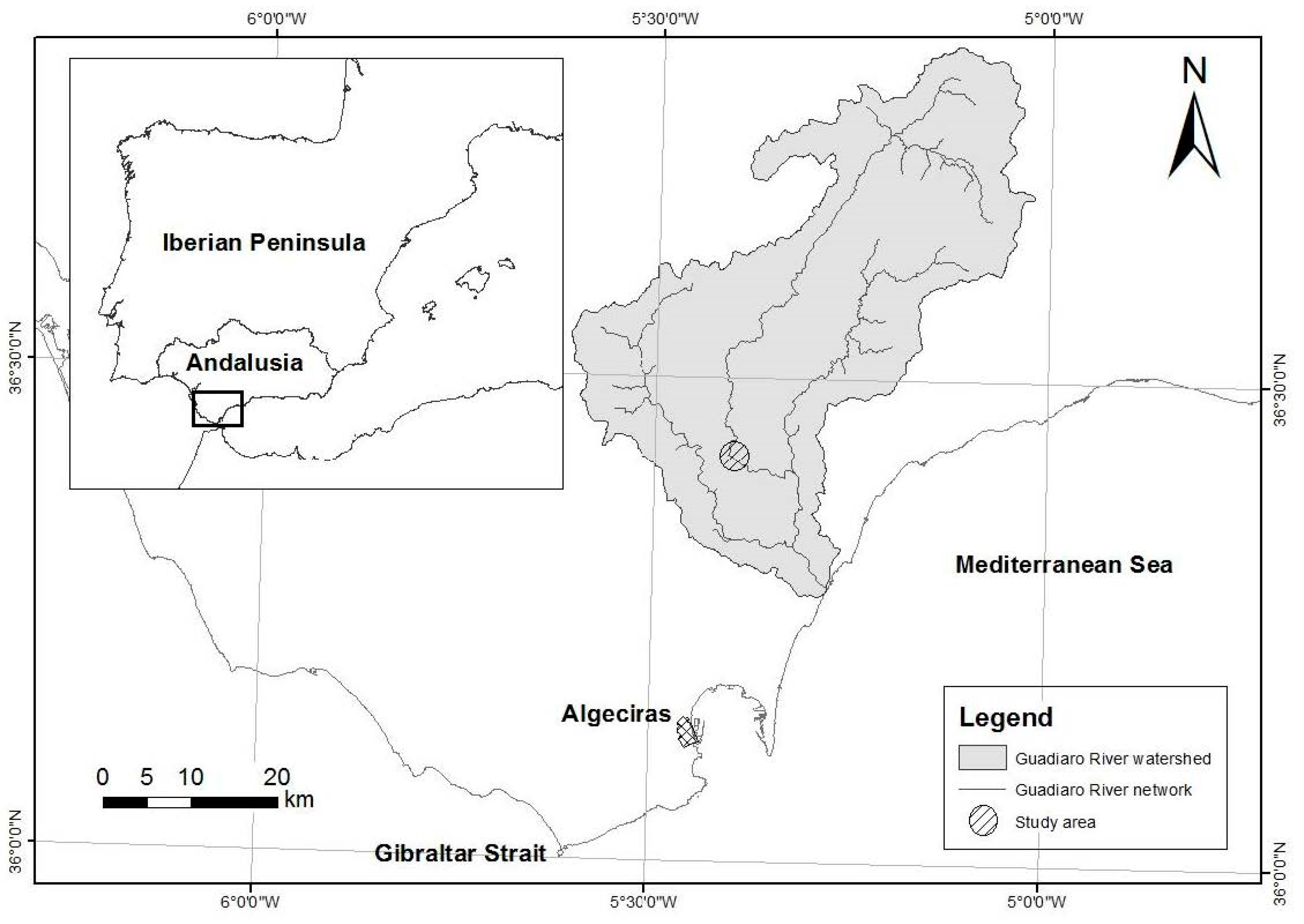
4.1. Study Area

The study was carried out in the Guadiaro River, Southern Spain (UTM 30S 284525; 4033181 -SRC: ETRS89, EPSG 25830-). The river’s hydrographic basin is 82 km in length, covers an area of 1505 km2, and discharges into the Mediterranean Sea (Figure 4).
The Guadiaro River has a sub-humid thermo-Mediterranean climate with an average temperature of 17 °C and an average annual precipitation of 725 mm, with episodes of heavy rain. The river’s water flow is permanent throughout the year due to the regulatory function of karst upwellings in the upper section of the hydrographic basin, although it varies due to large floods in winter, with minimum values being observed at the end of summer [60]. In the Guadiaro River, the European eel coexists with the sand smelt (Atherina boyeri, Risso, 1810), the Southern Iberian barbel (Luciobarbus sclateri, Günther, 1868), the southern straight-mouth nose (Pseudochondrostoma willkommi, Steindachner, 1866), an endangered species of chub endemic to Southern Spain (Squalius malacitanus, Doadrio and Carmona, 2006), the sea lamprey (Petromyzon marinus, Linnaeus, 1758), and the grey mullet (Liza ramada, Risso, 1827). There are also several introduced species of fish, although at low population densities: the topmouth gudgeon (Pseudorasbora parva, Temminck and Schlegel, 1846), the carp (Cyprinus carpio, Linnaeus, 1758), and the mosquitofish (Gambusia holbrooki, Girard, 1859).
The water quality of the Guadiaro River is high, mainly due to the fact that a large part of the river basin is located inside the boundaries of a large natural forested area, the Alcornocales Natural Park. Additional factors which contribute to the river’s high water quality are the absence of large dams and the fact that the region’s riparian vegetation has been well conserved. Most of the river basin (56%) belongs to the European Commission’s Natura 2000 Network.
In this study, a segment of the middle reaches of the Guadiaro River (located approximately 28 km from the Guadiaro River estuary) with a length of 1023 m and a mean width of 10 m (corresponding to an area of ≅1.6 ha) was sampled monthly between October 2014 and June 2016. The segment was chosen as it has a high aquatic habitat heterogeneity, with pools, runs, and riffles of different sizes and abundant shelter for fish. The substrate is mostly mud or sand, however there are also some areas with pebbles of different sizes, especially in riffles and runs. The water depth ranged between 20 cm (runs) and 185 cm (pools). The minimum water temperature was measured in December 2015 (12.0 °C) and the maximum water temperature in July 2015 (24.9 °C). Levels of dissolved oxygen varied from 5.69 mg L−1 (August 2015) to 11.9 mg L−1 (December 2015) and water conductivity varied from 307 μS cm−1 (April 2016) to 606 μS cm−1 (September 2015). The weather conditions varied greatly between seasons throughout the study period. During autumn and winter of 2014–2015, rainfall was unusually heavy (monthly mean of 118.5 mm), leading to substantial increases in the river flow. The rest of the sampling period was mostly dry with brief episodes of heavy rain.

4.2. Mark–Recapture Study

4.2.1. Tag Retention

A study of eel movements was carried out using PIT tags whose effects on eel survival and fitness and retention rates in eels had previously been tested in the laboratory. A total of 182 European eels collected from the marshlands of the Guadalquivir River, southwestern Iberian Peninsula (UTM 30S 213060; 4096063 -SRC: ETRS89, EPSG 25830-), were reared in a 4000 L tank of salt water (30 g/L ClNa; 20 °C; 6 mg/L O2; pH = 7) for nine months. The water was renewed every 5 h and treated using biological filters and ultraviolet light sterilization. All experimental procedures were conducted in compliance with the European legislation for the protection of animals used for scientific purposes (Directive 2010/63/EU). After a one-month acclimatization period, the eels were anaesthetized in a 1:1000 solution of clove oil dissolved (1:10) in ethanol (70%) [61]. The TL (cm) and body mass (M, g) were recorded for each specimen. A random sample of 100 individuals were tagged with PIT tags (M.U.S.I.C.C.®, Avid Identification System Inc., Norco, CA, USA) with dimensions of 8 × 2.1 mm (n = 49; X ¯ T L = 30.0 ± 1.0 cm at the 95% C.I.; range = 23.4–44.6 cm) or 12.0 × 2.1 mm (n = 51; X ¯ T L = 29.7 ± 0.8 cm at the 95% C.I.; range = 23.6–38.0 cm), leaving 82 eels untagged ( X ¯ T L = 30.3 ± 0.8 cm at the 95% C.I.; range = 22.5–41.8 cm). PIT tags were injected into the dorsal musculature 1–2 cm behind the beginning of the dorsal fin and parallel to the axis of the vertebral column. Care was taken to avoid the vertebral column and the lateral line. The insertion site was disinfected with Betadine® gel (MEDA Manufacturing, Bordeaux, France). Eels were anaesthetized every 30 days (see above), after which TL and M were recorded and the animals were examined for tag retention using a PIT tag reader (PowerTracker V®, Avid Identification System Inc.). The Residual Condition Index (Kr) was calculated using standardized residuals obtained from Log (TL)–Log (M) regression [62].
A covariance analysis was carried out using M as the response variable, and T, TL, the presence or absence of a PIT, and PIT size (P) as predictor variables.

4.2.2. Sampling Protocol

The sampling framework of the Robust Design [63,64] was chosen for the mark–recapture study. The stretch of river that comprised the study area was divided into two sections—A and B. The sampling period was six days. On the first day, a total of 50 numbered fyke nets were set in section A for 24 h, distributed on both river banks and separated from each other by approximately 20 m; each net was 2.5 m in length, and 25 of the nets had a 10 mm mesh size while the other 25 had a 7 mm mesh size. Subsequently, the nets were removed and installed in section B for another 24-h period. This process was repeated until three 24-h cycles had been completed in each section. We assumed that the absence of fishing for one day facilitated a homogeneous mixture of marked and unmarked individual eels. The same methodology was carried out every month from October 2014 to June 2016, thus obtaining data of eel movements at different time scales (daily, monthly, and seasonal). The eels caught in each fyke net were transferred to a labeled net bag and their coordinates (UTM) were recorded. This made it possible to relate each individual to the exact position where it was caught. The eels were anesthetized and their TL (cm), M (g), and external measurements proposed by Durif et al. [32] for determining the maturation stage (mm) were recorded, both for the first capture and for the recaptures. Eels with a TL larger than 25 cm were marked using PIT tags or examined for the presence of tags, following the protocol described above. Once eels had been processed, they were released in exactly the same place where they were captured.

4.2.3. Data Analysis

A total of 722 eels were tagged throughout the study period. Of these, 389 were recaptured. For the study of movements and home ranges, data were collected from 296 individuals selected according to the following criteria: First, eels which were recaptured one or more times at least one month after their first capture. In this way, the influence of transient individuals (nomadic individuals who had not yet begun the process of acquiring sedentary behavior [8,9] or migrating silver eels) was avoided; and second, eels in silvering stages were excluded. All data were obtained from yellow eels in the FI to FIII maturation stages [32]. Not all of the 296 eels were monitored during the entire study period. In the 23 months of the study period, new sedentary eels settled in the study area, and their data were incorporated; additionally, other eels started the silvering process, and their data were excluded as indicated above.
Statistical analysis was performed with SPSS v. 23 (IBM® SPSS® Statistics, 2015; International Business Machines Corporation, New York, USA) and the R software 3.3.2 (R Development Core Team, 2016). In general, statistical significance was assessed at p < 0.05; other significance levels are indicated when appropriate.
In order to estimate the degree of bias due to the mark–recapture methodology, and consequently the degree of bias due to the distance-weighted sampling phenomenon, Albanese’s procedure was used [23]. This involves constructing a theoretical distribution of the probabilities of detecting movements based on their length (in this case, every 50 m moved) and later comparing this with the observed distribution of movements. Additionally, a Correction Factor [14] was applied to account for variations in the sampling intensity with distance.
The following two variables were obtained to characterize the movement patterns:
(1)
DC (m; Distance between Captures or observed movements): distance moved in meters between two consecutive captures. It can be negative (downstream) or positive (upstream). DC was tested against the value of D between two consecutive captures;
(2)
MDM (m; Maximum Distance Moved or home range): difference between the extreme positions occupied by an individual during the study. Only the longitudinal component was considered [4,11].
The two previous variables were related to the TL at the time when the movement was detected (for DC) and the mean TL of the total number of recaptures (for MDM). Body lengths were divided into the following intervals: 25–29.9 cm, 30.0–34.9 cm, 35.0–39.9 cm, 40.0–49.9 cm, and >50 cm. MDM was studied using the following descriptive statistical methods: the usual central tendency; dispersion measures; 5% trimmed mean (in which 5% of the extreme values are discarded); M-estimators—robust alternatives to the weighted mean (Huber’s M-estimator, Andrews’ wave estimator, Hampel’s re-descending M-estimator, and Tukey’s bi-weight estimator); the interquartile range (IQR, middle 50% of values) in a Tukey boxplot; and cases outside the 1.5 IQR (outliers) and 3 IQR or more of the bottom or top quartiles (extreme values).
We calculated the MR (Movement Rate) of the eels to study the variation in the Distance between Captures (observed movements) in relation to body size. Based on the width of the intervals used in the study of the theoretical and DC distributions of movements (see above), at each recapture, the distance in meters to the position of the previous catch was used to classify the individual as either static (<50 m, first interval) or mobile (>50 m, the rest of the intervals). MR was calculated as the proportion of movements >50 m to the total number of movements detected in the population.
To explore factors influencing the DC (m, observed movements), as a first step, a two-way ANOVA was used for individuals with two or more recaptures. To homogenize the variances, the response variable used was the square root of DC (absolute value). The following classification variables were used: TL interval (cm) and S, a dummy variable with the function of summarizing environmental variables involved in the possible variation of the movements in an annual cycle. For S, values of 1 to 7 were given to represent the seven seasons covered by the study period. The post hoc Hochberg test for unequal samples was used.
Using the information obtained in the previous step, further analysis was performed using Multinomial Generalized Linear Models (GLM) with an accumulated logit link function [65,66]. The response variable (DC, m) was divided into five categories: <49.9 m; 50–99.9 m; 100–199.9 m; 200–299.9 m; and >300 m. The following predictor variables were tested:
(1)
The TL (cm) of the individual when movement was detected;
(2)
CPUE (Catch per unit effort): the average number of specimens captured in a 24-h cycle, interpreted as an indicator of the degree of activity in eels.
Several environmental variables were considered which a priori could be representative of the length of the DC:
(1)
River Flow (RF, m): mean river level (height of the water layer in meters) from four days before the beginning of sampling until its completion;
(2)
Increase in RF (ΔRF, m): the difference between the maximum and minimum water levels in the four days prior to the beginning of sampling;
(3)
Water Temperature (WT, °C): measured early in the morning (at around 09:00) on each day of sampling.
For RF and ΔRF, flow data were obtained from the Automatic Hydrological Data Collection System SAIH Hidrosur (http://www.redhidrosurmedioambiente.es).
The collinearity between the predictor variables was previously verified using the following collinearity diagnostics: variance inflation factor (VIF), tolerance statistics (1/VIF), and the correlation matrix of all predictor variables. The results indicate that, except for TL, all the independent variables were collinear with each other at p < 0.01. Therefore, the models were constructed separately for TL and each of the environmental variables.
The overall significance of the models was tested with an Omnibus test based on the chi-squared likelihood ratio of a particular model. This test compares the fitted model against the intercept-only model. The amount of variation in the response variable that is explained by a model (D2) was calculated using the deviance as D2 = (deviance of intercept-only model—deviance model)/deviance of intercept-only model).
The AIC corrected for small samples (AICc), which provides an estimate of the quality of a particular model relative to each of the other candidate models [67], was used for model selection. The relative strength of the evidential support provided by each model was evaluated using Akaike weights [67]. In the case that a model providing strong support (wi > 0.9) could not be found among the tested models, multi-model inference (MMI) was used, which was carried out using the models with a difference in AICc (ΔAICc) smaller than 2 [67,68]. Finally, the relative importance of each variable (w+) was calculated [67] using the support value of each model (wi).

Author Contributions

C.F.-D. supervised the study. M.H. analyzed the data. M.H. and C.F.-D. wrote the manuscript. M.H., R.M.-V., R.D.M.R. and C.F.-D contributed to the interpretation of results and revised the final version of the manuscript.

Funding

This study was funded through a collaborative agreement between the University of Córdoba and the Andalusian Environmental Regional Agency in the framework of the Regional Eel Management Program.

Acknowledgments

We are grateful for the invaluable help of Manuel Ruíz Sánchez with the field sampling and of Juan Antonio Calderón and the Integrated Center for Professional Training (CIFP) Zaporito with the laboratory experiments.

Conflicts of Interest

The author declares no conflict of interest.

References

  1. ICES. Report of the Joint EIFAAC/ICES/GFCM Working Group on Eel, 3–7 November 2014, Rome, Italy; ICES CM 2014/ACOM:18; ICES: Copenhagen, Denmark, 2014; p. 203. [Google Scholar]
  2. ICES. Report of the Joint EIFAAC/ICES/GFCM Working Group on Eel (WGEEL), 24 November–2 December 2015, Antalya, Turkey; ICES CM 2015/ACOM:18; ICES: Copenhagen, Denmark, 2015; p. 130. [Google Scholar]
  3. ICES. Report of the Working Group on Eels (WGEEL), 15–22 September 2016, Cordoba, Spain; ICES CM 2016/ACOM:19; ICES: Copenhagen, Denmark, 2016; p. 107. [Google Scholar]
  4. Hill, J.; Grossman, G.D. Home Range Estimates for Three North American Stream Fishes. Copeia 1987, 1987, 376–380. [Google Scholar] [CrossRef]
  5. Belica, L.A.T.; Rahel, F.J. Movements of creek chubs, Semotilus atromaculatus, among habitat patches in a plains stream. Ecol. Freshw. Fish 2008, 17, 258–272. [Google Scholar] [CrossRef]
  6. Smithson, E.B.; Johnston, C.E. Movement patterns of stream fishes in an Ouachita highlands stream: An examination of the restricted movement paradigm. Trans. Am. Fish. Soc. 1999, 128, 847–853. [Google Scholar] [CrossRef]
  7. Skalski, G.T.; Gilliam, J.F. Modeling Diffusive Spread in a Heterogeneous Population: A Movement Study with Stream Fish. Ecology 2000, 81, 1685–1700. [Google Scholar] [CrossRef]
  8. Feunteun, E.; Laffaille, P.; Robinet, T.; Briand, C.; Baisez, A.; Olivier, J.-M.; Acou, A. A Review of Upstream Migration and Movements in Inland Waters by Anguillid Eels: Toward a General Theory. In Eel Biology; Aida, K., Tsukamoto, K., Yamauchi, K., Eds.; Springer: Tokyo, Japan, 2003; pp. 191–213. [Google Scholar]
  9. Imbert, H.; LaBonne, J.; Rigaud, C.; Lambert, P. Resident and migratory tactics in freshwater European eels are size-dependent. Freshw. Biol. 2010, 55, 1483–1493. [Google Scholar] [CrossRef]
  10. Hedger, R.D.; Dodson, J.J.; Hatin, D.; Caron, F.; Fournier, D.; Hedger, R. River and estuary movements of yellow-stage American eels Anguilla rostrata, using a hydrophone array. J. Fish Biol. 2010, 76, 1294–1311. [Google Scholar] [CrossRef] [PubMed]
  11. Ovidio, M.; Seredynski, A.L.; Philippart, J.-C.; Matondo, B.N. A bit of quiet between the migrations: The resting life of the European eel during their freshwater growth phase in a small stream. Aquat. Ecol. 2013, 47, 291–301. [Google Scholar] [CrossRef]
  12. Béguer-Pon, M.; Castonguay, M.; Benchetrit, J.; Hatin, D.; Legault, M.; Verreault, G.; Dodson, J.J. Large-scale, seasonal habitat use and movements of yellow American eels in the St. Lawrence River revealed by acoustic telemetry. Ecol. Freshw. Fish 2015, 24, 99–111. [Google Scholar] [CrossRef]
  13. Barry, J.; Newton, M.; Dodd, J.A.; Hooker, O.E.; Boylan, P.; Lucas, M.C.; Adams, C.E. Foraging specialisms influence space use and movement patterns of the European eel Anguilla anguilla. Hydrobiologia 2016, 766, 333–348. [Google Scholar] [CrossRef]
  14. Porter, J.H.; Dooley, J.L. Animal Dispersal Patterns: A Reassessment of Simple Mathematical Models. Ecology 1993, 74, 2436–2443. [Google Scholar] [CrossRef]
  15. Riley, W.D.; Walker, A.M.; Bendall, B.; Ives, M.J. Movements of the European eel (Anguilla anguilla) in a chalk stream. Ecol. Freshw. Fish 2011, 20, 628–635. [Google Scholar] [CrossRef]
  16. Walker, A.M.; Godard, M.J.; Davison, P. The home range and behaviour of yellow-stage European eel Anguilla anguilla in an estuarine environment. Aquat. Conserv. 2014, 24, 155–165. [Google Scholar] [CrossRef]
  17. Baras, E.; Jeandrain, D.; Serouge, B.; Philippart, J.C. Seasonal variations of time and space utilisation by radiotagged yellow eels Anguilla anguilla (L.) in a small stream. Hydrobiologia 1998, 371, 187–198. [Google Scholar] [CrossRef]
  18. Le Pichon, C.; Coustillas, J.; Zahm, A.; Bunel, M.; Gazeau-Nadin, C.; Rochard, E. Summer use of the tidal freshwaters of the River Seine by three estuarine fish: Coupling telemetry and GIS spatial analysis. Estuar. Coast. Shelf Sci. 2017, 196, 83–96. [Google Scholar] [CrossRef]
  19. Verhelst, P.; Reubens, J.; Pauwels, I.; Buysse, D.; Aelterman, B.; Van Hoey, S.; Goethals, P.; Moens, T.; Coeck, J.; Mouton, A. Movement behaviour of large female yellow European eel (Anguilla anguilla L.) in a freshwater polder area. Ecol. Freshw. Fish 2018, 27, 471–480. [Google Scholar] [CrossRef]
  20. Thibault, I.; Dodson, J.J.; Caron, F. Yellow-stage American eel movements determined by microtagging and acoustic telemetry in the St Jean River watershed, Gaspé, Quebec, Canada. J. Fish Biol. 2007, 71, 1095–1111. [Google Scholar] [CrossRef]
  21. LaBar, G.W.; Hernando Casal, J.A.; Fernández Delgado, C. Local movements and population size of European eels, Anguilla anguilla, in a small lake in south-western Spain. Environ. Biol. Fishes 1987, 19, 111–117. [Google Scholar] [CrossRef]
  22. Sinha, V.R.P.; Jones, J.W. The European Freshwater Eel; Liverpool University: Liverpool, UK, 1975. [Google Scholar]
  23. Albanese, B.; Angermeier, P.L.; Gowan, C. Designing Mark–Recapture Studies to Reduce Effects of Distance Weighting on Movement Distance Distributions of Stream Fishes. Trans. Am. Fish. Soc. 2003, 132, 925–939. [Google Scholar] [CrossRef]
  24. Crook, D.A. Is the home range concept compatible with the movements of two species of lowland river fish? J. Anim. Ecol. 2004, 73, 353–366. [Google Scholar] [CrossRef]
  25. Baker, M.; Nur, N.; Geupel, G.R. Correcting biased estimates of dispersal and survival due to limited study area: Theory and application using wren tits. Condor 1995, 7, 663–674. [Google Scholar] [CrossRef]
  26. Koenig, W.D.; Van Vuren, D.; Hooge, P.N. Detectability, philopatry, and the distribution of dispersal distances in vertebrates. Trends Ecol. Evol. 1996, 11, 514–517. [Google Scholar] [CrossRef]
  27. Gerking, S.D. The Restricted Movement of Fish Populations. Biol. Rev. 1959, 34, 221–242. [Google Scholar] [CrossRef]
  28. Gowan, C.; Young, M.K.; Fausch, K.D.; Riley, S.C. Restricted movement in resident stream salmonids: A paradigm lost? Can. J. Fish. Aquat. Sci. 1994, 51, 2626–2637. [Google Scholar] [CrossRef]
  29. Gowan, C.; Fausch, K.D. Mobile brook trout in two high-elevation Colorado streams: Re-evaluating the concept of restricted movement. Can. J. Fish. Aquat. Sci. 1996, 53, 1370–1381. [Google Scholar] [CrossRef]
  30. Fraser, D.F.; Gilliam, J.F.; Daley, M.J.; Le, A.N.; Skalski, G.T. Explaining Leptokurtic Movement Distributions: Intra population Variation in Boldness and Exploration. Am. Nat. 2001, 158, 124–134. [Google Scholar] [CrossRef] [PubMed]
  31. Rodríguez, M.A. Restricted Movement in Stream Fish: The Paradigm Is Incomplete, Not Lost. Ecology 2002, 83, 1–13. [Google Scholar] [CrossRef]
  32. Durif, C.; Guibert, A.; Elie, P. Morphological discrimination of the silvering stages of the European eel. Am. Fish. Soc. 2009, 58, 103–111. [Google Scholar]
  33. Bolland, J.D.; Cowx, I.G.; Lucas, M.C. Evaluation of VIE and PIT tagging methods for juvenile cyprinid fishes. J. Appl. Ichthyol. 2009, 25, 381–386. [Google Scholar] [CrossRef]
  34. Hirt-Chabbert, J.A.; Young, O.A. Effects of surgically implanted PIT tags on growth, survival and tag retention of yellow shortfin eels Anguilla australis under laboratory conditions. J. Fish Biol. 2012, 81, 314–319. [Google Scholar] [CrossRef]
  35. Laffaille, P.; Acou, A.; Guillouët, J. The yellow European eel (Anguilla anguilla L.) may adopt a sedentary lifestyle in inland freshwaters. Ecol. Freshw. Fish 2005, 14, 191–196. [Google Scholar] [CrossRef]
  36. Chadwick, S.; Knights, B.; Thorley, J.L.; Bark, A. A long-term study of population characteristics and downstream migrations of the European eel Anguilla anguilla (L.) and the effects of a migration barrier in the Girnock Burn, north-east Scotland. J. Fish Biol. 2007, 70, 1535–1553. [Google Scholar] [CrossRef]
  37. Charrier, F.; Mazel, V.; Caraguel, J.M.; Abdallah, Y.; Le Gurun, J.; Legault, A.; Laffaille, P. Escapement of a silver-phase eel population, Anguilla anguilla, determined from fishery in a Mediterranean lagoon (Or, France). ICES J. Mar. Sci. 2012, 69, 30–33. [Google Scholar] [CrossRef]
  38. Mazel, V.; Charrier, F.; Legault, A.; Laffaille, P. Long-term effects of passive integrated transponder tagging (PIT tags) on the growth of the yellow European eel (Anguilla anguilla (Linnaeus, 1758)). J. Appl. Ichthyol. 2013, 29, 906–908. [Google Scholar] [CrossRef]
  39. Alldredge, P.; Gutierrez, M.; Duvernell, D.; Schaefer, J.; Brunkow, P.; Matamoros, W. Variability in movement dynamics of topminnow (Fundulus notatus and F. olivaceus) populations. Ecol. Freshw. Fish 2011, 20, 513–521. [Google Scholar] [CrossRef]
  40. Ford, T.E.; Mercer, E. Density, size distribution and home range of American eels, Anguilla rostrata, in a Massachusetts salt marsh. Environ. Biol. Fishes 1986, 17, 309–314. [Google Scholar] [CrossRef]
  41. Armstrong, J.D.; Braithwaite, V.A.; Huntingford, F.A. Spatial Strategies of Wild Atlantic Salmon Parr: Exploration and Settlement in Unfamiliar Areas. J. Anim. Ecol. 1997, 66, 203–211. [Google Scholar] [CrossRef]
  42. Gilliam, J.F.; Fraser, D.F. Corridor movement: Enhancement by predation threat, habitat structure and disturbance. Ecology 2001, 82, 258–273. [Google Scholar] [CrossRef]
  43. Mann, H. Über das rückkehrvermogen verpflantzer fluss-aal. Arch. Fischereiwiss. 1965, 15, 177–185. [Google Scholar]
  44. McGovern, P.; McCarthy, T.K. Local movements of freshwater eels (Anguilla anguilla L.) in western Ireland. In Wildlife Telemetry: Remote Sensing and Monitoring of Animals; Priede, I.G., Swift, S.M., Eds.; Ellis Horwood: Chichester, UK, 1992; pp. 319–327. [Google Scholar]
  45. LaBar, G.W.; Facey, D.E. Local Movements and Inshore Population Sizes of American Eels in Lake Champlain, Vermont. Trans. Am. Fish. Soc. 1983, 112, 111–116. [Google Scholar] [CrossRef]
  46. Bozeman, E.L.; Helfman, G.S.; Richardson, T. Population Size and Home Range of American Eels in a Georgia Tidal Creek. Trans. Am. Fish. Soc. 1985, 114, 821–825. [Google Scholar] [CrossRef]
  47. Dutil, J.-D.; Giroux, A.; Kemp, A.; Lavoie, G.; Dallaire, J.-P. Tidal Influence on Movements and on Daily Cycle of Activity of American Eels. Trans. Am. Fish. Soc. 1988, 117, 488–494. [Google Scholar] [CrossRef]
  48. Parker, S. Homing Ability and Home Range of Yellow-Phase American Eels in a Tidally Dominated Estuary. J. Mar. Biol. Assoc. UK 1995, 75, 127–140. [Google Scholar] [CrossRef]
  49. Rossi, R.; Bianchini, M.; Carrieri, A.; Franzoi, P. Observations on movements of yellow eels, Anguilla anguilla L., after displacement from coastal waters to sea. J. Fish Biol. 1987, 31, 155–164. [Google Scholar] [CrossRef]
  50. Baisez, A. Optimisation des suivis des indices d’abondances et des structures de taille de l’anguille europeénne (Anguilla anguilla, L.) dans un marais endigué de la côte atlantique: Relations espèce–habitat. Ph.D. Thesis, University of Toulouse, Toulouse, France, 2001. [Google Scholar]
  51. Lamothe, P.J.; Gallagher, M.; Chivers, D.P.; Moring, J.R. Homing and Movement of Yellow-phase American Eels in Freshwater Ponds. Env. Biol. Fishes 2000, 58, 393–399. [Google Scholar] [CrossRef]
  52. Tesch, F.-W. Homing of eels (Anguilla anguilla) in the southern North Sea. Mar. Biol. 1967, 1, 2–9. [Google Scholar] [CrossRef]
  53. Laffaille, P.; Feunteun, E.; Baisez, A.; Robinet, T.; Acou, A.; Legault, A.; Lek, S. Spatial organisation of European eel (Anguilla anguilla L.) in a small catchment. Ecol. Freshw. Fish 2003, 12, 254–264. [Google Scholar] [CrossRef]
  54. Edeline, E.; Dufour, S.; Elie, P. Proximate and Ultimate Control of Eel Continental Dispersal. In Spawning Migration of the European Eel; Van den Thillart, G., Dufour, S., Rankin, J.C., Eds.; Springer: Berlin/Heidelberg, Germany, 2009; pp. 433–461. [Google Scholar]
  55. Braithwhaite, V.A.; De Perera, B. Short-range orientation in fish: How fish map space. Mar. Fresh. Behav. Physiol. 2006, 39, 37–47. [Google Scholar] [CrossRef]
  56. Knights, B. Eel biology and the status of recruitment and stocks. In Proceedings of the 2009 Eel Conference; Eel Management: The State of the Art; Bunt, D.A., Don, A.M., Eds.; Institute of Fisheries Management: Kingston upon Hull, UK, 2011; pp. 22–40. [Google Scholar]
  57. Hammond, S.D.; Welsh, S.A. Seasonal Movements of Large Yellow American Eels Downstream of a Hydroelectric Dam, Shenandoah River, West Virgina. In Eels at the Edge: Science, Status, and Conservation Concerns; Casselman, J.M., Cairns, D.K., Eds.; American Fisheries Society: Bethesda, MD, USA, 2009; Volume 58, pp. 309–323. [Google Scholar]
  58. Cullen, P.; McCarthy, T.K. Eels (Anguilla anguilla (L.)) of the lower River Shannon, with particular reference to seasonality in their activity and feeding ecology biology and environment. Proc. R. Ir. Acad. 2007, 107, 87–94. [Google Scholar] [CrossRef]
  59. Dekker, W. Did lack of spawners cause the collapse of the European eel, Anguilla anguilla? Fish. Manag. Ecol. 2003, 10, 365–376. [Google Scholar] [CrossRef]
  60. Grupo de Investigación Integrada en Áreas Litorales. Gestión Integrada de Zonas Costeras y Cuencas Hidrográficas: Introducción a un Caso de Estudio; Universidad de Cádiz: Cádiz, Spain, 2009. [Google Scholar]
  61. Durif, C.; Dufour, S.; Elie, P. The silvering process of Anguilla anguilla: A new classification from the yellow resident to the silver migrating stage. J. Fish Biol. 2005, 66, 1025–1043. [Google Scholar] [CrossRef]
  62. Sutton, S.G.; Bult, T.P.; Haedrich, R.L. Relationships among Fat Weight, Body Weight, Water Weight, and Condition Factors in Wild Atlantic Salmon Parr. Trans. Am. Fish. Soc. 2000, 129, 527–538. [Google Scholar] [CrossRef]
  63. Pollock, K.H. A Capture-Recapture Design Robust to Unequal Probability of Capture. J. Wildl. Manag. 1982, 46, 752–757. [Google Scholar] [CrossRef]
  64. Kendall, W.L.; Nichols, J.D.; Hines, J.E. Estimating Temporary Emigration Using Capture–Recapture Data with Pollock’s Robust Design. Ecology 1997, 78, 563–578. [Google Scholar]
  65. McCullagh, P.; Nelder, J.A. Generalized Linear Models. Monographs on Statistics and Applied Probability 37; Chapman & Hall: London, UK, 1989. [Google Scholar]
  66. Lawal, H.B. Categorical Data Analysis with SAS and SPSS Applications; Erlbaum Associates Publishers: Mahwah, NJ, USA, 2003. [Google Scholar]
  67. Burnham, K.P.; Anderson, D.R. Model Selection and Multi-Model Inference: A Practical Information-Theoretic Approach; Springer: New York, NY, USA, 2002. [Google Scholar]
  68. Buckland, S.T.; Burnham, K.P.; Augustin, N. Model Selection: An Integral Part of Inference. Biometrics 1997, 53, 603–618. [Google Scholar] [CrossRef]
Figure 1. Frequency distributions: Theoretical probabilities of detection of movements given the movement extension. Possible movements sampled shown by white bars; Distance between Captures (DC, observed movements, black bars); Adjusted frequency of movements at each distance obtained after applying the Correction Factor (grey bars). Point 0 represents the absence of movement or movements smaller than 50 m.
Fishes 04 00043 g001
Figure 2. Absolute values (in m) for specimens recaptured once or more during the study period: (a) Distance between Captures (DC, observed movements), outliers between 158.70 and 246.91 m (dotted line) and extreme values from this last distance; (b) Maximum Distance Moved (MDM), outliers between 204.63 m and 318.3 m (dotted line) and extreme values from this distance onwards.
Fishes 04 00043 g002
Figure 3. Mean distances moved (square root of DC, observed movements, m) during the study period by length interval in specimens recaptured more than once. Dotted line: eels with TL < 34.9 cm; dashed line: eels with TL between 35–39.9 cm; dot-dash line: eels with TL > 40 cm. Also shown seasonal averages of water temperature (°C, white bars) and height of water layer (×100 m, grey bars).
Fishes 04 00043 g003
Figure 4. Maps showing the geographical location of the study area and the Guadiaro River watershed.
Fishes 04 00043 g004
Table 1. Maximum Distance Moved (MDM, home range) descriptive statistics by length intervals (mean body length (total length, TL) of the total number of recaptures) in the studied eel population of the Guadiaro River. Data are from individuals with one or more recaptures. CV = Coefficient of variation.
Total Length
(cm)
NMean ± 95% C.I.
(m)
5% Trimmed
Mean (m)
M–Estimators
(m)
Median
(m)
Range
(m)
CVOutliers
(m)
Extreme Values
(m)
Mean Area ± 95% C.I.
(m2)
25.0–29.913765.47 ± 17.9847.5524.38–32.0226.49707.041.63165.08–268.11319.51–707.041023.97 ± 281.21
30.0–34.912278.67 ± 19.6562.436.96–44.5039.79622.091.39197.21–271.42300.05–622.551230.42 ± 307.33
35.0–39.91899.79 ± 51.9293.1340.06–58.9348.72316.731.05NoNo1560.74 ± 812.04
40.0–49.913158.61 ± 79.56151.1475.94–99.2784.13363.810.83NoNo2480.70 ± 1244.34
>50.No06258.76 ± 99.07257.44249.30–252.58242.21264.440.37NoNo4047.08 ± 1549.48
Table 2. Multinomial GLM models with Akaike weights (wi) > 0 ordered by increasing Akaike’s Information Criterion adjusted for small sample size (AICc), for the odds and extent of movements detected in the Guadiaro River eel population between October 2014 and June 2016. ΔAICc: Difference in ΔAICc compared to the best model; wi: Akaike weights.TL = total length (cm), RF= river flow (level in meters), ΔRF = increase in river flow (m) and WT = water temperature (°C).
ModelOmnibus TestDevianceAICcΔAICcwi
y = intercept-TL-RF<0.05436.907768.5760.0000.6053
y = intercept-TL-WT<0.05489.689769.5680.9920.3686
y = intercept-TL-ΔRF<0.05599.930776.5676.9990.0111
y = intercept-TL<0.05578.992777.5779.0010.0067
y = intercept-TL-ΔRF-interaction<0.05612.624778.3789.8020.0045
y = intercept-TL-RF-interaction<0.05607.686779.68411.1080.0023
y = intercept-TL-WT-interaction<0.05605.243781.412.8240.0010
y = intercept-RF<0.05625.660784.82816.2520.0002
y = intercept-WT<0.05629.322784.90716.3310.0002
y = intercept 638.827791.32822.7520.0000
Table 3. Results of Multi-model inference from the models TL-RF and TL-WT (ΔAICc < 2). Parameter estimates, 95% C.I. and the relative importance of each variable (w+) (Total Length, River Flow and Water Temperature) for the odds and extent of eel movements (m) in the Guadiaro River population between October 2014 and June 2016.
Parameter Estimate95% CIw+
α Intercepts (Movements extension category, m) -
  <49.90.58±0.12-
  50–99.91.62±0.51-
  100–199.92.54±0.21-
  200–299.93.20±0.28-
β Coefficients -
  Total Length0.44±0.100.99
  River Flow0.39±0.160.61
  Water Temperature−0.27±0.160.37
-, not applicable.
Table 4. Home range size of different European eel (Aa) and American eel (Ar) populations. M-R: mark-recapture; T: telemetry.
ReferenceSppEnvironmentHome Range SizeRelation with LengthTerritorialityMethodology
Present studyAaRiver0.102–0.405 ha (65.47–258.76 lineal m)yesyesM-R
Mann [43]AaRiver30 km**M-R
LaBar et al. [21]AaLagoon0.135–0.25 ha**T
Baras et al. [17]AaRiver0.01–0.01 ha (maximum home range 281 lineal m)*yesT
McGovern y McCarthy [44]AaRiver0.1–0.6 ha*yesT
Ovidio et al. [11]AaRiver33–341 m (average 62 m)noyesT
Walker et al. [16]AaCoastal lagoon630–4150 mnoyesT
Barry et al. [13]AaLagoon14.3–29.6 hayesyesT
Verhelst et al. [19]AaPolder area300–3917.34 (lineal m)*yesT
LaBar & Facey [45]ArLagoon2–65 ha**T
Bozeman et al. [46]ArCoastal area1 ha**M-R
Ford & Mercer [40]ArMarshland0.021 hanoyesM-R
Dutil et al. [47]ArRiver0.5-2.0 ha**T
Parker [48]ArEstuary325 ± 64 ha**T
Thibault et al. [20]ArEstuary-river16 hayes*T
Béger-Pon et al. [12]ArEstuary-river-Lagoon11.1–200 kmnoyesT
*, unmentioned.

