Article

Spatio-Temporal Habitat Dynamics of Migratory Small Yellow Croaker (Larimichthys polyactis) in Hangzhou Bay, China

1
Zhejiang Marine Fisheries Research Institute, Key Laboratory of Sustainable Utilization of Technology Research for Fishery Resources of Zhejiang Province, Scientific Observing and Experimental Station of Fishery Resources for Key Fishing Grounds, Ministry of Agriculture and Rural Affairs of the People’s Republic of China, Marine and Fisheries Institute, Zhejiang Ocean University, Zhoushan 316201, China
2
Shandong Vocational Animal Science and Veterinary College, Weifang 261000, China
3
Weifang Vocational College of Food Science and Technology, Weifang 261000, China
*
Author to whom correspondence should be addressed.
Fishes 2025, 10(6), 298; https://doi.org/10.3390/fishes10060298
Submission received: 15 May 2025 / Revised: 14 June 2025 / Accepted: 17 June 2025 / Published: 19 June 2025

Abstract

The small yellow croaker (Larimichthys polyactis), a migratory estuarine-demersal fish critical to East Asian fisheries, has faced severe population declines because of anthropogenic pressures (e.g., overfishing and anthropogenic habitat modification) and shifting environmental conditions. This study investigates its spatio-temporal habitat dynamics in Hangzhou Bay (2017–2023) using fisheries surveys and species distribution models (SDMs), with insights applicable to Pacific Coast migratory fish conservation. We evaluated the performance of eleven modeling algorithms to identify the most accurate model for predicting small yellow croaker distributions. Our results showed that the random forest algorithm outperformed other models, with a high sensitivity (95.238) and specificity (99.49), demonstrating its ability to capture complex non-linear relationships between environmental factors and species distribution. Depth emerged as the most influential factor, accounting for 30% of the importance in the model, with small yellow croakers preferring deeper waters around 60 m. Salinity was the second most important factor, with higher occurrence probabilities in areas where salinity exceeded 25 PSU. Other environmental factors, such as temperature and dissolved oxygen, had relatively smaller impacts on distribution. Spatially, small yellow croakers were predominantly distributed in offshore regions east of 122.5° E, where deeper waters and higher salinity levels provided suitable habitat conditions. This study underscores the need for targeted management measures, such as habitat restoration, to ensure the sustainable management of small-bodied yellow croaker populations.
Key Contribution: Ecological research on habitat conservation of vital migratory fish species.

1. Introduction

The small yellow croaker (Larimichthys polyactis), belonging to the Sciaenidae family, is a warm-temperate, bottom-dwelling migratory fish species commonly found in estuaries and coastal waters near East Asia, particularly in China and South Korea [1,2]. Ecologically, small yellow croakers play a crucial role in energy transfer processes and in maintaining the equilibrium of fish assemblage structures [3]. Economically, the small yellow croaker ranks among the most commercially valuable fish species, making substantial contributions to the fishery sector and contributing over 300 thousand tons of fishery yield annually to both China and South Korea [4]. Its high market demand and ecological significance make it a key species for both fisheries and marine ecosystem management [4,5].
In recent decades, the small yellow croaker population has confronted a series of formidable challenges. Overfishing has led to a marked decline in its stock abundance across many regions. Unregulated fishing practices, particularly the utilization of destructive fishing gears and techniques, have directly diminished the adult fish population and impaired their spawning habitats [3]. Furthermore, the habitats of small yellow croakers are deeply influenced by pollution and anthropogenic habitat modification. Preserving essential fish habitats of small yellow croakers might act as a significant way for resource recovery [6,7].
The spatio-temporal dynamics of small yellow croaker resources are elaborately shaped by various marine environmental factors, including depth, temperature, and so on [8,9]. Selecting suitable variables is of great significance for precise forecasting and predicting their habitat [10]. The spatio-temporal distribution of small yellow croaker larvae and juveniles is mainly affected by three environmental variables: temperature, salinity, and depth [11]. Moreover, phytoplankton increased the dissolved oxygen in water and promoted the growth and development of fish shoals [12]. Moreover, chlorophyll-a indirectly affected the resource density and spatial distribution of fish [13]. Turbidity affected the light and water quality conditions, thus having an impact on the growth of fish shoals [14]. The environmental factors affecting fish distribution also vary in different periods. Thus, clarifying how important environmental factors are can effectively raise the accuracy of distributional predictions [13].
Hangzhou Bay (HZB) is located in the Yangtze River Delta in eastern China and is an important component of the East China Sea fishing grounds [15]. The hydrodynamics of HZB are mainly controlled by ocean currents in the Yangtze River, Qiantang River, and the East China region. These currents may be further affected by the increased impact of organic matter and detritus from plankton into the seafloor through the action of a “biological pump”, thereby affecting the distribution of fish populations [16]. Sciaenidae fish are important fishing targets in HZB, such as Larimichthys crocea and L. polyactis [17]. The results of an investigation in HZB from 1980 to 2000 showed that the small yellow croaker was the dominant species [18]. After 2000, the stock of small yellow croakers in HZB showed a downward trend, but the situation has improved because of the recent implementation of a “Summer Fishing Ban” policy [17,19].
Species distribution models (SDMs) have become an essential tool for understanding the relationship between species distribution and environmental factors. These models are widely used to predict potential species distributions, assess habitat suitability, and inform conservation strategies. Traditional SDMs, such as generalized linear models (GLM) and generalized additive models (GAM), have been widely applied in ecological studies. However, more advanced machine learning algorithms, such as random forests (RF) and extreme gradient boosting (XGBOOST), have shown superior performance in capturing complex non-linear relationships between species distribution and environmental variables [13]. These models are particularly useful in dynamic marine environments such as HZB, where multiple environmental factors interact in complex ways to influence species distribution.
In this study, we aim to investigate the spatio-temporal dynamics of small yellow croakers in HZB by analyzing the influence of key environmental factors on their distribution. Using a combination of traditional and machine learning-based SDMs, we evaluate the performance of different modeling algorithms and identify the most important environmental predictors of the small yellow croaker distribution. Given the impacts of environmental factors (e.g., depth and salinity) on fish physiology, our study aims to quantify how these variables influence croaker distribution and inform conservation strategies. This study contributes to the growing body of knowledge on the ecology of small yellow croakers and highlights the importance of integrating environmental factors into fisheries management and conservation strategies.

2. Materials and Methods

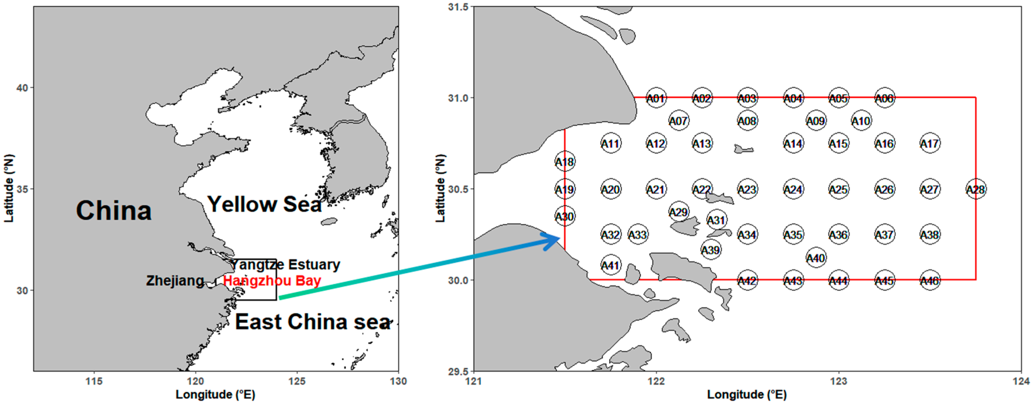
2.1. Study Area and Sampling

The HZB, adjacent to the Yangtze Estuary, is located west of the East China Sea, with an average depth of 8–10 m [20] (Figure 1). It is one of China’s major fishing grounds and is characterized by its complex hydrodynamics [21]. HZB is significantly influenced by the dilution of water from the Yangtze River and the secondary plume of the Yangtze River entering HZB from the north. The tidal range of HZB is about 9 m, which is one of the largest tidal ranges in China [22].
We conducted 7 cruises for fishery resource surveys in April from 2017 to 2023. A total of 46 stations were included on every cruise. We use a bottom trawl to collect small yellow croakers (Figure S1), and the circumference of the tensioned net opening is 25 m. The width of the net opening is 9.9 m, and the mesh size of the cod-end is 2.0 cm. The towing speed at each station is maintained at ~2 knots for 30 min. We also investigated the environmental factors at each station, including depth, temperature, salinity, chlorophyll-a, pH, dissolved oxygen, and turbidity. Environmental data were collected simultaneously with fish sampling. All environmental factors were divided into the surface layer (0–3 m) and the bottom layer according to depth.

2.2. Environmental Variables Selection

In order to prevent overfitting and multi-collinearity issues, we computed the variance inflation factor (VIF) for every candidate predictor variable. Then, we eliminated the redundant predictor variables (those with a VIF value greater than 5) for the construction of subsequent models (Table 1). According to the filtering results, depth (m), sea surface temperature (SST, °C), sea bottom temperature (SBT, °C), sea surface salinity (SSS, PSU), sea bottom salinity (SBS, PSU), sea surface chlorophyll-a (SSChl, mg/m3), sea surface pH (SSPH), sea surface dissolved oxygen (SSO, mg/L), sea bottom dissolved oxygen (SBO, mg/L) and sea surface turbidity (SSTurb) were chosen to construct the species distribution models.

2.3. Data Analyses

The R package biomod2 was used to construct a spatio-temporal distribution model of L. polyactis. This package assembled several frequently used species distribution models. It encompassed classification techniques (such as the generalized boosting model and RF) and regression approaches (such as GLM and GAM). In the context of this research, we chose eleven modeling algorithms. These algorithms included artificial neural networks (ANN), classification tree analysis (CTA), flexible discriminant analysis (FDA), GAM, generalized boosting model (GBM), GLM, multiple adaptive regression splines (MARS), maximum entropy (MaxEnt), RF, surface range envelop (SRE), and XGBOOST [23]. The aim was to uncover the connection between distribution data for species and environmental factors. We randomly split these species distribution data into two components. Out of these data, 70% was applied for the model training process, and 30% was used to evaluate how well the model predicted the results. We use the true skill statistic (TSS) and the receiver operating characteristic (ROC) to evaluate the performances of the algorithms [24,25]. The models were validated using ten-fold cross-validation. Then, we selected the optimal model to predict the habitat of L. polyactis. The values of projected habitat suitability fall between 0 and 1000, where a value of 0 indicates the lowest likelihood of occurrence (i.e., 0), and 1000 stands for the highest likelihood of occurrence (i.e., 1)
We conducted all analyses with R 64-bit (version 4.3.2, 64 bit) software (https://www.r-project.org, accessed on 22 June 2024), using the package “biomod2” for ensemble model construction [23], “raster” for data manipulation [26], and “maps” and “ggplot2” for maps and figures, respectively [27,28].

3. Results

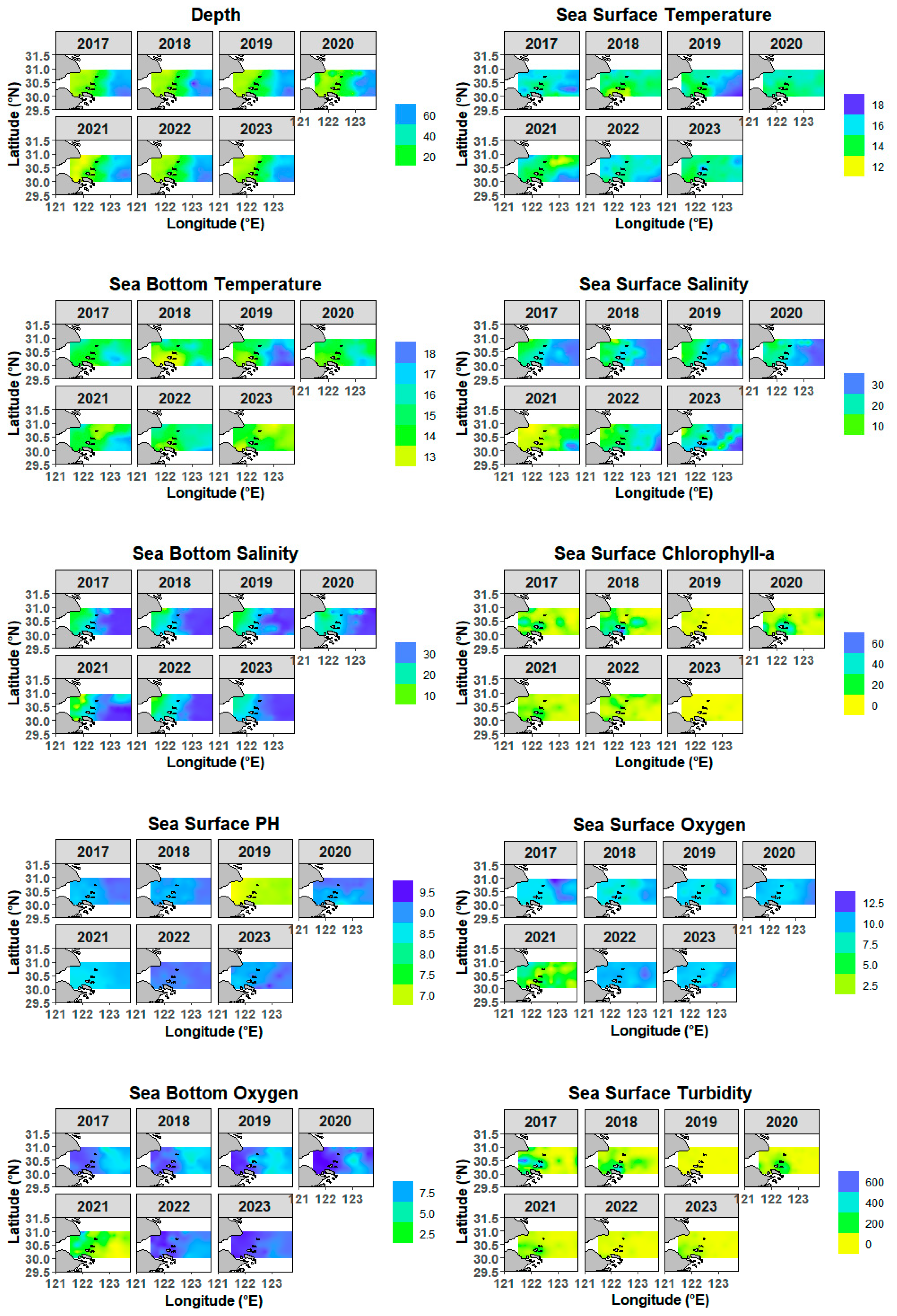
3.1. Characteristics of Environmental Factors

The characteristics of 10 environmental factors were pictured from 2017 to 2023 (Figure 2). An ANOVA test was conducted, showing significant inter-annual variations in SBT, SSS, chlorophyll-a, turbidity, and pH (p < 0.01). The result showed that there was no significant change in depth from 2017 to 2023 (p > 0.05), and it has the characteristic of deepening from the nearshore to the open sea. In 2019, whether it was SST or SBT, extreme values emerged. A high-temperature area appeared in the southeastern region of the study area. On the contrary, the pH value reached a minimum in this year. There is minimal variation in average SBT throughout the years. An extremely low SSS value emerged in 2021, with the range of 3.56–33.66. The dissolved oxygen also showed a decreasing phenomenon in this year. The SSTurb had no significant fluctuation in all seven years.

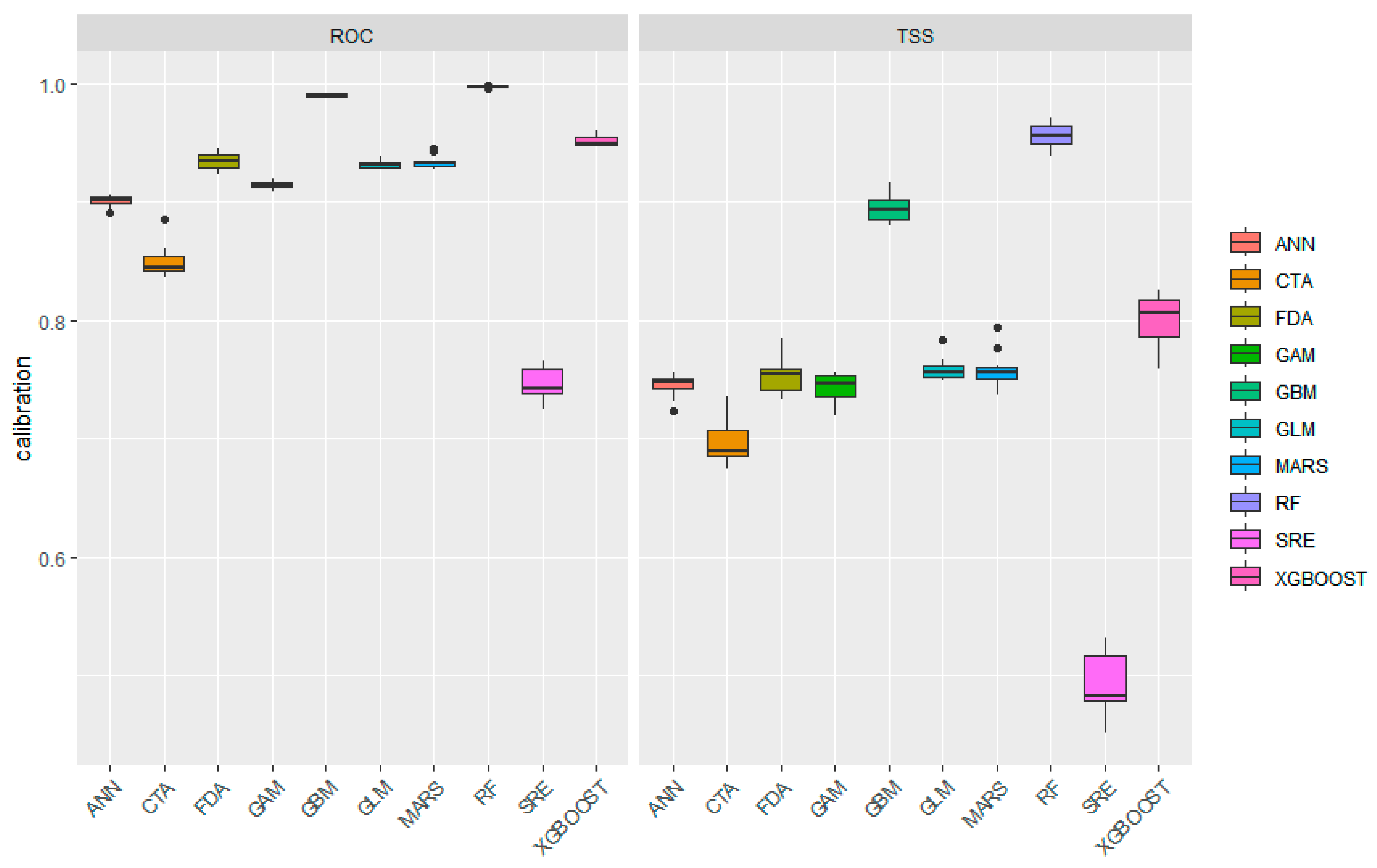
3.2. Model Performance

To evaluate the performance of the 11 algorithms, ROC and TSS values were used for detection (Figure 3). The results showed that the RF algorithm demonstrated the best performance, and the SRE algorithm was the least accurate, with the lowest ROC (around 0.75) and TSS (around 0.5). The GBM algorithm also displayed good performance, being a little inferior to that of RF. The performances of the other algorithms, such as GAM and GLM, are almost the same. The ROC value is around 0.9, and the TSS value is around 0.7. So, we selected the RF algorithms for the subsequent model building. The sensitivity and specificity of the RF model were 95.238 and 99.49, respectively. This showed that the RF model had a more accurate performance.

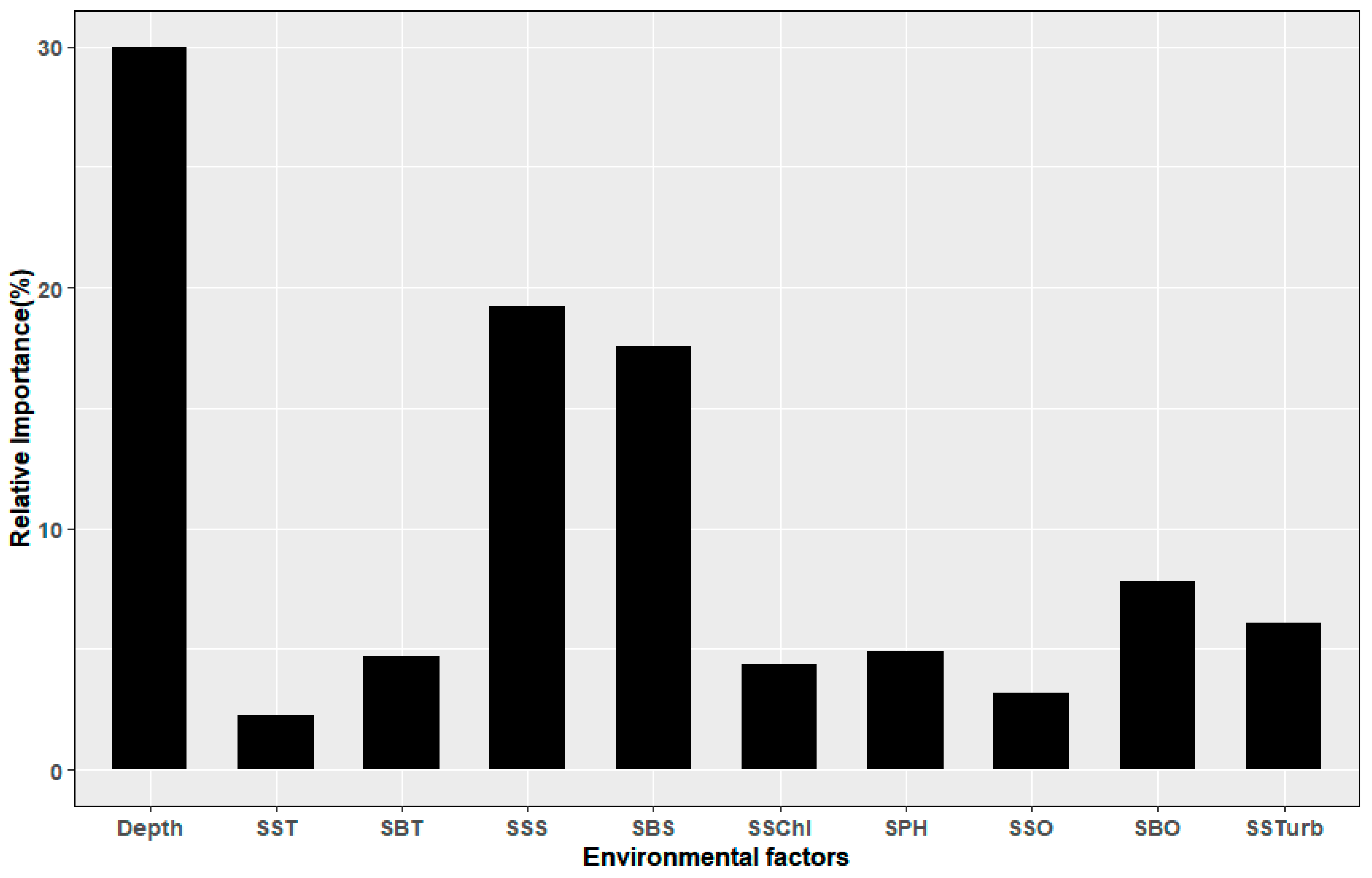
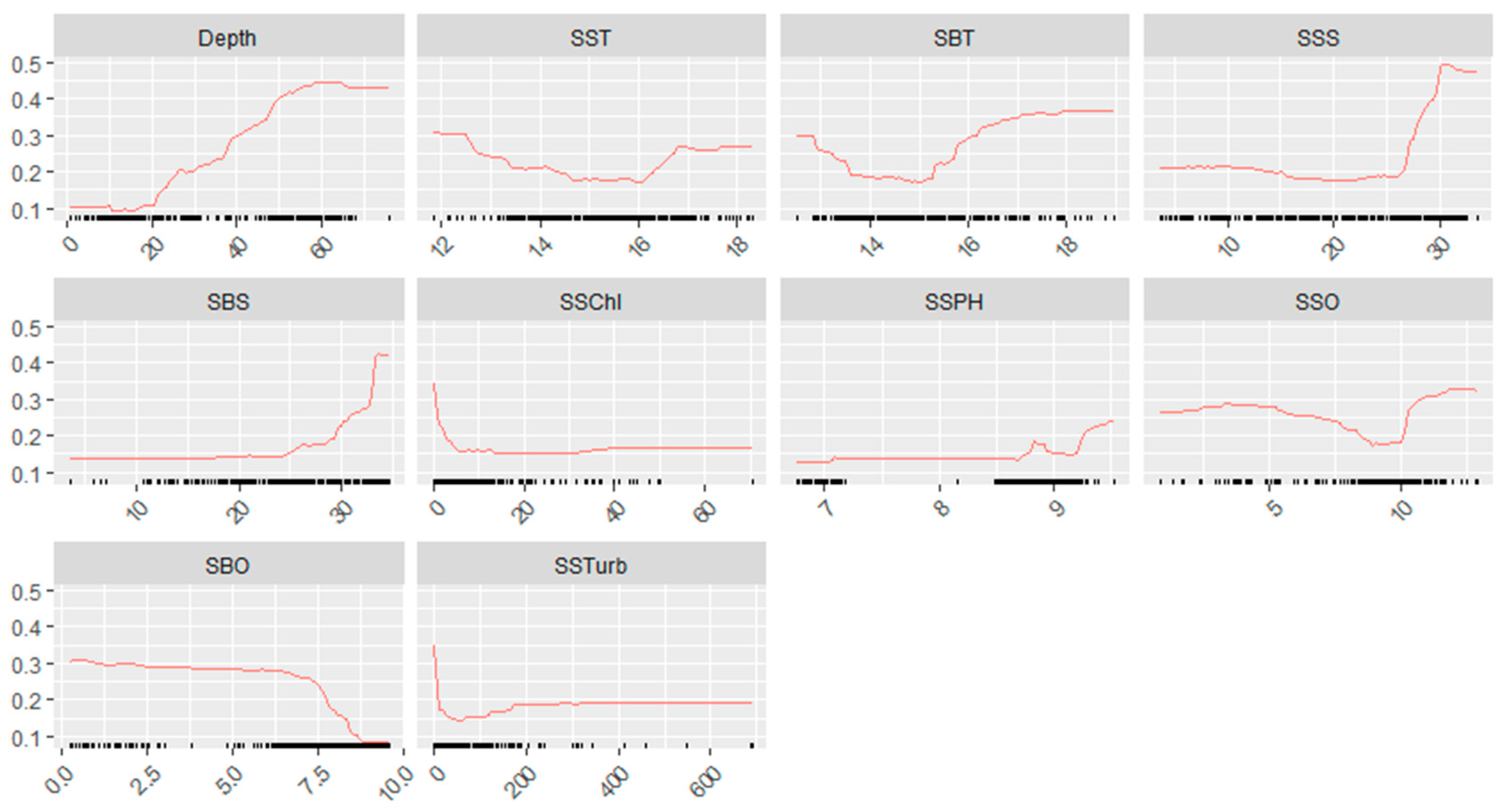
3.3. The Relationship Between L. polyactis Distribution and Environmental Factors

The bar plot showed the relative importance of all ten environmental factors for the distribution of small yellow croakers (Figure 4). Depth was the most important environmental response factor in the model, accounting for 30% of the variation. Salinity was the second most influential factor. Both SSS and SBS had significant impacts on the occurrence probability of small yellow croakers. The combined influence of the remaining seven environmental factors on the distribution is less than 35%. Among the 10 environmental factors, the influence of SST was the lowest on the distribution of small yellow croakers.
The response curve of depth showed that its influence gradually increased from 20 m to 60 m, which meant that the small yellow croakers are mainly found in the deeper water areas (Figure 5), the optimal depth being ~60 m. SSS and SBS showed a similar trend of higher salinity optima, i.e., a non-linear effect on small yellow croaker distribution, with occurrences rare at low salinities. Observations of small yellow croaker occurred in high-salinity areas, especially above 25 PSU. Furthermore, when SBO exceeded 7.5 mg/L, the occurrence of L. polyactis decreased. As for the other factors, due to their relatively low impact on the distribution, it was impossible to identify their appropriate intervals.

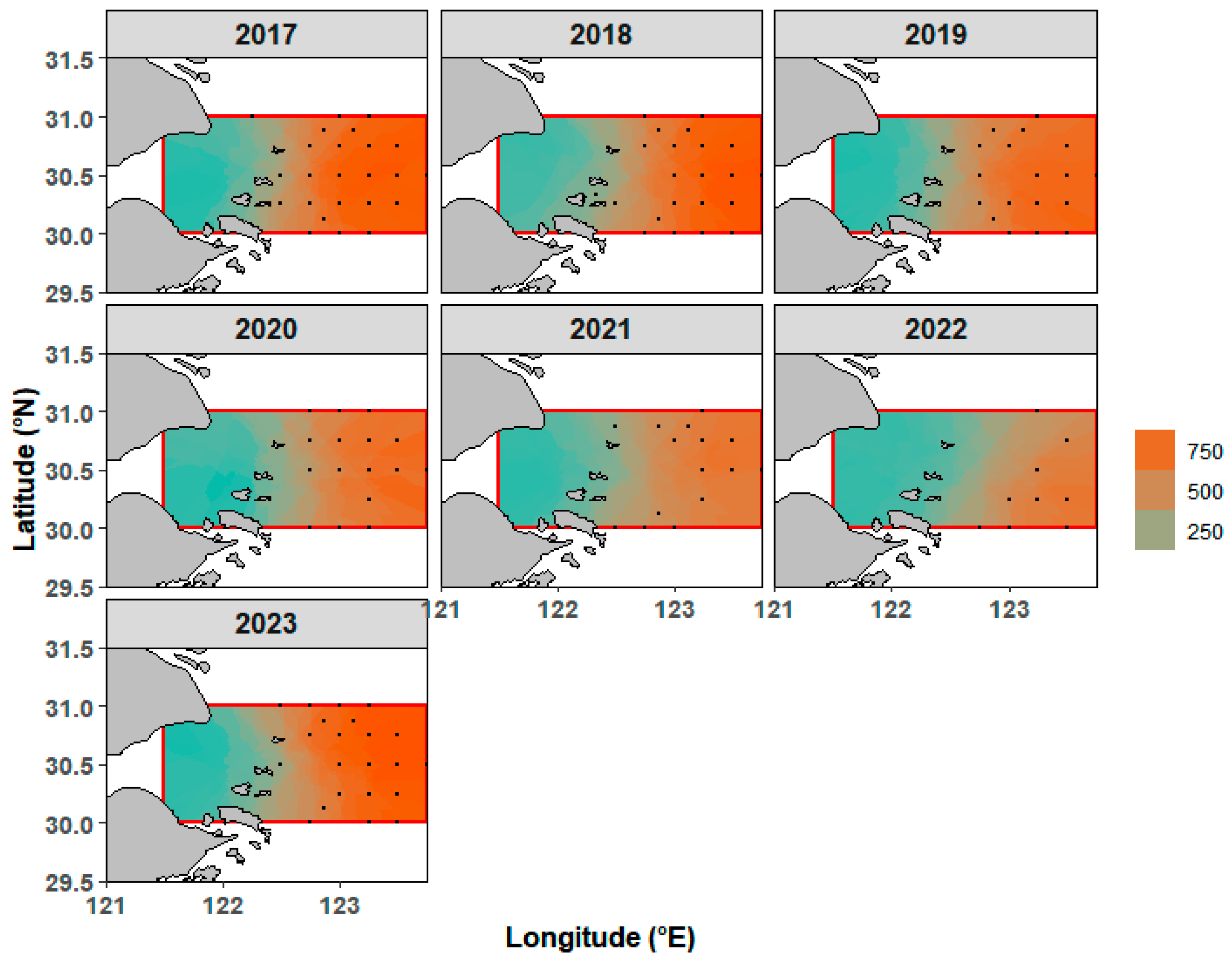
3.4. Spatio-Temporal Distribution of L. polyactis

The number of stations where L. polyactis appeared steadily decreased from 2017 to 2022. The lowest value in 2022 was only nine stations, accounting for 20% of the total stations surveyed. In 2023, the number had rebounded to 22 stations. The predicted present values of L. polyactis were spatially consistent with the observed values (Figure 6), indicating that the spatial distribution pattern of small yellow croakers varied among different years. Generally, the distribution range of small yellow croakers was extensive, mainly found in the offshore regions, particularly in the areas east of 122.5°E. During the years 2021 and 2022, the salinity within the studied area was comparatively low. The regions with high salinity were predominantly located in the southeastern portion of the study area, where small yellow croakers were especially found (Figure 2 and Figure 6).

4. Discussion

4.1. Interpretation of Model Results

In this study, we evaluated the performance of 11 different algorithms for constructing the species distribution model of small yellow croakers. The results clearly demonstrated that the RF algorithm outperformed the others. This superior performance can be attributed to the inherent characteristics of the RF algorithm, which is an ensemble learning method that builds multiple decision trees during training and aggregates their predictions [29,30]. RF is particularly effective in handling large datasets with numerous predictor variables, and it is robust to noise and outliers, making it suitable for complex ecological data [31,32,33]. Numerous studies have shown that the RF model performs better than traditional linear models under completely unknown circumstances [29,34]. Moreover, the performance of the RF model depends on the appropriate selection of hyperparameters and variables, which is also useful for simplifying the model and avoiding overfitting problems [32]. The RF model, despite its better predictive power, suffers from inherent limitations such as its black-box nature, interpretability challenges due to complex ensemble decision-making, high computational overhead, sensitivity to imbalanced data and outliers, and potential overfitting in certain scenarios [34].
Similar performances of algorithms such as GAM and GLM indicate that they have limitations in capturing the complex non-linear relationships between small yellow croaker distributions and environmental factors [29]. The ROC value of 0.9 and TSS value of 0.7 for these models suggest that they can provide a basic level of prediction but are not as accurate as the more advanced machine learning algorithms. These traditional species distribution models have advantages in model fitting [35,36]. However, good data fitting and a high explanatory power of the model do not necessarily guarantee good predictive performance of the model [34]. The relatively poor performance of the SRE algorithm suggests that simplistic models based on environmental envelopes are inadequate for predicting species distribution in highly changing environments, such as HZB. The SRE algorithm depends on the range of environmental conditions where a species is found, but it does not consider how different environmental factors interact, which reduces its accuracy [11,37]. In contrast, the RF model’s ability to handle complex interactions and its robustness to overfitting make it a more reliable tool for predicting the distribution of small yellow croakers [38].

4.2. Environmental Variable Predictors

The ecological characteristics of a fish species are closely related to their preference for specific environmental conditions, which is critical for understanding habitat selection [7,39,40]. In this study, depth is the most influential environmental factor, accounting for 30% of the importance in the model. Depth can affect factors such as temperature and pressure, thereby affecting the living habits and abundance patterns of fish. Therefore, water depth indirectly affects the spatial distribution of small yellow croakers by influencing factors such as temperature and salinity factors. The response curve indicated that the influence of depth increased gradually from 20 to 60 m, with the optimal depth for the small yellow croaker distribution being ~60 m. This suggests that small yellow croaker prefers deeper waters, where environmental conditions such as temperature and salinity are more stable [41,42]. Deeper waters may also provide a refuge from predation and human disturbances, making them more suitable habitats for this species [43]. Salinity, both SSS and SBS, was the second most important factor influencing the distribution of small yellow croakers. The curvilinear effect of salinity on species distribution indicates that small yellow croakers are much less likely to occur in low-salinity areas, in contrast to areas where salinity exceeds 25 PSU. The result is consistent with previous research findings [3]. Salinity plays a critical role in the osmoregulation of fish, and the small yellow croaker likely adapted to particular salinity ranges, allowing it to survive effectively. The findings from relevant studies on similar salinity adaptations provide strong support for this hypothesis [41]. Additionally, salinity fluctuations can impact the availability of prey organisms and the overall ecological balance, further influencing the distribution of this species [44].
The combined influence of the remaining seven environmental factors (SST, SBT, SSChl, sea SSPH, SSO, SBO, and SSTurb) was less than 35%. Among these, SST had the lowest impact on the distribution of small yellow croakers, which contrasts with findings from other studies where temperature is a dominant factor [45]. The low SST impact may be attributed to this study’s narrow thermal range, which is the optimal temperature for small yellow croaker activity. This discrepancy may be due to the unique hydrodynamics of HZB, where other factors, such as salinity and depth, play more significant roles in shaping the habitat of small yellow croakers. The relatively low impact of SST could also be attributed to the buffering effect of the complex water masses and mixing processes in the bay, which may mitigate the influence of temperature fluctuations on species distribution. Moreover, we guess that hyperoxic conditions (>7.5 mg/L) may induce oxidative stress or alter prey distribution, which requires further study.

4.3. Spatio-Temporal Dynamics

This investigation into the distribution pattern of small yellow croakers should facilitate an understanding of how fish select their habitats in estuaries, uncovering the relevant mechanisms. The spatio-temporal distribution of small yellow croakers in HZB exhibited significant changes from 2017 to 2023. The number of stations where small yellow croakers were observed steadily decreased from 2017 to 2022, down to just nine stations (20% of the total stations surveyed). However, in 2023, the number of stations with a small yellow croaker presence rebounded to 22. The 2023 recovery may be linked to both environmental improvements (salinity normalization) and the 2022 fishing ban. This pattern suggests a combination of anthropogenic and environmental factors influencing the dynamics of this species [46]. The relatively low salinity of 2021–2022, which may be caused by higher Yangtze River discharge during those wet seasons, may have reduced environmental suitability for small yellow croaker, contracting their distribution range. Moreover, spring is the spawning season for small yellow croakers, and its distribution is primarily influenced by reproductive requirements and the feeding needs of juvenile fish [47]. In April, small yellow croakers migrate to the spawning ground protection area of the Zhoushan fishing ground (in the offshore waters of HZB) and its surrounding waters for spawning or feeding [21]. After the establishment of the spawning ground protection area in 2017, a complete fishing ban has been enforced since April. The protection measures in the spawning ground area began one month earlier than the nationwide summer fishing moratorium, which may have contributed to protecting the spawning adults of the small yellow croaker.
Spatially, small yellow croakers were predominantly distributed in the offshore regions of HZB, particularly in areas east of 122.5° E. This distribution pattern aligns with the influence of key environmental factors, such as depth and salinity. Offshore areas, being deeper and saltier, are preferred by small yellow croakers and higher salinity levels, which are more favorable for their survival. The southeastern portion of the study area, characterized by high salinity, was particularly important for the small yellow croaker distribution during years when the salinity levels in other parts of the bay were less suitable.

4.4. Implications for Conservation and Management

Understanding the spatio-temporal dynamics of the small yellow croaker distribution in HZB is crucial for the sustainable management of this ecologically and economically important species. The findings of this study highlight the importance of depth and salinity as key environmental factors influencing the distribution of small yellow croakers. Conservation efforts should focus on protecting deep-water habitats and maintaining suitable salinity conditions to support the recovery and sustainability of small yellow croaker populations. The implementation of marine protected areas (MPAs) in regions with optimal environmental conditions, such as the southeastern offshore areas of HZB, could provide nursery refuge for small yellow croakers and other commercially important species [7,48,49]. For example, designating MPAs in high-salinity (25–30 PSU) zones and implementing seasonal closures during spawning (April-May) are useful for this croaker population. If MPAs or seasonal closures are expanded, short-term catches will face a reduction, which will have a certain impact on the fishery economy. The rebound in small-bodied yellow croaker populations in 2023, following the expansion of spawning ground protections, highlights the potential for targeted habitat restoration and potential spillover benefits outside MPAs [47,50]. Seasonal fishing closures during critical periods, such as spawning seasons in April, could also help protect juvenile and adult fish and allow the population to recover [21].

5. Conclusions

In conclusion, this study provides a comprehensive understanding of the spatio-temporal dynamics of small yellow croakers in HZB and highlights the importance of integrating environmental factors into species distribution models. The findings underscore the need for targeted conservation and management strategies to protect this valuable species and ensure the health of marine ecosystems in the region. These findings provide a framework for managing fish populations in eutrophic coastal ecosystems across East Asia, including the Yellow Sea and the Bohai Sea. Future research could integrate climate change projections and fine-scale fishing effort data to refine conservation strategies under changing environmental conditions. Such protective strategies should also apply to North America [50], including colder, less eutrophic seawaters that Pacific salmon need to thrive [51].

Supplementary Materials

The following supporting information can be downloaded at: https://www.mdpi.com/article/10.3390/fishes10060298/s1, Figure S1: Schematic diagram of small yellow croaker (Larimichthys polyactis).

Author Contributions

Conceptualization, R.J. and Y.Z.; methodology, D.W.; data curation, M.H.; writing—original draft preparation, X.L. and P.S.; writing—review and editing, P.S. All authors have read and agreed to the published version of the manuscript.

Funding

This study was supported by the National Key R&D Program (2024YFD2400402) and the Zhejiang Marine Fisheries Research Institute Science and Technology Program (HYS-ZX-202307).

Institutional Review Board Statement

This research focuses on the ecological study of wild fish habitats (small yellow croaker, Larimichthys polyactis) through fisheries surveys and modeling, which involves no human subjects, vertebrate animal experiments, or protected species. All data were collected through non-invasive marine ecological surveys compliant with Chinese regulations for fishery resource research. No Ethics Approval is required, as the study does not involve sensitive biological materials, human participants, or animal welfare concerns.

Informed Consent Statement

Not applicable.

Data Availability Statement

Data are unavailable because of institutional access restrictions. Contact the corresponding author for data requests.

Acknowledgments

We thank our colleagues for their contributions to data collection and laboratory experiments. Comments by anonymous reviewers on earlier versions helped improve the manuscript.

Conflicts of Interest

The authors declare that they have no known competing financial interests or personal relationships that could have appeared to influence the work reported in this paper.

References

  1. Lin, L.S.; Liu, Z.L.; Jiang, Y.Z.; Huang, W.; Gao, T.X. Current status of small yellow croaker resources in the southern Yellow Sea and the East China Sea. Chin. J. Oceanol. Limnol. 2011, 29, 547–555. [Google Scholar] [CrossRef]
  2. Zhang, C.; Ye, Z.J.; Wan, R.; Ma, Q.Y.; Li, Z.G. Investigating the population structure of small yellow croaker (Larimichthys polyactis) using internal and external features of otoliths. Fish. Res. 2014, 153, 41–47. [Google Scholar] [CrossRef]
  3. Xu, M.; Wang, Y.H.; Liu, Z.L.; Liu, Y.; Zhang, Y.; Yang, L.L.; Wang, F.; Wu, H.; Cheng, J.H. Seasonal distribution of the early life stages of the small yellow croaker (Larimichthys polyactis) and its dynamic controls adjacent to the Changjiang River Estuary. Fish. Oceanogr. 2023, 32, 390–404. [Google Scholar] [CrossRef]
  4. Ma, Q.; Yan, J.; Ren, Y. Linear mixed-effects models to describe length-weight relationships for yellow croaker (Larimichthys polyactis) along the north coast of China. PLoS ONE 2017, 12, e0171811. [Google Scholar] [CrossRef]
  5. Zheng, J.; Gao, T.X.; Yan, Y.R.; Song, N. Genetic variation of the small yellow croaker (Larimichthys polyactis) inferred from mitochondrial DNA provides novel insight into the fluctuation of resources. Acta Oceanol. Sin. 2022, 41, 88–95. [Google Scholar] [CrossRef]
  6. Tang, Y.L.; Ma, S.Y.; Liu, C.D.; Wang, X.; Cheng, S. Influence of spatial-temporal and environmental factors on Larimichthys polyactis, Octopus variabilis, and species aggregated set-net CPUEs in Haizhou Bay, China. J. Ocean Univ. China 2018, 17, 973–982. [Google Scholar] [CrossRef]
  7. Rubec, P.J.; Santi, C.E.; Ault, J.S.; Monaco, M.E. Development of modelling and mapping methods to predict spatial distributions and abundance of estuarine and coastal fish species life-stages in Florida. Aquac. Fish Fish. 2023, 3, 1–22. [Google Scholar] [CrossRef]
  8. Barletta, M.; Barletta-Bergan, A.; Saint-Paul, U.; Hubold, G. The role of salinity in structuring the fish assemblages in a tropical estuary. J. Fish Bio. 2005, 66, 45–72. [Google Scholar] [CrossRef]
  9. Elliott, M.; Whitfield, A.K. Challenging paradigms in estuarine ecology and management. Estuar. Coast. Shelf Sci. 2011, 94, 306–314. [Google Scholar] [CrossRef]
  10. Sun, Y.Y.; Zhang, H.; Jiang, K.J.; Xiang, D.L.; Shi, Y.C.; Huang, S.S.; Li, Y.; Han, H.B. Simulating the changes of the habitats suitability of chub mackerel (Scomber japonicus) in the high seas of the North Pacific Ocean using ensemble models under medium to long-term future climate scenarios. Mar. Pollut. Bull. 2024, 207, 12. [Google Scholar] [CrossRef]
  11. Song, X.; Hu, F.; Xu, M.; Zhang, Y.; Jin, Y.; Gao, X.; Liu, Z.; Ling, J.; Li, S.; Cheng, J. Spatiotemporal distribution and dispersal pattern of early life stages of the small yellow croaker (Larimichthys polyactis) in the southern Yellow Sea. Diversity 2024, 16, 521. [Google Scholar] [CrossRef]
  12. Yin, J.; Wang, J.; Zhang, C.L.; Xu, B.D.; Xue, Y.; Ren, Y.P. Spatial and temporal distribution characteristics of Larimichthys polyactis eggs in Haizhou Bay and adjacent regions based on two- stage GAM. J. Fish. Sci. China 2019, 26, 1164–1174. [Google Scholar]
  13. Wan, R.; Song, P.; Li, Z.; Long, X.; Wang, D.; Zhai, L. Use of ensemble model for modeling the larval fish habitats of different ecological guilds in the Yangtze Estuary. Fishes 2023, 8, 209. [Google Scholar] [CrossRef]
  14. Brunel, T.; van Damme, C.J.G.; Samson, M.; Dickey-Collas, M. Quantifying the influence of geography and environment on the northeast Atlantic mackerel spawning distribution. Fish. Oceanogr. 2017, 27, 159–173. [Google Scholar] [CrossRef]
  15. Li, M.; Wang, B.; Li, Y. Influence of suspended particulate matters on P dynamics and eutrophication in the highly turbid estuary: A case study in Hangzhou Bay, China. Mar. Pollut. Bull. 2024, 207, 116793. [Google Scholar] [CrossRef]
  16. Longhurst, A.R.; Harrison, W.G. The biological pump: Profiles of plankton production and consumption in the upper ocean. Prog. Oceanogr. 1989, 22, 47–123. [Google Scholar] [CrossRef]
  17. Jin, Z.H.; Xu, K.D.; Zhang, H.L.; Zhou, Y.D.; Long, X.Y.; Zhan, W.; Ma, W.J.; Xu, F. Resource assessment of the near-shore Sciaenidae fishes in Zhejiang Province, China. J. Dalian Fish. Univ. 2025, 1–16. [Google Scholar]
  18. Lu, Z.H.; Miao, Z.Q.; Lin, N. The structure and diversity fish communities in Spring in the middle sea area of Zhejiang Province and adjacent region. J. Zhejiang Ocean Univ. 2009, 28, 51–56. [Google Scholar]
  19. Ren, J.S.; Jin, X.S.; Yang, T.; Kooijman, S.A.L.M.; Shan, X.J. A dynamic energy budget model for small yellow croaker Larimichthys polyactis: Parameterisation and application in its main geographic distribution waters. Ecol. Model. 2020, 427, 109051. [Google Scholar] [CrossRef]
  20. Rao, W.B.; Mao, C.P.; Wang, Y.G.; Su, J.B.; Balsam, W.; Ji, J.F. Geochemical constraints on the provenance of surface sediments of radial sand ridges off the Jiangsu coastal zone, East China. Mar. Geol. 2015, 359, 35–49. [Google Scholar] [CrossRef]
  21. Liu, Z.L.; Jin, Y.; Yang, L.L.; Yan, L.P.; Zhang, Y.; Xu, M.; Tang, J.H.; Zhou, Y.D.; Hu, F.; Cheng, J.H. Incorporating egg-transporting pathways into conservation plans of spawning areas: An example of small yellow croaker (Larimichthys polyactis) in the East China Sea zone. Front. Mar. Sci. 2022, 9, 941411. [Google Scholar] [CrossRef]
  22. Zhou, F.; Su, J.L.; Huang, D.J. Study on the intrusion of coastal low salinity water in the west of southern Huanghai Sea during spring and summer. Haiyang Xuebao 2004, 26, 34–44. [Google Scholar]
  23. Thuiller, W.; Georges, D.; Engler, R.; Breiner, F. biomod2: Ensemble Platform for Species Distribution Modeling; R Package: Vienna, Austria, 2016; Available online: https://CRAN.R-project.org/package=biomod2 (accessed on 1 January 2020).
  24. Allouche, O.; Tsoar, A.; Kadmon, R. Assessing the accuracy of species distribution models: Prevalence, kappa and the true skill statistic (TSS). J. Appl. Ecol. 2006, 43, 1223–1232. [Google Scholar] [CrossRef]
  25. Wang, Y.S.; Xie, B.Y.; Wan, F.H.; Xiao, Q.M.; Dai, L.Y. Application of ROC curve analysis in evaluating the performance of alien species’ potential distribution models. Biodivers. Sci. 2007, 4, 365–372. (In Chinese) [Google Scholar]
  26. Hijmans, R.J. Raster: Geographic Data Analysis and Modeling; R Package: Vienna, Austria, 2014; Available online: http://CRAN.Rproject.org/package=raster (accessed on 1 January 2020).
  27. Deckmyn, A. Maps: Draw Geographical Maps; R Package: Vienna, Austria, 2022; Available online: http://CRAN.R-project.org/package=maps (accessed on 1 January 2020).
  28. Ginestet, C. ggplot2: Elegant Graphics for Data Analysis. J. R. Stat. Soc. 2011, 174, 245–246. [Google Scholar] [CrossRef]
  29. Li, Z.G.; Ye, Z.J.; Wan, R.; Zhang, C. Model selection between traditional and popular methods for standardizing catch rates of target species: A case study of Japanese Spanish mackerel in the gillnet fishery. Fish. Res. 2015, 161, 312–319. [Google Scholar] [CrossRef]
  30. Lee-Yaw, J.A.; McCune, J.L.; Pironon, S. Species distribution models rarely predict the biology of real populations. Ecography 2022, 2022, e05877. [Google Scholar] [CrossRef]
  31. Savage, S.L.; Lawrence, R.L.; Squires, J.R. Predicting relative species composition within mixed conifer forest pixels using zero-inflated models and Landsat imagery. Remote Sens. Environ. 2015, 171, 326–336. [Google Scholar] [CrossRef]
  32. de la Hoz, C.F.; Ramos, E.; Puente, A.; Juanes, J.A. Temporal transferability of marine distribution models: The role of algorithm selection. Ecol. Indic. 2019, 106, 105499.1–105499.14. [Google Scholar] [CrossRef]
  33. Li, M.; Zhang, C.L.; Xu, B.D. Evaluating the approaches of habitat suitability modelling for whitespotted conger (Conger myriaste). Fish. Res. 2017, 195, 230–237. [Google Scholar] [CrossRef]
  34. Li, Z.G.; Wan, R.; Ye, Z.J.; Chen, Y.; Ren, Y.P.; Liu, H.; Jiang, Y.Q. Use of random forests and support vector machines to improve annual egg production estimation. Fish. Sci. 2017, 83, 1–11. [Google Scholar] [CrossRef]
  35. Murase, H.; Nagashima, H.; Yonezaki, H.; Matsukura, R.; Kitakado, T. Application of a generalized additive model (GAM) to reveal relationships between environmental factors and distributions of pelagic fish and krill: A case study in Sendai Bay, Japan. ICES J. Mar. Sci. 2009, 66, 1073–1080. [Google Scholar] [CrossRef]
  36. Akter, S.; Abhilash, W.K.; Nama, S.; Borah, S.; Angmo, S.; Deshmukhe, G.; Nayak, B.B.; Ramteke, K. Phytoplankton-environment dynamics in a tropical estuary of the northeastern Arabian Sea: A Generalized Additive Model (GAM) approach. Environ. Monit. Assess. 2025, 197, 201. [Google Scholar] [CrossRef] [PubMed]
  37. Yang, T.Y.; Liu, X.Y.; Han, Z.Q. Predicting the effects of climate change on the suitable habitat of Japanese Spanish Mackerel (Scomberomorus niphonius) based on the species distribution model. Front. Mar. Sci. 2022, 9, 927790. [Google Scholar] [CrossRef]
  38. Pang, H.; Lin, A.P.; Holford, M.; Enerson, B.E.; Lu, B.; Lawton, M.P.; Floyd, E.; Zhao, H. Pathway analysis using random forests classification and regression. Bioinformatics 2006, 22, 2028–2036. [Google Scholar] [CrossRef]
  39. Potter, I.C.; Tweedley, J.R.; Elliott, M.; Whitfield, A.K. The ways in which fish use estuaries: A refinement and expansion of the guild approach. Fish Fish. 2015, 16, 230–239. [Google Scholar] [CrossRef]
  40. Bento, E.G.; Grilo, T.F.; Nyitrai, D.; Dolbeth, M.; Pardal, M.A.; Martinho, F. Climate influence on juvenile European sea bass (Dicentrarchus labrax, L.) populations in an estuarine nursery: A decadal overview. Mar. Environ. Res. 2016, 122, 93–104. [Google Scholar] [CrossRef]
  41. Ding, F.Y.; Lin, L.S.; Li, J.S.; Cheng, J.H. Distribution of the spawning population of small yellow croaker (Larimichthys polyactis) in the northern East China Sea and its relationship with water masses. J. Nat. Resour. 2007, 22, 1013–1019. (In Chinese) [Google Scholar]
  42. Galaiduk, R.; Radford, B.T.; Saunders, B.J.; Newman, S.J.; Harvey, E.S. Characterizing ontogenetic habitat shifts in marine fishes: Advancing nascent methods for marine spatial management. Ecol. Appl. 2017, 27, 1776–1788. [Google Scholar] [CrossRef]
  43. Parsons, D.F.; Suthers, I.M.; Cruz, D.O.; Smith, J.A. Effects of habitat on fish abundance and species composition on temperate rocky reefs. Mar. Ecol. Prog. Ser. 2016, 561, 155–171. [Google Scholar] [CrossRef]
  44. Dambrine, C.; Woillez, M.; Huret, M.; de Pontual, H. Characterising Essential Fish Habitat using spatio-temporal analysis of fishery data: A case study of the European seabass spawning areas. Fish. Oceanogr. 2021, 30, 413–428. [Google Scholar] [CrossRef]
  45. Zhong, X.M.; Zhang, H.; Tang, J.H.; Zhong, F.; Zhong, J.S.; Xiong, Y.; Gao, Y.S.; Ge, K.K.; Yu, W.W. Temporal and spatial distribution of Larimichthys polyactis Bleeker resources in offshore areas of Jiangsu Province. J. Fish. China 2011, 235, 238–246. [Google Scholar]
  46. Lin, N.; Chen, Y.G.; Jin, Y.; Yuan, X.W.; Ling, J.Z.; Jiang, Y.Z. Distribution of the early life stages of small yellow croaker in the Yangtze River estuary and adjacent waters. Fish. Sci. 2018, 84, 357–363. [Google Scholar] [CrossRef]
  47. Wang, Y.L.; Hu, C.L.; Xu, K.D.; Zhou, Y.D.; Jiang, R.J.; Li, Z.H.; Li, X.F. Reproductive status of Larimichthys polyactis in Zhoushan fishing ground and adjacent waters from 2020 to 2021. Ocean Dev. Manag. 2022, 39, 53–57. [Google Scholar]
  48. Benedetti-Cecchi, L.; Bertocci, I.; Micheli, F.; Maggi, E.; Fosella, T.; Vaselli, S. Implications of spatial heterogeneity for management of marine protected areas (MPAs): Examples from assemblages of rocky coasts in the northwest Mediterranean. Mar. Environ. Res. 2003, 55, 429–458. [Google Scholar] [CrossRef]
  49. Garcia-Charton, J.A.; Perez-Ruzafa, A.; Marcos, C.; Claudet, J.; Badalamenti, F.; Benedetti-Cecchi, L.; Falcón, J.M.; Milazzo, M.; Schembri, P.J.; Stobart, B.; et al. Effectiveness of European Atlanto-Mediterranean MPAs: Do they accomplish the expected effects on populations, communities and ecosystems? J. Nat. Conserv. 2008, 16, 193–221. [Google Scholar] [CrossRef]
  50. Roberts, C.M.; Bohnsack, J.A.; Gell, F.; Hawkins, J.P.; Goodridge, R. Effects of marine reserves on adjacent fisheries. Science 2001, 294, 1920–1923. [Google Scholar] [CrossRef]
  51. Greenberg, P. Four Fish: The Future of the Last Wild Food; Penguin: New York, NY, USA, 2010; 285p. [Google Scholar]
Figure 1. Survey stations in the coastal waters of Hangzhou Bay.
Fishes 10 00298 g001
Figure 2. Characteristics of ten environmental factors (depth (m), sea surface temperature (SST, °C), sea bottom temperature (SBT, °C), sea surface salinity (SSS, PSU), sea bottom salinity (SBS, PSU), sea surface chlorophyll-a (SSChl, mg/m3), sea surface pH (SSPH), sea surface dissolved oxygen (SSO, mg/L), sea bottom dissolved oxygen (SBO, mg/L), and sea surface turbidity (SSTurb, NTU)) between 2017 and 2023 in the HZB.
Fishes 10 00298 g002
Figure 3. Model performance of eleven algorithms (artificial neural networks (ANN), classification tree analysis (CTA), flexible discriminant analysis (FDA), generalized additive model (GAM), generalized boosting model (GBM), generalized linear model (GLM), multiple adaptive regression splines (MARS), maximum entropy (MaxEnt), random forest (RF), surface range envelop (SRE), and extreme gradient boosting training (XGBOOST)) by using the true skill statistic (TSS) and the receiver operating characteristic (ROC).
Fishes 10 00298 g003
Figure 4. Relative importance of environmental factors (depth (m), sea surface temperature (SST, °C), sea bottom temperature (SBT, °C), sea surface salinity (SSS, PSU), sea bottom salinity (SBS, PSU), sea surface chlorophyll-a (SSChl, mg/m3), sea surface pH (SSPH), sea surface dissolved oxygen (SSO, mg/L), sea bottom dissolved oxygen (SBO, mg/L), and sea surface turbidity (SSTurb)) on the distribution of L. polyactis.
Fishes 10 00298 g004
Figure 5. Response curves of ten environmental factors (depth (m), sea surface temperature (SST, °C), sea bottom temperature (SBT, °C), sea surface salinity (SSS, PSU), sea bottom salinity (SBS, PSU), sea surface chlorophyll-a (SSChl, mg/m3), sea surface pH (SSPH), sea surface dissolved oxygen (SSO, mg/L), sea bottom dissolved oxygen (SBO, mg/L), and sea surface turbidity (SSTurb)) for L. polyactis in the HZB.
Fishes 10 00298 g005
Figure 6. Potential distribution of L. polyactis in the HZB. Points represented the survey values, and colors represented the model-predicted values.
Fishes 10 00298 g006
Table 1. Variable selection for subsequent model building.
VariableDepthSSTSBTSSSSBSSSChlSBChlSSPHSBPHSSOSBOSSTurbSBTurb
Before filtering4.592.342.902.973.853.785.9447.2546.933.834.253.516.34
After filtering4.142.272.812.803.732.61/1.24/3.584.122.59/
Disclaimer/Publisher’s Note: The statements, opinions and data contained in all publications are solely those of the individual author(s) and contributor(s) and not of MDPI and/or the editor(s). MDPI and/or the editor(s) disclaim responsibility for any injury to people or property resulting from any ideas, methods, instructions or products referred to in the content.

