Article

Parallel Privacy-Preserving Shortest Path Algorithms

1
Institute of Computer Science, University of Tartu, Narva Mnt. 18, 51009 Tartu, Estonia
2
Cybernetica AS, Mäealuse 2/1, 12618 Tallinn, Estonia
*
Author to whom correspondence should be addressed.
Cryptography 2021, 5(4), 27; https://doi.org/10.3390/cryptography5040027
Submission received: 14 August 2021 / Revised: 20 September 2021 / Accepted: 7 October 2021 / Published: 14 October 2021

Abstract

:
In this paper, we propose and present secure multiparty computation (SMC) protocols for single-source shortest distance (SSSD) and all-pairs shortest distance (APSD) in sparse and dense graphs. Our protocols follow the structure of classical algorithms—Bellman–Ford and Dijkstra for SSSD; Johnson, Floyd–Warshall, and transitive closure for APSD. As the computational platforms offered by SMC protocol sets have performance profiles that differ from typical processors, we had to perform extensive changes to the structure (including their control flow and memory accesses) and the details of these algorithms in order to obtain good performance. We implemented our protocols on top of the secret sharing based protocol set offered by the Sharemind SMC platform, using single-instruction-multiple-data (SIMD) operations as much as possible to reduce the round complexity. We benchmarked our protocols under several different parameters for network performance and compared our performance figures against each other and with ones reported previously.

1. Introduction

A path from one vertex to another vertex in an edge-weighted directed graph is a sequence of edges, where the starting vertex of each edge is the ending vertex of the previous edge; the first edge starts at the first vertex, and the last edge ends at the second vertex. The length of a path is the sum of the weights of the edges in it. A path from one vertex to another one is shortest if its length is the minimum over all paths between these vertices. The all-pairs shortest distance (APSD) task for a graph is to find the lengths of the shortest paths from any vertex to any other vertex of this graph. The task of Single-Source Shortest Distances (SSSD) for a graph, and a vertex in it is to find the lengths of the shortest paths from the given vertex to all vertices. The shortest path algorithms in graphs are widely used in various fields in computer networks, traffic simulations, bioinformatics, and other computations. They have also been researched in settings where privacy constraints are important [1], typically with different parties holding the descriptions of different parts of the graph.
Secure multiparty computation (SMC) [2,3,4] is a well-known privacy-enhancing technology. Given the description of a function with n inputs and outputs, a SMC protocol for n parties allows each of these parties to supply one input to the function, and learn one of the outputs, such that no party or a tolerated coalition of parties learns anything besides their own outputs. SMC is a universal method, supporting any computable function; hence, the SMC protocols are expensive computationally and/or in their bandwidth usage.
SMC protocols typically expect the function to be represented as an arithmetic or a boolean circuit. This contrasts with the typical representations of programs (algorithms), which have control flow, and use memory, which is read and written at addresses computed during the algorithm execution. All of these features can be translated to circuits, but with significant overheads [5]. Moreover, secret sharing [6] based SMC protocol sets [3], which can be the most efficient ones for large-scale privacy-preserving computations, have significant latency for each operation due to the required interaction between parties (except for homomorphic operations concerning the used secret-sharing scheme). Hence, this efficiency only materializes for highly parallel tasks.
The usual approach to privacy-preserving SSSD and APSD is the implementation of “standard” algorithms [7] on top of some SMC protocol set, with the partition of input data among several parties handled through the standard means of this protocol set. However, such approach for privacy-preserving SSSD is made more complex by several aspects of both the problem itself, as well as the typical algorithms one might want to adapt to run on top of an SMC protocol set. First, the data access patterns and possibly the algorithm’s control flow heavily depend on the lengths of the edges. Neither of these are natively protected by any SMC protocol set. To implement the standard algorithms on top of a SMC protocol set, either the unsupported dependencies have to be removed from the algorithm, or the computations containing them must be emulated, with significant overheads that depend on the used protocol set. Second, SSSD algorithms have been proven hard to parallelize efficiently.
Nevertheless, this approach to privacy-preserving SSSD has been realized by Aly et al. [8,9], who gave implementations of Bellman–Ford and Dijkstra algorithms following this paradigm. After expanding the underlying SMC protocol set with subroutines for oblivious RAM [10], thereby obtaining support for private data dependent memory access, the same paradigm was followed by Keller and Scholl [11] for the Bellman–Ford algorithm and Liu et al. [12] for Dijkstra’s algorithm, albeit with the overheads associated with SMC protocols for oblivious RAM.
Our hypothesis is that privacy-preserving SSSD and APSD algorithms may indeed be constructed using this paradigm of implementing standard SSSD and APSD algorithms on top of some SMC protocol set. However, in order to maximize performance, the implementation cannot be a simple composition of free-standing privacy-preserving subroutines for common tasks. Rather, the combinations have to be carefully crafted, and privacy-preserving functionalities with best-fitting input–output behavior and performance profile selected. In order to check this hypothesis, we carefully designed privacy-preserving implementations of common SSSD and APSD algorithms for sparse and dense representations of graphs. We do not completely side-step the complexity-increasing aspects, but by choosing the correct privacy-preserving protocols and subroutines, and carefully combining them, we will reduce their impact.
The purpose of the research presented in this paper is to identify a suitable set of privacy-preserving subroutines and the manners of their combination, resulting in, arguably, as efficient as possible privacy-preserving implementations of common SSSD and APSD algorithms. We make the following contributions:
  • We present a privacy-preserving implementation of the Bellman–Ford SSSD algorithm [13] for sparse graphs, where the number of vertices and number of edges is public, but the endpoints and lengths of edges are private. An implementation with this set of features was presented before by Keller [11], using heavyweight constructions for oblivious RAM (ORAM) on top of SMC protocols. Our implementation uses the parallel oblivious reading subroutine by Laud [14], which is an excellent fit for the Bellman–Ford algorithm.
    We also present a novel method for a necessary privacy-preserving subroutine of the Bellman–Ford algorithm—computing the minima of several lists of private values, where the lengths of individual lists are private, and only their total length is public.
  • We present a privacy-preserving implementation of Dijkstra’s SSSD algorithm [15] for dense graphs, where the number of vertices (and edges) is public, but the lengths of edges are private. While an implementation with this set of features has been given before [9], we make use of state-of-the-art subroutines for all parts of the algorithm, thereby learning its actual performance.
  • By combining both algorithms, we present the privacy-preserving implementation of the Johnson APSD algorithm, converting the graph from a sparse one to a dense one in the process. We compare the performance of this algorithm with the privacy-preserving implementation of the Floyd–Warshall APSD algorithm and with the private computation of the transitive closure of the graph.
  • We perform an extensive benchmarking of our algorithms and their parts on graphs with different sizes, thereby obtaining a reasonable estimate for their performance in larger applications, including those where specific shortcuts (e.g., not running the whole number of iterations) are justified.
Our privacy-preserving implementations build upon the state-of-the-art Sharemind three-party passively secure SMC protocol set [16]. We used the Sharemind MPC platform [17], thereby exploring the limits of performance of privacy-preserving shortest path computations. The protocol set and the platform allow the inputs to be given and outputs to be received in secret-shared form, either by the parties owning parts of the graph or coming from (and going to) other private computations in a composed system; hence, our results are generalizable to many settings where the shortest distances have to be found in a privacy-preserving manner. The comparisons between different algorithms that we derive from our benchmarking results also apply for other secret-sharing-based SMC protocol sets, both passively and actively secure, because they support similar sets of secure operations.

2. Materials and Methods

In this section, we review the cryptographic techniques underlying our constructions of privacy-preserving SSSD and APSD algorithms. Besides the techniques themselves, we discuss the principles of proving the security of constructions built on top of these techniques. We also discuss existing work in privacy-preserving SSSD and APSD in more detail, including the approaches that diverge from the paradigm we discussed in the previous section.

2.1. Secure Multiparty Computation

Secure multiparty computation (SMC) is a cryptographic protocol that allows n parties to compute a function ( y 1 , , y n ) = f ( x 1 , , x n ) , with the party P i submitting x i and learning y i . Moreover, the i-th party does not learn anything beyond x i and y i , and whatever can be deduced from them, considering the public description of the function f. More generally, there is a downwards closed set of subsets of { 1 , , n } , such that for any element I of this set, the coalition of parties { P i } i I learns nothing beyond their inputs ( x i ) i I and their outputs ( y i ) i I during the protocol computing f.
Generic protocols for secure multiparty computation translate a computation represented as a boolean or arithmetic circuit into a cryptographic protocol [2,3,4]. There exist a number of different approaches to executing the circuit or program of the function f in a privacy-preserving manner, including garbled circuits [2], homomorphic encryption [18], or secret sharing [19], and offering security either against passive or active adversaries. Recently, research on privacy-preserving computation has focused on finding efficient privacy-preserving algorithms for a specific problem in different issues such as privacy-preserving data mining [20,21,22], genotype analysis [23], privacy-preserving set matching and intersection [24,25], auctions, mechanism design [26], set operations [27], and minimum spanning trees [28].
In this paper, we build on top of the Sharemind protocol set [16,17], based on additive secret sharing over arbitrary rings, making use of three computing parties, and providing security against the adversary passively corrupting one party. In Sharemind’s model of computation [29], one distinguishes between three kinds (which may overlap) of parties—input parties, computation parties, and result parties. As mentioned before, the number of computation parties is three. An arbitrary number of input parties may provide inputs to the computation by secret-sharing them among the computation parties. The shares of the computation results may be received by an arbitrary number of result parties that recombine them. Due to this split, when constructing privacy-preserving applications on top of Sharemind, one typically assumes that the private inputs have already been secret-shared. Similarly, the application should finish by constructing the secret shares of the results.

2.2. Abstractions and Notations for SMC

Abstractions are needed in order to build upon as complex cryptographic protocols as SMC, and to deduce the functional and non-functional properties of the result. A good abstraction of secure multiparty computation is the arithmetic black box (ABB) [30], which allows more complex privacy-preserving computations to be described without delving into the details of protocols for primitive operations with private data. The ABB is an ideal functionality in the sense of universal composability [31], its corresponding real functionality consists of the implementations of the protocols for the single operations supported on private data [32]. Its internal state consists of private values entered into it or computed by it; these values cannot be accessed directly by the protocol parties. Instead, the protocol parties may instruct to take some values stored in it (pointing to them through handles), perform an operation with them, and return a new handle pointing to the result. The set of available operations depends on the SMC protocol set used to implement the ABB. The operations may be randomized, e.g., there may be an operation to generate a new, random private value. The ABB also supports instructions for an input party to give an input value (making it accessible to the computing parties through a handle), for a value to be given to a result party (referred by the handle known to the computing parties; the result party obtains the actual value), and for a value to be declassified to the computing parties (they learn the true value behind the handle). The ABB only acts if it receives the same instruction from all computing parties.
In order to show that an application built on top of ABB preserves privacy, it is sufficient to show that the declassified values do not give any novel information to the computing parties [30]. We show this by constructing a simulator that samples from the distribution of these declassified values while using only public information for our implementations of protocols for the shortest distances. The kind of adversary against which protection is obtained is the same as for the underlying SMC protocol set. Note that if an application built on top of an ABB never calls the declassification operation, it is trivially privacy-preserving.
We present our protocols as algorithms making use of the ABB. The notation v denotes that the value v is stored in the ABB and accessed by the rest of the algorithm only through a handle, e.g., v is a vector of private values; the data type of the values shall be clear from the context. This notation resembles some programming languages [33] used to express privacy-preserving computations; these have the information-flow types public and private to denote that a value is known to the computation parties resp. that a value is stored inside the ABB.
A value stored in the ABB can be made available to the rest of the algorithm as the outcome of the operation declassify ( v ) , which corresponds to the invocation of a declassification protocol. We denote the invocations of other primitive protocols working on values stored in the ABB by overloading the notations for the operations that these protocols implement—writing u + v , or c · v , or u · v denotes calls to the addition, or constant multiplication, or multiplication protocol, respectively. Sharemind’s protocol set also gives us access to comparison protocols (equality and less-than) and two protocols for operations with boolean values stored in the ABB. Combining them, we get the protocol for the operation choose ( b , x , y ) . The result of this operation is x , if b contains true , and y , if b contains false . The value of b is not leaked by the choose -operation.
All operations listed above can be applied to lists (and matrices) of values stored in the ABB. The (private) arguments to the operation must have the same length, and they result in a vector (or matrix) of equal length. As mentioned before, performing many operations in parallel is essential for reducing the round complexity of our algorithms. Besides the SIMD notation, we also use forall-loops in our algorithms to denote that all iterations of that loop may be performed in parallel. This contrasts with the for-loops, which have to be performed sequentially.
Besides integers and booleans, our algorithms also use permutations  σ as primitive private values. Our protocols support the operation randPerm ( n ) of generating a random private permutation with public length n, the application of the permutation of length n to a vector of private values of length n, resulting in a new vector, where the elements have been permuted according to the permutation, and the application of the inverse of the permutation to a vector of private values (again, with the same length). The last two operations are denoted apply , and unApply . They may also be applied to public vectors, but the result is still a private vector.
As data structures, we use pairs, lists, and matrices to present our algorithms. A pair of x and y is denoted ( x , y ) , functions first , and second take the respective components of a pair. A list/vector is denoted by v , its i-th element is denoted either by v i or v [ i ] . The construction of a vector from the elements x 1 , , x n is denoted by [ x 1 , , x n ] . An empty list or vector is denoted by NIL , and the concatenation of two lists by @. The notation v [ i : j ] denotes the slice [ v i , v i + 1 , , v j ] of the vector v . Matrices are denoted by boldface letters; the element at the i-th row and j-th column of a matrix G is denoted by G [ i , j ] , and the entire row and column vectors are denoted by G [ i , ] and G [ , j ] , respectively.

2.3. Sharemind Protocol Set

In this paper, we assume that the ABB functionality is implemented through the Sharemind protocol set [16]. We hence assume that the operations available in the ABB include the arithmetic operations on private n-bit integers for various values of n, logical operations on private booleans, conversions between them, and classifications and declassifications between public and private values. These operations can be performed in the single instruction multiple data (SIMD) manner. Similar operations are available in other protocol implementations, e.g., the SPDZ protocol set with security against active adversaries [34].
When designing applications on top of ABB, we have to keep in mind the cost of operations in implementing the ABB via cryptographic protocols. The addition of private integers and the multiplication of a private integer with a public one are assumed to have zero costs because these require no communication between the computation parties. All other operations have significant latency; hence, operating in a SIMD manner is highly desired.
The Sharemind protocol set also has efficient protocols for privately permuting vectors of private values [35]; we let the ABB give us access to these protocols. There exist protocols to generate a private permutation of n elements (zero cost), and for applying this permutation or its inverse to a private vector (cost: O ( k n ) bandwidth, O ( 1 ) rounds, where k is the bit-length of vector elements). Protocols of a similar cost may be given for the SPDZ protocol set [36].
One can implement useful subroutines, e.g., the sorting of a vector of private values [37] on top of the ABB. Later, this subroutine can be called by other applications, effectively making it a part of the ABB [30]. Another useful subroutine is reading from a vector by a private index. A straightforward memory access by a private address cannot be done; hence, more complex protocols, often with significant overhead are necessary. Laud [14] has proposed the subroutines prepareRead and performRead , such that if v is a vector of length n, and z is a vector of integers of length m, all elements of which are between 0 and ( n 1 ) , then w = performRead ( v , prepareRead ( n , z ) ) is a vector of m elements satisfying w i = v z i for each i. The subroutine prepareRead requires O ( ( m + n ) log ( m + n ) ) bandwidth and O ( log ( m + n ) ) communication rounds, while performRead only requires O ( m + n ) bandwidth in O ( 1 ) communication rounds. There exist similar subroutines for writing [14], with performWrite ( v , w , prepareWrite ( n , z ) ) writing the element w i into the z i -th position of v . Moreover, the communication and round complexities of the two writing routines are the same as the corresponding reading routines.

2.4. Graphs

A directed graph is a pair G = ( V , E ) , where V and E are the set of vertices and the set of edges of G, respectively. Each edge e is determined by its start and end vertices u V and v V . In shortest path algorithms, multiple edges between same vertices do not have to be considered, hence we think of E as a subset of V × V and write e = ( u , v ) . Each edge e has an integer weight denoted as w ( e ) or w ( u , v ) . If there is no edge from u to v, then we take w ( u , v ) = . The path P among any two non-neighbor vertices u and v is a sequences of edges ( u 0 , u 1 ) , ( u 1 , u 2 ) , , ( u n 1 , u n ) , where u = u 0 , v = u n , and ( u i 1 , u i ) E . The length of P is w ( P ) = i = 1 n w ( u i 1 , u i ) . Given two vertices u , v V , we are interested in finding the shortest path between them, or perhaps only their distance—the length of the shortest path.
The well-known shortest path algorithms [7] either find the shortest paths from one vertex to all other vertices or between all pairs of vertices. In this paper, we present privacy-preserving implementations of them. We focus on computing shortest distances; the computation of paths would require some minor changes in our algorithms.
A graph G = ( V , E ) with weighted edges, and with V identified with the set { 0 , , | V | 1 } , can be represented in computer memory in different ways. The adjacency matrix of G is a | V | × | V | matrix over Z { } , where the entry at u-th row and v-th column is w ( u , v ) . Such representation has | V | 2 entries, and we call it the dense representation. On the other hand, the adjacency list representation gives for each vertex u V the list of pairs ( v 1 , w 1 ) , , ( v k , w k ) , where ( u , v 1 ) , , ( u , v k ) are all edges in G that start in u, and w i = w ( u , v i ) . Such representation has O ( | E | ) entries, and we call it the sparse representation. If | E | is significantly smaller than | V | 2 , then sparse representation takes up less space than dense representation, and the algorithms working on sparse representation may be faster.

2.5. Privacy-Preserving SSSD and APSD

The study of privacy-preserving shortest distance algorithms started with Brickell and Shmatikov [1], who proposed protocols for privacy-preserving computation of APSD and SSSD. Their protocols are built on top of protocols for privacy-preserving set union, which they also proposed. Their SSSD algorithm requires O ( | V | 2 log | V | ) oblivious transfers, where V is the set of vertices of the graph. They presented their algorithm sequentially; it can be parallelized to a certain extent.
We already mentioned the use of the techniques of oblivious RAM [10] in implementing the Bellman–Ford algorithm on top of an SMC protocol set [11]. Oblivious RAM has also been used for privacy-preserving implementation of Dijkstra’s algorithm [12], achieving good bandwidth usage, but having O ( | E | ) round complexity, where E is the set of edges of the graph. Aly and Cleemput [9] give another implementation of Dijkstra’s algorithm, this time for dense graphs, and with O ( | V | ) round complexity.
In [38], an efficient parallel privacy-preserving shortest path protocol is proposed using the Radius-stepping algorithm [39], also using the Sharemind platform. The radius-stepping algorithm is an optimized version of the Delta-stepping algorithm [40] for finding the shortest path. The algorithms have been carefully vectorized to support their implementation on top of a secret-sharing based SMC protocol set. Their performance has been evaluated on graphs of various sizes and densities.
An efficient protocol for privacy-preserving shortest paths computation for navigation is proposed in [41]. They formulated the problem of compressing the next-hop matrices for road networks. This compressing method they developed enabled an efficient cryptographic protocol for fully private shortest-path computation in real-time navigation on city streets. The work generally uses sparse graphs as the input data modeling road network (where a node has at most four outgoing edges). The work does not follow the general paradigm of implementing graph algorithms on top of general-purpose SMC protocol sets, and it is specific for this application, as real-time navigation apps deal with a limited range of graph sparsity. It does not claim to offer general-purpose privacy-preserving shortest path algorithms.
Ramezanian et al. [42] proposed the Extended Floyd Warshall Algorithm and used it in a novel protocol that enables privacy-preserving path queries on directed graphs. The goal of extending the Floyd–Warshall algorithm is to generate a matrix that holds the penultimate vertices of the shortest paths between each pair of vertices. This matrix is then queried using the techniques of private information retrieval. Again, the method is heavily adapted for the application.

2.6. Parallel SSSD and APSD

Besides existing works on privacy-preserving shortest path computation, we also consider the implementations of shortest path algorithms on parallel architectures, because they tackle similar issues in reducing the dependencies between different parts of the algorithm. A blocked united algorithm for the APSD problem on Hybrid CPU–GPU systems is proposed by Matsumoto et al. [43]. This algorithm computes both the shortest-path distance matrix and the shortest-path construction matrix for a graph simultaneously. The computing in this algorithm is by using a hybrid CPU-GPU platform. Floyd–Warshall algorithm is used for the APSD problem, and the algorithm is designed to reduce the amount of data communication between CPU and GPU. The method is efficient, but it is not suitable for the Sharemind SMC platform that we use.
Nepomniaschaya et al. [44] proposed a new efficient implementation of the Dijkstra algorithm for finding the shortest path in a directed graph using a STAR machine. The algorithm allows simultaneously finding the shortest path and the distance between the source vertex and all other vertices.
Han et al. [45] proposed a vectorized version of the Floyd–Warshall algorithm for finding the shortest path to improve the performance. Single instruction multiple data approaches were used to reduce the time complexity. The result shows that the speed-up reaches between 2.3 and 5.2 times. In general, the efficient exploitation of the SIMD gives speed-up more than what is implemented in their work, and there is no optimal exploitation for the SIMD.
An FPGA-based accelerator with SIMD architecture for the Dijkstra algorithm, for finding the shortest path, is proposed in [46]. The implementation shows that processing of the Dijkstra’s algorithm is done with a high degree of parallelism while reducing memory usage. The proposed architecture is suitable for sparse graphs only.
In [47], two different CPU platforms (Intel Core and 2x Intel Xeon) are used with different components (GPUs) to implement Floyd–Warshall and Dijkstra algorithms. In the case of the Floyd–Warshall algorithm, the result shows that GPU CUDA is the fastest one in both hardware, with different sizes of vertices in the graph. The SIMD version of the algorithm is faster than a standard case, but the CUDA version is still faster. Three different versions are implemented in the CPU platform for the Dijkstra algorithm—serial, parallel, and parallel with queue. The fastest one is the parallel with queue version for both variants of Intel hardware.
There exist parallel algorithms for SSSD with lower time complexity than any sequential algorithm [48,49,50]. However, the creation and joining of threads in these algorithms is again dependent on private data. The emulation of pools of private threads, possibly similar to garbled RAM [51], will likely introduce its own overheads, which overwhelm any gains in efficiency obtained from the more complex algorithm.

3. Results

In this section, we present our privacy-preserving algorithms for SSSD and APSD. After describing the algorithms, we also describe the benchmarking process and report its results.
The novelty of our results lies in the identification of privacy-preserving subroutines that are highly suitable for privacy-preserving implementations of well-known SSSD and APSD algorithms. We used these subroutines to give efficient privacy-preserving implementations of these algorithms. We identified the likely manner of executing the SSSD and APSD algorithms in an optimized manner, where computations are made only if the surrounding context indicates that they are necessary. We devised and performed the benchmarking of our implementations of privacy-preserving SSSD and APSD algorithms in a manner that is both comprehensible and comprehensive—it is possible to clearly identify how the implementations behave in various relevant contexts.

3.1. Single-Source Shortest Distances Algorithms

In SSSD algorithms, the fundamental step is the relaxing an edge. All of these algorithms maintain a mapping D from vertices to currently found upper bounds of their distances from the source vertex s (initialized to D [ s ] = 0 and D [ v ] = for v s ). To relax an edge ( u , v ) means to update D [ v ] with the minimum of its current value and D [ u ] + w ( u , v ) . Different SSSD algorithms differ in the order in which they choose to relax edges.

3.1.1. Bellman–Ford Algorithm for Sparse Graphs (Version 1)

The Bellman–Ford algorithm repeatedly relaxes all edges in parallel until the mapping D changes no more. In the worst case, there may be | V | 1 iterations. We show how to run the Bellman–Ford algorithm in a privacy-preserving manner, on top of the Sharemind-inspired ABB described above, applying it to graphs represented sparsely. The representation that we consider consists of two public numbers n and m of vertices and edges, and three private vectors S , T , and W of length m, where the elements of the first two vectors belong to the set { 0 , , n 1 } . In this setting, the i-th edge of the graph has the start and end vertices S [ i ] and T [ i ] , and the weight W [ i ] . We see that our representation hides the entire structure of the graph (besides its size given by n and m), such that even the degrees of vertices remain private. The algorithm for computing distances from the s-th vertex is given in Algorithm 1, with subroutines in Algorithms 2 and 3. Suppose the requirements stated at the beginning of Algorithm 1 are not satisfied. In that case, this can be remedied easily and in a privacy-preserving manner by adding extra edges to the graph (increasing the length of the vectors S , T , and W ), and then sorting the inputs according to T .
The chosen setting brings with it a number of challenges when relaxing edges. To relax the i-th edge, the algorithm must locate D ( S [ i ] ) . However, S [ i ] is private. Fortunately, as we relax all edges in parallel, the parallel reading subroutine is applicable. Moreover, as the indices S [ i ] stay the same over the iterations of the algorithm, we can invoke the (relatively) expensive prepareRead -routine only once and use the linear-time performRead -routine in each iteration. This can be seen in Algorithm 1, where we call prepareRead on S at the beginning, and then do a performRead at the beginning of each iteration. We will then compute b as the sum of the current distance of the start vertex of an edge and the length of that edge.
After computing the sums b [ i ] = D [ S [ i ] ] + W [ i ] , the value D [ T [ i ] ] has to be updated with it, if it is smaller than any other b [ j ] where T [ i ] = T [ j ] . Due to the loop edge of length 0 at the starting vertex, we simplified our computations by eliminating the need to consider the old value of D [ T [ i ] ] when updating it. Such updates map straightforwardly to parallel writing. In parallel writing, concurrent writes to the same location have to be resolved somehow. Currently, we want the smallest value to take precedence over others, i.e., the value is the precedence. The available parallel writing routines [14] support such precedences. However, these precedences, which change each round, are part of the inputs to prepareWrite and, hence, would introduce significant overhead to each iteration.
We show in this work how to reduce the updates in parallel reading according to indices that stay the same for each iteration. It requires us first to compute the minimum distances for all vertices while being oblivious to each edge’s end vertex. Thanks to T being sorted, the edges ending at the same vertex form a single segment in the vector b . For each such segment, we will compute its minimum, which will be stored in vector c , at the index corresponding to the last vertex of that segment. That element can be read out using another performRead . The indices, from where to read, have been stored in the vector Z .
Algorithm 1: SIMD-Bellman–Ford, main program
Cryptography 05 00027 i001
Algorithm 2: GenIndicesVector
Cryptography 05 00027 i002
We compute the minima for segments with private starting and ending points through prefix computation, where the applied associative operation is similar to the minimum. Consider the following operation:
min 2 ( ( x , y ) , ( x , y ) ) = ( x , min ( y , y ) ) , if x = x ( x , y ) , if x x
Algorithm 3: prefixMin2 (version 1)
Cryptography 05 00027 i003
Suppose we zip the vectors T and b (obtaining a vector of pairs), and then compute the prefix- min 2 of it. We end up with a vector of pairs, whose first components give us back the vector T , and whose second components are the prefix-minima of the segments of b corresponding to the segments of equal elements in T . The second case of (1) ensures that prefix minimum computation is “broken” at the end of segments. It is easy to verify that min 2 is associative.
We use the Ladner–Fisher parallel prefix computation method [52] to compute privacy-preserving prefix- min 2 in a round- and work-efficient manner. The computation is given in Algorithm 3. The write-up of the computation is simplified by the T -component not changing during the prefix computation. Hence prefixMin 2 returns only the list of the second components of pairs. Similarly, the subroutine min 2 returns only a single value. All operations in Algorithm 3 are supported by our ABB.
The computation of the vector Z of the indices of the ends of the segments of equal elements in T in Algorithm 2 uses standard techniques. We first compute the index vector b of the end positions. The length of that vector is m, and exactly n of its elements are true . We randomly permute b using apply -routine, each element of the private vector b located in the same content as the index i of the original sorted vector v , then convert the data type of the result from private to public locations using declassify -routine. The result of declassification is a random boolean vector of length m, where exactly n elements are true . The distribution of this result can be sampled by knowing n and m; there is no further dependence on b . Hence this declassification does not break the privacy of our SSSD algorithm. We permute the identity vector in the same way, resulting in the private vector k . Now, the indices we are looking for are located in these elements k [ i ] , where c [ i ] is true . Hence, we pick them out by applying cons -routine. They have been shuffled by σ ; this has to be undone by sorting them.
If the graph contains negative-length cycles, there are generally no shortest paths because any path can be made cheaper by one more walk around the negative cycle. We could amend Algorithm 1 to detect these negative cycles in the standard manner by doing one more iteration of its main loop and checking whether there were any changes to D .

3.1.2. Bellman–Ford Algorithm for Sparse Graphs (Version 2)

The computation of prefixMin 2 is the most complex step in the main loop of Algorithm 1. The Ladner–Fisher method [52] for its computation is communication- and round-efficient—the number of rounds is logarithmic (assuming each arithmetic operation takes a constant number of rounds), and the total number of operations is only a constant times larger than a sequential implementation would have had. Still, different trade-offs between communication and round complexity are possible. To study these trade-offs, we also implemented prefixMin 2 based on the Hillis–Steele parallel prefix computation method [53]. This alternative implementation is given in Algorithm 4. Replacing its call in Algorithm 1 gives us our second version of the Bellman–Ford algorithm.
Algorithm 4: prefixMin2 (version 2)
Cryptography 05 00027 i004
Algorithm 4 has a single loop that is executed log n times. The round complexity of each iteration is equal to the sum of round complexities of finding the minimum and an oblivious choice. The first of these dominates, as the oblivious choice only requires a single round of communication. Compared to Algorithm 3, we reduced the round complexity to around two times. On the other hand, we increased the usage of the bandwidth by ca. log n times. In Section 3.5.2, we show this choice’s effect on performance in various settings.

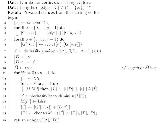
3.1.3. Dijkstra’s Algorithm for Dense Graphs

Dijkstra’s algorithm relaxes each edge only once, in the order of the distance of its start vertex from the source vertex. The edges with the same starting vertex can be relaxed in parallel. The algorithm cannot handle edges with negative weights. As Dijkstra’s algorithm only handles a few edges in parallel, Laud’s parallel reading and writing subroutines will be of little use here. Instead, we opt to use the dense representation of the graph, giving the weights of the edges in the adjacency matrix (weight “” is used to denote the lack of an edge). Our privacy-preserving implementation of Dijkstra’s algorithm is presented in Algorithm 5.
The main body of the algorithm is its last loop. It starts by finding the unhandled vertex that is closest to the source vertex. The mask vector M indicates which vertices are still unhandled. The index of this vertex is found by the function minLs given in Algorithm 6, which, when applied to a list of pairs, returns the pair with the minimal first component. We call minLs with a list where the first components are current distances, and the second components are the indices of vertices. In non-privacy-preserving implementations, priority queues can be used to find the next vertex for relaxing its outgoing edges quickly. In privacy-preserving implementations, the queues are challenging to implement efficiently due to their complex control flow. Hence, the next vertex is found by computing the minimum over the current distances for all vertices not yet handled.
Algorithm 5: Dijkstra’s algorithm
Cryptography 05 00027 i005
Algorithm 6: minLs: computing the pair with the minimal first component
Cryptography 05 00027 i006
Algorithm 5 declassifies the index of the unhandled vertex closest to the source vertex. This declassification greatly simplifies the computation of E , where the current distance of u is added to the length of all edges starting at u . Without declassification, one would need to use techniques for private reading here, which would be expensive. Note that both the computations of E and D take place in a SIMD manner, applying the same operations to E [ i ] , G [ u , i ] , D [ i ] , and M [ i ] for each i { 0 , , n 1 } .
This declassification constitutes a leak. Effectively, the last loop declassifies in which order the vertices are handled, i.e., how are the vertices ordered concerning their distance from the source vertex. Such leakage can be neutralized by randomly permuting the vertices of the graph before that last loop [9]. In this way, the indices of the vertices, when they are declassified, are random. The declassification would output a random permutation of the set { 0 , , n 1 } , one element at each iteration.
The computation of this random permutation takes place at the beginning of Algorithm 5. We first generate a private random permutation σ for n elements. We will then apply it to each row of G ; the application takes place in parallel for all rows. Similarly, we apply it to each column. Such permutation also changes the index of the source vertex, and we have to find it. We find it by taking the identity vector of length n, applying to it the inverse of σ , and then reading the position s of the resulting vector. Note that we declassify only the position s at this time, not the entire vector. At the end of the computation, we have to apply the inverse of σ to the computed vector of distances.
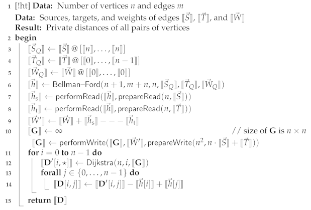
Dijkstra’s algorithm is used as a subroutine in certain APSD algorithms (Section 3.2.1). Hence, we have also implemented a vectorized version of Algorithm 5 that can compute the SSSD for several n-vertex graphs simultaneously. Below, we call this version of the algorithm nDijkstra . Obviously, Dijkstra and nDijkstra have the same round complexity. In contrast, the bandwidth usage of the latter is n times of the former (when finding SSSD for n graphs at the same time). In our empirical evaluation, we have benchmarked both versions of the algorithm.

3.1.4. Complexity of Algorithms

Two kinds of communication-related complexities matter for secure multiparty computation applications in the sense that these may become bottlenecks in deployments. First, we are interested in the bandwidth required by the algorithm, i.e., the number of bits exchanged by the computation parties. Second, we are interested in the round complexity of the algorithm, i.e., the number of round-trips that have to be made in the protocol implementing that algorithm.
Let n denote the number of vertices and m the number of edges of the graph. We assume that m is between n and O ( n 2 ) , meaning that n + m is O ( m ) and log m is O ( log n ) . We also consider the size of a single integer (used as the length of an edge or a path or as an index) to be a constant. In this case, the steps of the Bellman–Ford algorithm (Algorithm 1) before the main loop require O ( m log n ) bandwidth and O ( log n ) rounds. Indeed, both prepareRead -statements have this complexity, while the complexity of GenIndicesVector is dominated by the sorting of n private values.
Each iteration of the main loop of Algorithm 1 requires O ( m ) bandwidth and O ( log n ) rounds, with prefixMin 2 (Version 1) being the only operation working in non-constant rounds. The number of iterations is ( n 1 ) ; hence, the total bandwidth use is O ( m n ) , in O ( n log n ) rounds. However, the number of iterations reflects the worst case, which has to be taken only if no further information is available. If we know that the SSSD algorithm will be called in a context, where the shortest path(s) we’re interested in consist of at most k < n edges, then the iterating can be cut short, such that the algorithm only uses O ( m ( k + log n ) ) bandwidth in O ( k log n ) rounds.
One iteration of the main loop of Dijkstra’s algorithm (Algorithm 5) requires O ( n ) bandwidth and O ( log n ) rounds, with minLs being the only operation working in non-constant rounds. The entire loop thus requires O ( n 2 ) bandwidth and O ( n log n ) rounds. The shuffling of rows and columns before that loop also requires O ( n 2 ) bandwidth, but only constant rounds.
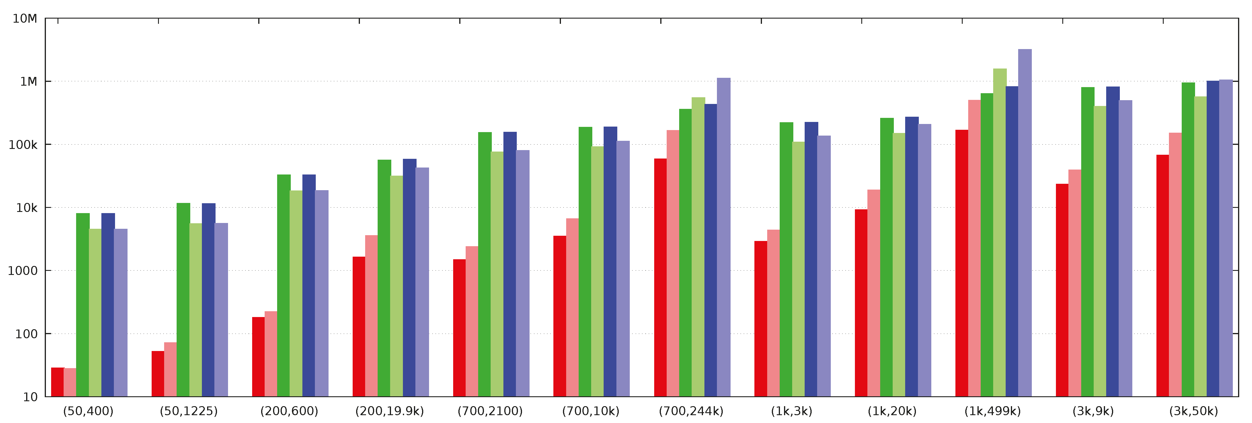
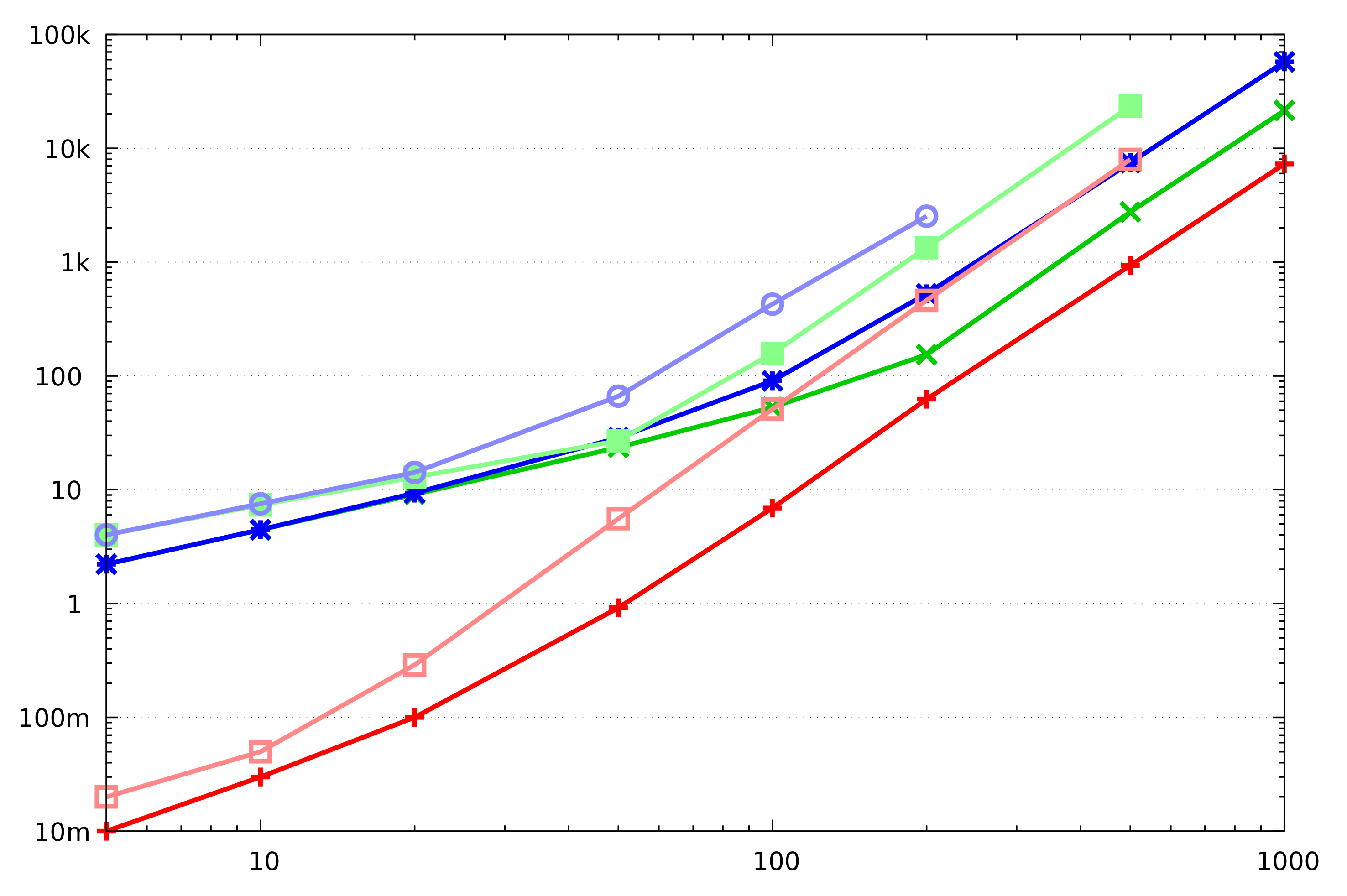
We see that Dijkstra’s algorithm requires less bandwidth than Bellman–Ford’s. Indeed, our benchmarking results (Section 3.6) confirm that. The Bellman–Ford algorithm should still be considered attractive if we can limit the number of iterations it makes. Such limitations may stem from the side information that we may have about the graph, implying that shortest paths do not have many edges. A limited number of iterations is also possible if, at the end of each iteration, we compare the current vector of distances D with its value at the previous iteration, and stop if it has not changed. This leaks the maximum number of edges on the shortest path from the given vertex; perhaps this leak can be tolerated in some scenarios. The running time of Dijkstra’s algorithm cannot be limited in such a manner.

3.1.5. Security of Algorithms

As we explained in Section 2.2, an algorithm built on top of a universally composable ABB is trivially privacy-preserving (and inherits the same security against various kinds of adversaries from the underlying secure computation protocol set) if it does not contain any declassification statements. If there are any declassifications, then we have to explain how the declassified values can be simulated based on public information only; this simulation must match the distribution of the declassified values together with private inputs. Our implementations of both SSSD algorithms have declassifications. For both of them, we have shown that the declassified values are computed by masking some private values with some randomness generated during the protocol. The result no longer depends on private values. Hence our implementations are privacy-preserving.

3.2. All-Pairs Shortest Path Algorithms

3.2.1. Johnson Algorithm

Johnson’s APSD algorithm applies Dijkstra’s algorithm at each vertex. To deal with the negative-weight edges, it will first change the weights in a manner that does not change the shortest paths. For this purpose, an extra vertex is added to the graph, with 0-weight edges from it to all existing vertices, and shortest distances h ( v ) from the new vertex to all existing vertices v are found. The weight of an edge w ( u , v ) is then updated to w ˜ ( u , v ) = w ( u , v ) + h ( u ) h ( v ) , causing the lengths of all paths from u to v to change by h ( u ) h ( v ) . Thus the shortest distances found in the modified graph, together with h, give us the shortest distances in the original graph. The shortest distances from the extra vertex are found with the Bellman–Ford algorithm.
Having the privacy-preserving implementations of both Bellman–Ford and Dijkstra algorithms, we have combined them as in Johnson’s algorithm. As our Bellman–Ford implementation expects the graph to be represented sparsely, our implementation of Johnson’s algorithm does the same. Our implementation of Dijkstra’s algorithm expects the graph to be represented in a dense manner; hence, we have to perform the conversion in the middle. Our privacy-preserving implementation of Johnson’s algorithm is given in Algorithm 7.
Algorithm 7: Johnson’s Algorithm
Cryptography 05 00027 i007
The steps of Algorithm 7 closely follow the description above. We see that we augment the original representation of the graph with an extra vertex and edges; the index of the added vertex being n, as an example S Q S @ [ n , , n ] , where @ represent the augment operation. After finding the shortest paths from this vertex to all other vertices, we use the parallel reading subroutines to find the updates for edge lengths. We then use the parallel writing subroutines to convert from sparse to a dense representation of the graph. We store the all-pairs shortest distances in the modified graph inside the matrix D , and then remove the updates to the lengths of edges (and paths).
We see that the last loop in Algorithm 7 can be performed in parallel, as there are no data dependencies between the iterations. At this point, we can use the nDijkstra procedure, discussed in Section 3.1.3. We use this procedure to fill in the entire matrix D at once and then compute D in a SIMD manner. We call the algorithm in Algorithm 7 the “Version 1” of the implementation of Johnson’s algorithm, while the version using the nDijkstra procedure is called “Version 2”. We present benchmark results for both versions.

3.2.2. Floyd–Warshall Algorithm

We implemented the Floyd–Warshall algorithm on top of the Sharemind-based ABB to compare our implementations with the previous approaches. Our implementation is standard [1,54], attempting to parallelize as many operations as possible. It uses the dense representation of the graph.
Our implementation of the SIMD-Floyd–Warshall algorithm is presented in Algorithm 8. The input data of the Floyd–Warshall algorithm is a private matrix G , which contains the weights of the edges. The output of the algorithm is a private matrix D , which has the lengths of shortest paths among all vertices in V. The algorithm has three nested loops, but the two inner ones are only used to rearrange the already computed private values and can be executed in parallel. The actual computations (addition and minimum) are made in a SIMD manner for all entries of T resp. D .
Algorithm 8: Floyd–Warshall algorithm
Cryptography 05 00027 i008

3.2.3. Transitive Closure Algorithm

In the given directed graph, checking if there is a path from vertex i to j for all vertex pairs ( i , j ) , that means vertex j is reachable. The reachability matrix is called the transitive closure of a given directed graph. We have implemented the transitive closure on top of Sharemind-based ABB to compare it with our new approach in Johnson’s APSD algorithms and with the Floyd–Warshall algorithm because the computation of transitive closure presents yet another trade-off in communication and round complexity. Our implementation of privacy-preserving APSD through transitive closure is presented in Algorithm 9. The only sequentially-run loop of the computation has a logarithmic number of iterations, so this algorithm has low round complexity in comparison with the Floyd–Warshall algorithm.

3.2.4. Complexity of Algorithms

Let us again consider the asymptotic bandwidth consumption and round complexity of our implementations. The bandwidth consumption of Johnson’s algorithm is dominated by n instances of Dijkstra’s algorithm, hence being O ( n 3 ) in total. Trivially, this is also the asymptotic bandwidth consumption of the Floyd–Warshall algorithm, but, as we see in Section 3.7, the constant hidden in the O-notation is smaller. However, Johnson’s algorithm is more versatile: if we are not interested in all-pairs shortest distances, but only in shortest distances from k < n vertices, then the bandwidth consumption of Johnson’s algorithm is only O ( m n + n 2 ( k + log n ) ) , with O ( m n ) being the bandwidth use of the Bellman–Ford algorithm and O ( n 2 log n ) the bandwidth use of the private writing into an array of size n 2 . The bandwidth consumption of the transitive closure is O ( n 3 log n ) .
Algorithm 9: Transitive closure algorithm
Cryptography 05 00027 i009
The round complexity of Johnson’s algorithm is O ( n log n ) , this being the complexity of both the Bellman–Ford and Dijkstra’s algorithms. The private reading and writing operations between them only require O ( log n ) rounds. Trivially, the round complexity of the Floyd–Warshall algorithm is O ( n ) . The round complexity of transitive closure is O ( log 2 n ) because the outer loop makes log n iterations. At each iteration, the minimal elements of vectors of length n can be found in O ( log n ) rounds.

3.2.5. Security of Algorithms

Following the discussion in Section 2.2 and Section 3.1.5, we conclude that Algorithms 7–9 are all privacy-preserving, as none of them contain any declassification statements.

3.3. Benchmarking Results in Previous Work

Extensive benchmarking results for privacy-preserving shortest path algorithms have not been reported so far. Aly et al. [8] benchmarked their implementations of Dijkstra’s and Bellman–Ford algorithms (implemented on top of VIFF [55] with BGW protocol [56] used for multiplication and Toft’s protocol [57] for comparison) on dense representations of small graphs. For Dijkstra’s algorithm on 128 vertices, they report a runtime of somewhat over an hour, while for the Bellman–Ford algorithm on 64 vertices, their running time is over 8 h. Aly and Cleemput [9] benchmark their implementation of Dijkstra’s algorithm on graphs of up to 64 vertices, reporting running times in a range of 20 s. Keller and Scholl [11] have implemented the operations of oblivious RAM (ORAM) on top of the SPDZ protocol set [34] and used them to implement a privacy-preserving version of Dijkstra’s algorithm. For cycle graphs of ca. 2000 vertices, where the graph is represented sparsely, they report the running times in a couple of minutes. For general graphs, represented densely, their implementation requires a couple of hours for graphs with 500 vertices. Carter et al. [58] use garbled circuits (hence removing considerations about round complexity but consuming more bandwidth) to evaluate Dijkstra’s algorithm privately. They report running times of ca. 15 min for 100-vertex graphs (their parallel implementation handles 32 circuits simultaneously on a 32-core server). Similarly, Liu et al. [59] make use of garbled circuits to evaluate Dijkstra’s algorithm on sparse graphs, employing oblivious priority queues [60] to increase efficiency. The estimate is that together with JustGarble [61], their running time on a 1000-vertex, 3000-edge graph is maybe 20 min. No evaluation is reported in [62].

3.4. Setup for Our Experiments

We implemented all algorithms described above on top of Sharemind’s three-party protocol set secure against one passively corrupted party [16,17], making use of the SecreC high-level language [33] and other development tools included with the Sharemind platform. We have used 32-bit integers for all weights and indices. We benchmarked our implementations on a cluster of three servers with 12-core 3 GHz CPUs with Hyper-Threading running Linux and 48 GB of RAM, connected by an Ethernet local area network with a link speed of 1 Gbps. However, note that Sharemind’s implementation is single-threaded; hence, we have not taken advantage of multiple cores performing local operations, nor the possibility of doing computations and communications simultaneously.
As our protocols cover a vast space of trade-offs between bandwidth consumption and round complexity, their relative performance over different networks may be different. For characterizing the variation in performance, we have benchmarked our protocols in three different environments, throttling the connection between the servers in our cluster. In the “high-bandwidth” setting, the link speeds between servers are 1 Gbps, while in the “low-bandwidth” setting, the speeds are 100 Mbps. In the “low-latency” setting, we have not delayed the messages between the servers, while in the “high-latency” setting, the messages are delayed by 40ms. We have run our experiments in “high-bandwidth low-latency” (HBLL) environment (i.e., in our local area network), as well as in “high-bandwidth high-latency” (HBHL) and “low-bandwidth high-latency” (LBHL) environments, simulating wide-area networks with different characteristics.

3.5. Bellman–Ford Algorithm Experiments

3.5.1. Bellman–Ford Algorithm in the HBLL Environment

The execution time of our privacy-preserving Bellman–Ford algorithm depends only on its public inputs, i.e., the number of vertices n and the number of edges m of the graph. We report the running times in Table 1 for various sizes of the input graph. Suffixes “k” and “M” mean multiplication by 1000 and 1,000,000, respectively. “Version 1” of the algorithm uses the implementation of prefixMin 2 shown in Algorithm 3, while “Version 2” uses the implementation shown in Algorithm 4. The executions of the algorithm are made in the “high-bandwidth low-latency” environment.
The execution of the Bellman–Ford algorithm consists of preparatory steps for subsequent array accesses according to private indices, followed by the main loop of the algorithm executed at most ( n 1 ) times. In Table 1, we report separately the time it took to run the preparatory steps of Algorithm 1 (everything up to the main loop), as well as the main loop (all ( n 1 ) iterations).
As part of some larger applications, we may want to execute the Bellman–Ford algorithm for less than ( n 1 ) iterations. Perhaps we know from the context that a smaller number of iterations is sufficient, or perhaps it is acceptable to leak either the precise number of iterations or some padded version of it. Given the number of vertices and edges, as well as the expected number of iterations, Table 1 can be used to find the expected running time. Indeed, one has to take the running time of the preprocessing and add to it a fraction of the running time for the main loop, where the fraction is equal to the proportion of the number of iterations to the number of vertices.
In benchmarking, we attempted to consider both dense and sparse graphs. An interesting class among sparse graphs are planar graphs, which are expected to show up in various applications. Hence, ca. half of our tests were run with graphs whose number of edges matches that of typical planar graphs having mostly triangles as faces—we let the number of edges be thrice its number of vertices.

3.5.2. Effect of Network Bandwidth and Latency to Bellman–Ford Algorithm

Version 1 of our implementation of the Bellman–Ford algorithm consumes less bandwidth, while Version 2 has better round complexity. This difference can be seen in Table 1, where either implementation may have a smaller running time for certain sizes of inputs.
We benchmarked both versions of the Bellman–Ford algorithm in different network environments for graphs of various sizes. We give both the running time and bandwidth consumption in Appendix A. We also depict the running time in Figure 1.
The timing results clearly show that the two different versions of the algorithm behave very differently in different network environments. While Version 1 of the algorithm is always better in the HBLL environment, it depends on the number of edges of the graph for the environments with high latency. Indeed, the number of edges essentially determines the parallelism available for the algorithm; a small number of edges makes Version 2 preferable because of its smaller round complexity.
The timing results also show that for all sizes of the graph shown in Figure 1, the performance of the algorithm is essentially bounded by the latency of the network. Indeed, for smaller examples, we see very little difference between the HBHL and LBHL environments. Moreover, even for the largest examples, there is still a very significant difference between the HBLL and HBHL environments.

3.6. Dijkstra’s Algorithm Experiments

3.6.1. Dijkstra’s Algorithm in the HBLL Environment

The running time of our privacy-preserving Dijkstra’s algorithm depends only on the number n of the vertices of the input graph. We report the running times in Table 2 for various values of n. For interest and similarly to [9], for some of the instances, we report separately the time it takes to permute the vertices and the time it takes to execute the main loop of Algorithm 5. For most use cases, this split is only informative because all iterations of the main loop have to be executed to find the shortest distances to all vertices. It may be useful only if we are interested in the shortest path from the source vertex s to some target vertex t, and we somehow know that t is one of the closest vertices to s. Again, the running times are given for the HBLL environment.
Comparing Table 1 and Table 2, we see that generally, Dijkstra’s algorithm performs faster than the Bellman–Ford algorithm. This is expected because the main loop of both algorithms makes n iterations. Still, the amount of work done in one iteration of the Bellman–Ford algorithm is O ( m ) , while the amount of work done in one iteration of Dijkstra’s algorithm is O ( n ) . On the other hand, the Bellman–Ford algorithm works on the sparse representation of the graph, while Dijkstra’s algorithm requires the dense representation. Hence the memory consumption of the latter may be significantly higher for sparse graphs. Dijkstra’s algorithm can be made to work on sparse representation of the graph, using oblivious RAM and loop coalescing [59]. However, this will increase the number of iterations to O ( m ) , which is undesirable when the actual performance of the algorithm is latency-bound.
In Figure 2 and Figure 3, we present a graphical comparison of the performance of Dijkstra’s and Bellman–Ford algorithms (in HBLL environment) on certain small and medium-size graphs. We have evaluated the performance for certain pairs ( n , m ) of the number of vertices and edges for sparse graphs. For dense graphs, the horizontal axis shows the number of vertices n, while the number of edges is n ( n 1 ) / 2 . For graphs where the number of edges is similar to planar graphs, we chose their numbers to be two or three times the number of vertices. We see that Dijkstra’s algorithm is more efficient in all cases, but the difference is less pronounced for sparse graphs.

3.6.2. Effect of Network Bandwidth and Latency to Dijkstra’s Algorithm

In different network environments, we expect Dijkstra’s algorithm to behave similarly to the Bellman–Ford algorithm—it will also be latency-bound to an even greater extent. Considering our privacy-preserving implementations of Johnson’s algorithm, a more interesting question is about the behavior of Dijkstra’s algorithm when it is executed several times over graphs of the same size. While the sequential execution will be latency-bound similarly to a single execution, the parallel execution may use the available bandwidth more fully.
In Figure 4, we establish the baseline for our experiments, measuring the running time of Dijkstra’s algorithm on graphs of different sizes in different network environments. These are the running times for finding the SSSD in a single graph. We see that the performance is very much latency-bound, such that the available bandwidth even does not affect the performance on most graphs in high-latency environments.
We would like to characterize the performance gains resulting from the parallel execution on multiple graphs in a meaningful manner that is comparable over a different number of graphs, graph sizes, and network environments. If t 1 is the time it takes to execute the algorithm on one graph, for a given size of the graph and the network environment, and t k is the time it takes to execute the algorithm on k graphs, then we would like to state that the gains are maximal, if t k t 1 , and minimal, if t k k · t 1 . We would then map the gains to the segment [ 0 , 1 ] .
Serial fraction [63] is such a measure. In our terms, it is expressed as f k = ( t k / t 1 1 ) / ( k 1 ) . It characterizes how much of the computation has not benefited from the parallelization. In Figure 5, we present the measurement of the serial fraction when running multiple copies of Dijkstra’s algorithm in parallel, for different sizes of graphs, different numbers of copies, and different network environments. We have not tested the parallel execution for a number of graphs larger than the number of vertices in a graph because this case will not be needed in any sensible executions of Johnson’s algorithm. We see that the largest gains are for the HBHL environment, as expected. Interestingly, at least for high-latency environments, the largest gains are obtained for graphs with ca. 200 vertices. This may mean that the parallelization possibilities for computations with a single graph for larger graphs are already significant.
In Appendix A, we present the data underlying Figure 4 and Figure 5: the running times obtained by benchmarking Dijkstra’s algorithm with various inputs and in various network environments.

3.7. All Pairs Shortest Paths EXPERIMENTS

3.7.1. APSD Algorithms in the HBLL Environment

The execution time of our privacy-preserving Floyd–Warshall algorithm and transitive closure computation also depends only on the number n of the vertices of the input graph. We report the running times in Table 3 for various values of n.
As our implementation of Johnson’s algorithm starts from the sparse representation, its running time depends both on the number n of vertices and the number m of edges of the input graph. We report the running times for certain dense graphs in Table 3. The algorithm consists of three clearly identifiable stages—execution of the Bellman–Ford algorithm, updating of the lengths of edges, and execution of n copies of Dijkstra’s algorithm. We report the running time of each stage for two versions of Johnson’s algorithm. Recall that in Version 1, n copies of Dijkstra’s algorithm are executed one after another. In Version 2, they are all executed in parallel. The benchmarking is done in the HBLL environment. We see that the parallelization gains are smaller for small graphs due to the first, non-parallelizable steps taking relatively more time. We also see the parallelization gains drop for larger graphs, similarly to the benchmarking outcomes shown in Figure 5 (HBLL plots, right edge of the figure).
Table 3 shows that transitive closure is not competitive with Floyd–Warshall, even though its round complexity is smaller. It also shows Johnson’s algorithm requiring significantly more time than Floyd–Warshall. However, the latter is not a good comparison, as Table 3 only presents the worst-case running time for Johnson’s algorithm for graphs with a given number of vertices. Indeed, the following aspects may improve the running time:
  • If the number of edges is smaller, then the execution of the Bellman–Ford step needs less time.
  • The execution time of the Bellman–Ford step may be smaller if it is run for a smaller number of iterations (see discussion in Section 3.5).
  • If the shortest distances have to be found only from a subset of vertices, then a smaller number of instances of Dijkstra’s algorithm has to be executed.
None of these aspects applies to the Floyd–Warshall algorithm. The consequences on running time from all of these aspects have been covered in our benchmarks, in Table 1 and Figure 5.

3.7.2. Bandwidth vs. Latency of Privacy-Preserving APSD Algorithms

In Figure 6, we present the comparison of Floyd–Warshall and transitive closure algorithms for different network environments. We see that despite the lower round complexity, transitive closure is still slower also in high-latency environments. The running times that we measured are given in Appendix A.
We did not include Johnson’s algorithm in this comparison due to the significant number of tunable parameters. The benchmarking results we reported previously allow one to estimate the performance of different stages of Johnson’s algorithm for various values of these parameters and in different networking environments.

4. Discussion

We demonstrated how to use state-of-the-art algorithmic techniques of private computation to implement privacy-preserving versions of classical SSSD and APSD algorithms. We implemented and benchmarked these algorithms, giving a good idea of how efficient they are on top of secure multiparty computation protocols in different deployments. Significant details in our privacy-preserving algorithms are novel, particularly in the adaptation of the Bellman–Ford algorithm to privacy-preserving computations and in the connection. Such compilation and evaluation of privacy-preserving shortest paths have not been done before. In particular, our evaluation of APSD algorithms is not similar to any previous work.
We see that the performance of privacy-preserving SSSD and APSD algorithms depends on the size of the input graph. Still, it may be improved by using some side information publicly available about that graph or about the actual privacy-preserving task at hand. For example, we see that generally, Dijkstra’s algorithm for dense graphs is more efficient than Bellman–Ford for sparse graphs, even if the number of edges is low, the running time of the latter may be significantly decreased if it is known that the shortest paths only have a number of edges that is much smaller than the total number of vertices in the graph. Similar considerations apply for APSD and the choice between Floyd–Warshall and Johnson algorithms. Our benchmarking results can be used to deduce the likely running times of our algorithms as subroutines for a wide variety of applications in different network settings. The running times we achieve are orders of magnitude smaller than those reported in previous work in certain settings.
The future work on privacy-preserving shortest path algorithms may encompass the search for some more parallelization opportunities. However, the underlying algorithms may perhaps not be amenable to many more possibilities. The use of oblivious data structures may bring down the bandwidth requirements of Dijkstra’s algorithm applied to sparse graphs, but probably not its round complexity.

Author Contributions

Conceptualization: M.A. and P.L.; methodology: M.A. and P.L.; software: M.A.; investigation: M.A.; visualization: M.A. and P.L.; writing—original draft: M.A. and P.L.; supervision: P.L. and E.V.; project management: P.L.; funding acquisition: P.L. and E.V. All authors have read and agreed to the published version of the manuscript.

Funding

This research received funding from the European Regional Development Fund through the Estonian Centre of Excellence in ICT Research—EXCITE.

Institutional Review Board Statement

Not applicable.

Informed Consent Statement

Not applicable.

Data Availability Statement

The benchmarking results discussed in this article are available in the Appendix A.

Conflicts of Interest

The authors declare no conflict of interest.

Appendix A. Execution Time and Bandwidth Consumption for Privacy-Preserving Shortest Distance Algorithms in Different Network Environments

Table A1. Benchmarking results (bandwidth for a single computing server) for Bellman–Ford algorithms in different network environments.
Size ofVersion 1 (with Algorithm 3)Version 2 (with Algorithm 4)
GraphBand-Running Time (s)Band-Running Time (s)
nmWidthHBLLHBHLLBHLWidthHBLLHBHLLBHL
5040032 MB2.8799799.565 MB2.8448451
50122574 MB5.211551145206 MB7.2550559
200600165 MB17.932703261465 MB22.218231841
20019.9 k2900 MB1625626580615.8 GB356.231224219
70021001570 MB14715.4 k15.4 k6.3 GB237.775297956
70010 k5 GB34818.5 k18.7 k27 GB661.7915811.1 k
700244 k110 GB582335.9 k42.9 k810 GB16.4 k54.2 k111 k
1 k3 k4 GB28822 k22.2 k12.7 GB435.810.8 k13.5 k
1 k20 k13 GB91725.9 k26.7 k90 GB187914.8 k20.6 k
1 k499 k320 GB16.6 k63.4 k81.7 k2.4 TB49.8 k156 k318 k
3 k9 k65 GB231879.6 k81.1 k145 GB388939.8 k49.3 k
3 k50 k133 GB667593.3 k100 k630 GB15 k56.3 k104 k
Table A2. Benchmarking results for the parallel execution of Dijkstra’s algorithm on several graphs of the same size, in different network environments.
Num. ofSize ofRunning Time (s)
GraphsGraphHBLLHBHLLBHL
1100.0921.629.3
10100.254.154.1
1250.2373.4100.7
25251.0158.4160.6
1500.53166.8228.9
5501.6326.0326.8
10502.6329.8331.8
25503.9336.9341.9
50506.3371.1388.4
11001.29373.8513.7
101007.5745.4755.2
2510016.1764.2792.2
5010028.6793.5852.3
7510042.6834.7920.8
10010042.3898.11019
12003.37828.31144
2020046.016991792
50200104.818002075
100200189.321382787
200200337.626573669
150012.528844042
1005001049752410.8 k
500500371517.2 k34.6 k
1100046.163568933
501000212915.7 k21.0 k
500100021.1 k62.2 k125 k
1000100042.5 k109 k235 k
15000853.440.8 k61.2 k
1005000230 k390 k648.9 k
Table A3. Benchmarking results (bandwidth for a single computing server) for Floyd–Warshall and transitive closure algorithms in different network environments.
SizeFloyd–WarshallTransitive Closure
ofBand-Running Time (s)Band-Running Time (s)
GraphWidthHBLLHBHLLBHLWidthHBLLHBHLLBHL
50.08 MB0.012.222.220.46 MB0.024.014.01
100.48 MB0.034.444.461.64 MB0.057.377.53
203.52 MB0.19.19.3516.4 MB0.2912.914.2
5054.1 MB0.9223.628.6318 MB5.5626.966.3
100402.2 MB6.9152.990.53019 MB51.1157.7426.6
2003417 MB62.4153.652627.3 GB460.513362529
50053.3 GB93427537469490 GB798723.5 k
1 k426 GB726821.5 k57.4 k

References

  1. Brickell, J.; Shmatikov, V. Privacy-preserving graph algorithms in the semi-honest model. In International Conference on the Theory and Application of Cryptology and Information Security; Springer: Berlin/Heidelberg, Germany, 2005; pp. 236–252. [Google Scholar]
  2. Yao, A.C. Protocols for Secure Computations (Extended Abstract). In Proceedings of the 23rd Annual Symposium on Foundations of Computer Science, Chicago, IL, USA, 3–5 November 1982; pp. 160–164. [Google Scholar] [CrossRef]
  3. Chaum, D.; Crépeau, C.; Damgård, I. Multiparty Unconditionally Secure Protocols (Extended Abstract). In Symposium on Theory of Computing (STOC); ACM: New York, NY, USA, 1988; pp. 11–19. [Google Scholar]
  4. Goldreich, O.; Micali, S.; Wigderson, A. How to Play any Mental Game or A Completeness Theorem for Protocols with Honest Majority. In Symposium on Theory of Computing (STOC); ACM: New York, NY, USA, 1987; pp. 218–229. [Google Scholar]
  5. Pippenger, N.; Fischer, M.J. Relations among complexity measures. J. ACM 1979, 26, 361–381. [Google Scholar] [CrossRef] [Green Version]
  6. Shamir, A. How to Share a Secret. Commun. ACM 1979, 22, 612–613. [Google Scholar] [CrossRef]
  7. Cormen, T.H.; Leiserson, C.E.; Rivest, R.L.; Stein, C. Introduction to Algorithms; MIT Press: Cambridge, MA, USA, 2009. [Google Scholar]
  8. Aly, A.; Cuvelier, E.; Mawet, S.; Pereira, O.; Van Vyve, M. Securely Solving Simple Combinatorial Graph Problems. In Financial Cryptography; Springer: Berlin/Heidelberg, Germany, 2013; pp. 239–257. [Google Scholar]
  9. Aly, A.; Cleemput, S. An Improved Protocol for Securely Solving the Shortest Path Problem and its Application to Combinatorial Auctions. Cryptol. EPrint Arch. Rep. 2017, 2017, 971. [Google Scholar]
  10. Goldreich, O.; Ostrovsky, R. Software Protection and Simulation on Oblivious RAMs. J. ACM 1996, 43, 431–473. [Google Scholar] [CrossRef] [Green Version]
  11. Keller, M.; Scholl, P. Efficient, oblivious data structures for MPC. In International Conference on the Theory and Application of Cryptology and Information Security; Springer: Berlin/Heidelberg, Germany, 2014; pp. 506–525. [Google Scholar]
  12. Liu, C.; Huang, Y.; Shi, E.; Katz, J.; Hicks, M. Automating Efficient RAM-Model Secure Computation. In Proceedings of 2014 IEEE Symposium on Security and Privacy, Berkeley, CA, USA, 18–21 May 2014; pp. 623–638. [Google Scholar]
  13. Bellman, R. On a routing problem. Q. Appl. Math. 1985, 16, 87–90. [Google Scholar] [CrossRef] [Green Version]
  14. Laud, P. Parallel oblivious array access for secure multiparty computation and privacy-preserving minimum spanning trees. Proc. Priv. Enhancing Technol. 2015, 2015, 188–205. [Google Scholar] [CrossRef] [Green Version]
  15. Dijkstra, E.W. A note on two problems in connexion with graphs. Numer. Math. 1959, 1, 269–271. [Google Scholar] [CrossRef] [Green Version]
  16. Bogdanov, D.; Niitsoo, M.; Toft, T.; Willemson, J. High-performance secure multi-party computation for data mining applications. Int. J. Inf. Secur. 2012, 11, 403–418. [Google Scholar] [CrossRef]
  17. Bogdanov, D.; Laur, S.; Willemson, J. Sharemind: A framework for fast privacy-preserving computations. In European Symposium on Research in Computer Security (ESORICS); Springer: Berlin/Heidelberg, Germany, 2008; pp. 192–206. [Google Scholar]
  18. Damgård, I.; Nielsen, J.B. Universally Composable Efficient Multiparty Computation from Threshold Homomorphic Encryption. In Proceedings of the Advances in Cryptology—CRYPTO 2003, 23rd Annual International Cryptology Conference, Santa Barbara, CA, USA, 17–21 August 2003; Proceedings (Lecture Notes in Computer Science, Vol. 2729). Boneh, D., Ed.; Springer: Berlin/Heidelberg, Germany, 2003; pp. 247–264. [Google Scholar]
  19. Gennaro, R.; Rabin, M.O.; Rabin, T. Simplified VSS and Fast-Track Multiparty Computations with Applications to Threshold Cryptography. In Proceedings of the Seventeenth Annual ACM Symposium on Principles of Distributed Computing, PODC ’98, Puerto Vallarta, Mexico, 28 June–2 July 1998; Yehuda Afek, B.A.C., Ed.; ACM: New York, NY, USA, 1998; pp. 101–111. [Google Scholar]
  20. Agrawal, R.; Srikant, R. Privacy-preserving data mining. In Proceedings of the 2000 ACM SIGMOD International Conference on Management of Data, Dallas, TX, USA, 15–18 May 2000; pp. 439–450. [Google Scholar]
  21. Lindell, Y.; Pinkas, B. Privacy Preserving Data Mining. J. Cryptol. 2000, 15, 177–206. [Google Scholar] [CrossRef]
  22. Mendes, R.; Vilela, J.P. Privacy-preserving data mining: Methods, metrics, and applications. IEEE Access 2017, 5, 10562–10582. [Google Scholar] [CrossRef]
  23. Ostrak, A.; Randmets, J.; Sokk, V.; Laur, S.; Kamm, L. Implementing Privacy-Preserving Genotype Analysis with Consideration for Population Stratification. Cryptography 2021, 5, 21. [Google Scholar] [CrossRef]
  24. Freedman, M.J.; Nissim, K.; Pinkas, B. Efficient private matching and set intersection. In International Conference on the Theory and Applications of Cryptographic Techniques; Springer: Berlin/Heidelberg, Germany, 2004; pp. 1–19. [Google Scholar]
  25. Saldamli, G.; Ertaul, L.; Dholakia, K.; Sanikommu, U. An Efficient Private Matching and Set Intersection Protocol: Implementation PM-Malicious Server. In Proceedings of the International Conference on Security and Management (SAM), The Steering Committee of the World Congress in Computer Science, Las Vegas, NV, USA, 29 July–1 August 2019; pp. 16–22. [Google Scholar]
  26. Naor, M.; Pinkas, P.; Sumner, R. Privacy preserving auctions and mechanism design. In Proceedings of the 1st ACM Conference on Electronic Commerce, Denver, CO, USA, 3–5 November 1999; pp. 129–139. [Google Scholar]
  27. Kissner, L.; Song, D. Privacy-preserving set operations. In Annual International Cryptology Conference; Springer: Berlin/Heidelberg, Germany, 2005; pp. 241–257. [Google Scholar]
  28. Anagreh, M.; Vainikko, E.; Laud, P. Parallel Privacy-preserving Computation of Minimum Spanning Trees. In Proceedings of the 7th International Conference on Information Systems Security and Privacy—ICISSP, online, 11–13 February 2021; pp. 181–190, ISBN 978-989-758-491-6. ISSN 2184-4356. [Google Scholar] [CrossRef]
  29. Laud, P.; Pankova, A.; Kamm, L.; Veeningen, M. Basic Constructions of Secure Multiparty Computation. In Applications of Secure Multiparty Computation; Laud, P., Kamm, L., Eds.; IOS Press: Amsterdam, The Netherlands, 2015; pp. 1–25. [Google Scholar]
  30. Laud, P. Stateful abstractions of secure multiparty computation. In Applications of Secure Multiparty Computation; Laud, P., Kamm, L., Eds.; IOS Press: Amsterdam, The Netherlands, 2015; pp. 26–42. [Google Scholar]
  31. Canetti, R. Security and composition of multiparty cryptographic protocols. J. Cryptol. 2000, 13, 143–202. [Google Scholar] [CrossRef]
  32. Laur, S.; Pullonen-Raudvere, P. Foundations of Programmable Secure Computation. Cryptography 2021, 5, 22. [Google Scholar] [CrossRef]
  33. Bogdanov, D.; Laud, P.; Randmets, J. Domain-Polymorphic Programming of Privacy-Preserving Applications. In Proceedings of the Ninth Workshop on Programming Languages and Analysis for Security, PLAS@ECOOP2014, Uppsala, Sweden, 29 July 2014; Russo, A., Tripp, O., Eds.; ACM: New York, NY, USA, 2014; pp. 53–65. [Google Scholar]
  34. Damgård, I.; Pastro, V.; Smart, P.; Zakarias, S. Multi-party Computation from Somewhat Homomorphic Encryption. In Proceedings of the Advances in Cryptology—CRYPTO 2012—32nd Annual Cryptology Conference, Santa Barbara, CA, USA, 19–23 August 2012; Proceedings (Lecture Notes in Computer Science, Vol. 7417). Reihaneh Safavi-Naini, R., Canetti, R., Eds.; Springer: Berlin/Heidelberg, Germany, 2012; pp. 643–662. [Google Scholar]
  35. Laur, S.; Willemson, J.; Zhang, B. Round-Efficient Oblivious Database Manipulation. In Proceedings of the Information Security, 14th International Conference, ISC 2011, Xi’an, China, 26–29 October 2011; Proceedings (Lecture Notes in Computer Science, Vol. 7001). Lai, X., Zhou, J., Li, H., Eds.; Springer: Berlin/Heidelberg, Germany, 2011; pp. 262–277. [Google Scholar]
  36. Laud, P. Linear-time oblivious permutations for SPDZ. 2021; submitted. [Google Scholar]
  37. Bogdanov, D.; Laur, S.; Talviste, R. A Practical Analysis of Oblivious Sorting Algorithms for Secure Multi-party Computation. In Proceedings of the Secure IT Systems-19th Nordic Conference, NordSec 2014, Tromsø, Norway, 15–17 October 2014; Proceedings (Lecture Notes in Computer Science, Vol. 8788). Bernsmed, K., Fischer-Hübner, S., Eds.; Springer: Berlin/Heidelberg, Germany, 2014; pp. 59–74. [Google Scholar]
  38. Anagreh, M.; Vainikko, E.; Laud, P. Parallel Privacy-Preserving Shortest Paths by Radius-Stepping. In Proceedings of the 2021 29th Euromicro International Conference on Parallel, Distributed and Network-Based Processing (PDP), Valladolid, Spain, 10–12 March 2021; pp. 276–280. [Google Scholar]
  39. Blelloch, G.E.; Gu, Y.; Sun, Y.; Tangwongsan, K. Parallel shortest paths using radius stepping. In Proceedings of the 28th ACM Symposium on Parallelism in Algorithms and Architectures, Pacific Grove, CA, USA, 11–13 July 2016; ACM: New York, NY, USA, 2016; pp. 443–454. [Google Scholar]
  40. Meyer, U.; Sanders, P. Δ-stepping: A parallelizable shortest path algorithm. J. Algorithms 2003, 49, 114–152. [Google Scholar] [CrossRef] [Green Version]
  41. Wu, D.J.; Zimmerman, J.; Planul, J.; Mitchell, J.C. Privacy-Preserving Shortest Path Computation. In Proceedings of the 23rd Annual Network and Distributed System Security Symposium, NDSS 2016, San Diego, CA, USA, 21–24 February 2016; The Internet Society: Reston, VA, USA, 2016. [Google Scholar]
  42. Ramezanian, S.; Meskanen, T.; Niemi, V. Privacy Preserving Shortest Path Queries on Directed Graph. In Proceedings of the 2018 22nd Conference of Open Innovations Association (FRUCT), Jyvaskyla, Finland, 15–18 May 2018; pp. 217–223. [Google Scholar]
  43. Matsumoto, K.; Nakasato, N.; Sedukhin, S.G. Blocked united algorithm for the all-pairs shortest paths problem on hybrid CPU-GPU systems. IEICE Trans. Inf. Syst. 2012, 95, 2759–2768. [Google Scholar] [CrossRef] [Green Version]
  44. Nepomniaschaya, A.S. Concurrent selection of the shortest paths and distances in directed graphs using vertical processing systems. Bull. Novosib. Comput. Cent. 2003, 19, 61–72. [Google Scholar]
  45. Han, S.C.; Kang, S.C. Optimizing All Pairs Shortest Path Algorithm Using Vector Instructions. Project Report, Carnegie-Mellon University. 2005. Available online: https://users.ece.cmu.edu/~pueschel/teaching/18-799B-CMU-spring05/material/sungchul-sukchan.pdf (accessed on 12 October 2021).
  46. Takei, Y.; Hariyama, M.; Kameyama, M. Evaluation of an FPGA-based shortest-path-search accelerator. In Proceedings of the International Conference on Parallel and Distributed Processing Techniques and Applications (PDPTA), Las Vegas, USA, 27–30 July 2015; p. 613. [Google Scholar]
  47. Nagavalli, S. Dynamic Optimization—Using Hardware Parallelism for Faster Search via Dynamic Programming. Project Report, Carnegie-Mellon University. 2013. Available online: https://www.andrew.cmu.edu/user/snagaval/16-745/Project/16-745-Project-Report-SasankaNagavalli.pdf (accessed on 12 October 2021).
  48. Klein, P.N.; Subramanian, S. A randomized parallel algorithm for single-source shortest paths. J. Algorithms 1997, 25, 205–220. [Google Scholar] [CrossRef] [Green Version]
  49. Meyer, U. Design and Analysis of Sequential and Parallel Single-Source Shortest-Paths Algorithms. Ph.D. Dissertation, University of Saarland, Saarbrücken, Germany, 2002. [Google Scholar]
  50. Träff, J.L.; Zaroliagis, C.D. A simple parallel algorithm for the single-source shortest path problem on planar digraphs. In Proceedings of the International Workshop on Parallel Algorithms for Irregularly Structured Problems, Santa Barbara, CA, USA, 19–21 August 1996; Springer: Berlin/Heidelberg, Germany, 1996; pp. 183–194. [Google Scholar]
  51. Gentry, C.; Halevi, S.; Lu, S.; Ostrovsky, R.; Raykova, M.; Wichs, D. Garbled RAM Revisited. In Proceedings of the Advances in Cryptology—EUROCRYPT 2014—33rd Annual International Conference on the Theory and Applications of Cryptographic Techniques, Copenhagen, Denmark, 11–15 May 2014; Proceedings (Lecture Notes in Computer Science, Vol. 8441). Nguyen, P.Q., Oswald, E., Eds.; Springer: Berlin/Heidelberg, Germany, 2014; pp. 405–422. [Google Scholar]
  52. Ladner, R.E.; Fischer, M.J. Parallel prefix computation. J. ACM 1980, 27, 831–838. [Google Scholar] [CrossRef]
  53. Hillis, W.; Steele, G. Data parallel algorithms. Commun. ACM 1986, 29, 1170–1183. [Google Scholar] [CrossRef]
  54. Kerschbaum, F.; Schaad, A. Privacy-preserving social network analysis for criminal investigations. In Proceedings of the 2008 ACM Workshop on Privacy in the Electronic Society, WPES 2008, Alexandria, VA, USA, 27 October 2008; Atluri, V., Winslett, M., Eds.; ACM: New York, NY, USA, 2008; pp. 9–14. [Google Scholar]
  55. Geisler, M. Cryptographic Protocols: Theory and Implementation. Ph.D. Dissertation, Aarhus University, Aarhus, Denmark, 2010. [Google Scholar]
  56. Ben-Or, M.; Goldwasser, S.; Wigderson, A. Completeness Theorems for Non-Cryptographic Fault-Tolerant Distributed Computation (Extended Abstract). In Proceedings of the 20th Annual ACM Symposium on Theory of Computing, Chicago, IL, USA, 2–4 May 1988; Simon, J., Ed.; ACM: New York, NY, USA, 1988; pp. 1–10. [Google Scholar]
  57. Toft, T. Primitives and Applications for Multi-Party Computation. Ph.D. Dissertation, University of Aarhus, Aarhus, Denmark, 2007. [Google Scholar]
  58. Carter, H.; Mood, B.; Traynor, P.; Butler, K.R. Secure Outsourced Garbled Circuit Evaluation for Mobile Devices. In Proceedings of the 22th USENIX Security Symposium, Washington, DC, USA, 14–16 August 2013; King, S.T., Ed.; USENIX Association: Berkeley, CA, USA, 2013; pp. 289–304. [Google Scholar]
  59. Liu, C.; Wang, X.S.; Nayak, N.; Huang, Y.; Shi, E. ObliVM: A Programming Framework for Secure Computation. In Proceedings of the 2015 IEEE Symposium on Security and Privacy, SP 2015, San Jose, CA, USA, 17–21 May 2015; pp. 359–376. [Google Scholar] [CrossRef]
  60. Wangat, X.S. Oblivious Data Structures. In Proceedings of the 2014 ACM SIGSAC Conference on Computer and Communications Security, Scottsdale, AZ, USA, 3–7 November 2014; Ahn, G.J., Yung, M., Li, N., Eds.; ACM: New York, NY, USA, 2014; pp. 15–226. [Google Scholar]
  61. Bellare, M.; Hoang, V.T.; Keelveedhi, S.; Rogaway, P. Efficient Garbling from a Fixed-Key Block cipher. In Proceedings of the 2013 IEEE Symposium on Security and Privacy, SP 2013, Berkeley, CA, USA, 19–22 May 2013; pp. 478–492. [Google Scholar]
  62. Blanton, M.; Steele, A.; Aliasgari, M. Data-oblivious graph algorithms for secure computation and outsourcing. In Proceedings of the 8th ACM Symposium on Information, Computer and Communications Security, ASIA CCS ’13, Hangzhou, China, 8–10 May 2013; Chen, K., Xie, Q., Qiu, W., Li, N., Tzeng, W.G., Eds.; ACM: New York, NY, USA, 2013; pp. 207–218. [Google Scholar]
  63. Karp, A.H.; Flatt, H.P. Measuring Parallel Processor Performance. Commun. ACM 1990, 33, 539–543. [Google Scholar] [CrossRef]
Figure 1. Bellman-Ford algorithm performance (time in seconds) in different networks for different ( n , m ) (red: HBLL, green: HBHL, blue: LBHL, dark: Version 1, light: Version 2).
Cryptography 05 00027 g001
Figure 2. Performance (in seconds) comparison of Dijkstra’s (blue) and Bellman–Ford (red) algorithms on sparse and dense graphs.
Cryptography 05 00027 g002
Figure 3. Performance (in seconds) comparison of Dijkstra’s (blue) and Bellman–Ford (light red: m = 3 n ; dark red: m = 2 n ) algorithms on planar-like graphs.
Cryptography 05 00027 g003
Figure 4. Performance (in seconds) of Dijkstra’s algorithm on graphs with given numbers of vertices in different network environments (red: HBLL, green: HBHL, blue: LBHL).
Cryptography 05 00027 g004
Figure 5. Dijkstra’s algorithm performance (as serial fraction; lower is better) on multiple graphs of various sizes (number of vertices given on the graph) in different network environments (red: HBLL, green: HBHL, blue: LBHL).
Cryptography 05 00027 g005
Figure 6. Performance (time in seconds) of Floyd–Warshall and transitive closure algorithms on graphs of different sizes in different network environments (red: HBLL, green: HBHL, blue: LBHL, dark: Floyd–Warshall, light: transitive closure).
Cryptography 05 00027 g006
Table 1. Running times (in seconds) of privacy-preserving Bellman–Ford Algorithm.
Graph BF Version 2BF Version 1
nmPre.LoopTotalLoopTotal
1025 0.18 0.27
20100 0.53 0.70
50400 2.68 2.70
851200 11.3 8.10
1702500 37.8 25.8
35010509.442.752.127.536.9
35020009.468.978.341.651.0
500150018.987.3106.254.173.0
500500019.7195.0214.7121.4140.7
700210037.3165.5202.8109.5146.8
70010 k38.2476.1514.3291.1329.3
30009 k6632541320415452208
300050 k67610,51111,18754156091
450013.5 k15155830734532394754
4500100 k1.5 k 16.2 k17.7 k
700021 k3.6 k 7.7 k11.3 k
7000200 k3.6 k 46.6 k50.2 k
850025.5 k5.2 k 11.2 k16.4 k
8500300 k5.3 k 81.7 k87 k
950028.5 k6.6 k 12.9 k19.4 k
9500500 k6.6 k 144 k151 k
Table 2. Running times (in seconds) of privacy-preserving Dijkstra’s algorithm.
GraphDijkstra
nmPerm.LoopTotal
10250.010.080.09
201000.020.0160.18
5012250.090.480.57
6420160.120.690.81
8535000.191.021.2
15011 k0.52.53.0
30044.8 k1.636.428.1
450100 k3.4313.6617.1
70030008.229.037.2
700244 k7.9429.2837.2
900244 k13.340.1853.5
20001.9 M57.5196.3253.8
30004.4 M137.9479.4617.3
450010 M312.91006.41319.3
500012.4 M380.91196.61577.5
700024 M745.62266.93012.5
10 k49.9 M1572.94488.76061.6
15 K112 M3601980713.4 k
Table 3. Running time (in seconds) of privacy-preserving APSD algorithms.
GraphPrivacy-Preserving Johnson V1Privacy-Preserving Johnson V2V1, V2Floyd-Transitive-
nmBF.upd.Dijk.TotalBF.upd.Dijk.TotalSpeed-UpWarshallClosure
 5100.180.030.100.310.180.030.060.271.2x0.010.02
 10450.450.450.511.410.450.450.181.081.3x0.030.05
 201901.040.072.223.331.040.070.551.662.0x0.100.29
 5012255.280.2320.726.25.280.236.1911.72.2x0.925.56
 100495027.221.0109.9138.127.21.043.671.81.9x6.9151.1
 20019.9 k166.33.55583.2752.9166.33.55339.0508.81.5x62.4460.5
 500124 k228226.966448954228226.9501573241.2x933.87987
 1 k499 k16,392117.448,5826547716,392117.443,59960,4941.08x7268
Publisher’s Note: MDPI stays neutral with regard to jurisdictional claims in published maps and institutional affiliations.

