3.1.1. Bellman–Ford Algorithm for Sparse Graphs (Version 1)
The Bellman–Ford algorithm repeatedly relaxes all edges in parallel until the mapping D changes no more. In the worst case, there may be iterations. We show how to run the Bellman–Ford algorithm in a privacy-preserving manner, on top of the Sharemind-inspired ABB described above, applying it to graphs represented sparsely. The representation that we consider consists of two public numbers n and m of vertices and edges, and three private vectors , , and of length m, where the elements of the first two vectors belong to the set . In this setting, the i-th edge of the graph has the start and end vertices and , and the weight . We see that our representation hides the entire structure of the graph (besides its size given by n and m), such that even the degrees of vertices remain private. The algorithm for computing distances from the s-th vertex is given in Algorithm 1, with subroutines in Algorithms 2 and 3. Suppose the requirements stated at the beginning of Algorithm 1 are not satisfied. In that case, this can be remedied easily and in a privacy-preserving manner by adding extra edges to the graph (increasing the length of the vectors , , and ), and then sorting the inputs according to .
The chosen setting brings with it a number of challenges when relaxing edges. To relax the i-th edge, the algorithm must locate . However, is private. Fortunately, as we relax all edges in parallel, the parallel reading subroutine is applicable. Moreover, as the indices stay the same over the iterations of the algorithm, we can invoke the (relatively) expensive -routine only once and use the linear-time -routine in each iteration. This can be seen in Algorithm 1, where we call on at the beginning, and then do a at the beginning of each iteration. We will then compute as the sum of the current distance of the start vertex of an edge and the length of that edge.
After computing the sums
, the value
has to be updated with it, if it is smaller than any other
where
. Due to the loop edge of length 0 at the starting vertex, we simplified our computations by eliminating the need to consider the old value of
when updating it. Such updates map straightforwardly to parallel writing. In parallel writing, concurrent writes to the same location have to be resolved somehow. Currently, we want the smallest value to take precedence over others, i.e., the value is the precedence. The available parallel writing routines [
14] support such precedences. However, these precedences, which change each round, are part of the inputs to
and, hence, would introduce significant overhead to each iteration.
We show in this work how to reduce the updates in parallel reading according to indices that stay the same for each iteration. It requires us first to compute the minimum distances for all vertices while being oblivious to each edge’s end vertex. Thanks to being sorted, the edges ending at the same vertex form a single segment in the vector . For each such segment, we will compute its minimum, which will be stored in vector , at the index corresponding to the last vertex of that segment. That element can be read out using another . The indices, from where to read, have been stored in the vector .
| Algorithm 1: SIMD-Bellman–Ford, main program |
![Cryptography 05 00027 i001]() |
| Algorithm 2: GenIndicesVector |
![Cryptography 05 00027 i002]() |
We compute the minima for segments with private starting and ending points through prefix computation, where the applied associative operation is similar to the minimum. Consider the following operation:
| Algorithm 3: prefixMin2 (version 1) |
![Cryptography 05 00027 i003]() |
Suppose we zip the vectors
and
(obtaining a vector of pairs), and then compute the prefix-
of it. We end up with a vector of pairs, whose first components give us back the vector
, and whose second components are the prefix-minima of the segments of
corresponding to the segments of equal elements in
. The second case of (
1) ensures that prefix minimum computation is “broken” at the end of segments. It is easy to verify that
is associative.
We use the Ladner–Fisher parallel prefix computation method [
52] to compute privacy-preserving prefix-
in a round- and work-efficient manner. The computation is given in Algorithm 3. The write-up of the computation is simplified by the
-component not changing during the prefix computation. Hence
returns only the list of the second components of pairs. Similarly, the subroutine
returns only a single value. All operations in Algorithm 3 are supported by our ABB.
The computation of the vector of the indices of the ends of the segments of equal elements in in Algorithm 2 uses standard techniques. We first compute the index vector of the end positions. The length of that vector is m, and exactly n of its elements are . We randomly permute using -routine, each element of the private vector located in the same content as the index i of the original sorted vector , then convert the data type of the result from private to public locations using -routine. The result of declassification is a random boolean vector of length m, where exactly n elements are . The distribution of this result can be sampled by knowing n and m; there is no further dependence on . Hence this declassification does not break the privacy of our SSSD algorithm. We permute the identity vector in the same way, resulting in the private vector . Now, the indices we are looking for are located in these elements , where is . Hence, we pick them out by applying -routine. They have been shuffled by ; this has to be undone by sorting them.
If the graph contains negative-length cycles, there are generally no shortest paths because any path can be made cheaper by one more walk around the negative cycle. We could amend Algorithm 1 to detect these negative cycles in the standard manner by doing one more iteration of its main loop and checking whether there were any changes to .
3.1.3. Dijkstra’s Algorithm for Dense Graphs
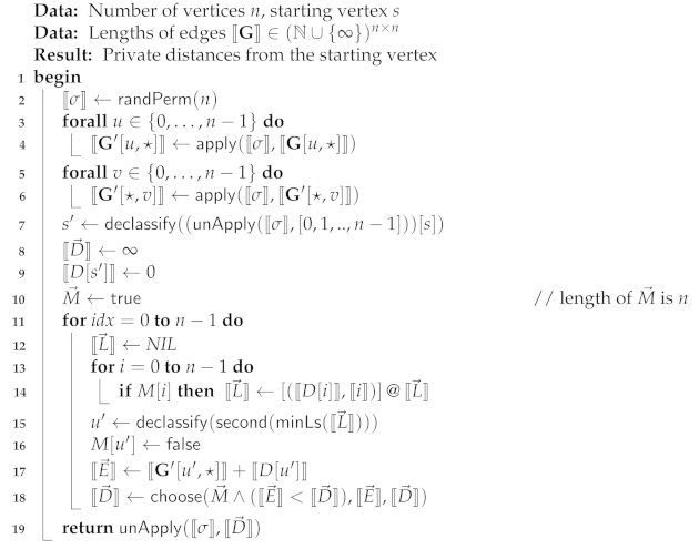
Dijkstra’s algorithm relaxes each edge only once, in the order of the distance of its start vertex from the source vertex. The edges with the same starting vertex can be relaxed in parallel. The algorithm cannot handle edges with negative weights. As Dijkstra’s algorithm only handles a few edges in parallel, Laud’s parallel reading and writing subroutines will be of little use here. Instead, we opt to use the dense representation of the graph, giving the weights of the edges in the adjacency matrix (weight “∞” is used to denote the lack of an edge). Our privacy-preserving implementation of Dijkstra’s algorithm is presented in Algorithm 5.
The main body of the algorithm is its last loop. It starts by finding the unhandled vertex that is closest to the source vertex. The mask vector indicates which vertices are still unhandled. The index of this vertex is found by the function given in Algorithm 6, which, when applied to a list of pairs, returns the pair with the minimal first component. We call with a list where the first components are current distances, and the second components are the indices of vertices. In non-privacy-preserving implementations, priority queues can be used to find the next vertex for relaxing its outgoing edges quickly. In privacy-preserving implementations, the queues are challenging to implement efficiently due to their complex control flow. Hence, the next vertex is found by computing the minimum over the current distances for all vertices not yet handled.
| Algorithm 5: Dijkstra’s algorithm |
![Cryptography 05 00027 i005]() |
| Algorithm 6: minLs: computing the pair with the minimal first component |
![Cryptography 05 00027 i006]() |
Algorithm 5 declassifies the index of the unhandled vertex closest to the source vertex. This declassification greatly simplifies the computation of , where the current distance of is added to the length of all edges starting at . Without declassification, one would need to use techniques for private reading here, which would be expensive. Note that both the computations of and take place in a SIMD manner, applying the same operations to , , , and for each .
This declassification constitutes a leak. Effectively, the last loop declassifies in which order the vertices are handled, i.e., how are the vertices ordered concerning their distance from the source vertex. Such leakage can be neutralized by randomly permuting the vertices of the graph before that last loop [
9]. In this way, the indices of the vertices, when they are declassified, are random. The declassification would output a random permutation of the set
, one element at each iteration.
The computation of this random permutation takes place at the beginning of Algorithm 5. We first generate a private random permutation for n elements. We will then apply it to each row of ; the application takes place in parallel for all rows. Similarly, we apply it to each column. Such permutation also changes the index of the source vertex, and we have to find it. We find it by taking the identity vector of length n, applying to it the inverse of , and then reading the position s of the resulting vector. Note that we declassify only the position s at this time, not the entire vector. At the end of the computation, we have to apply the inverse of to the computed vector of distances.
Dijkstra’s algorithm is used as a subroutine in certain APSD algorithms (
Section 3.2.1). Hence, we have also implemented a
vectorized version of Algorithm 5 that can compute the SSSD for several
n-vertex graphs simultaneously. Below, we call this version of the algorithm
. Obviously,
and
have the same round complexity. In contrast, the bandwidth usage of the latter is
n times of the former (when finding SSSD for
n graphs at the same time). In our empirical evaluation, we have benchmarked both versions of the algorithm.
3.1.4. Complexity of Algorithms
Two kinds of communication-related complexities matter for secure multiparty computation applications in the sense that these may become bottlenecks in deployments. First, we are interested in the bandwidth required by the algorithm, i.e., the number of bits exchanged by the computation parties. Second, we are interested in the round complexity of the algorithm, i.e., the number of round-trips that have to be made in the protocol implementing that algorithm.
Let n denote the number of vertices and m the number of edges of the graph. We assume that m is between n and , meaning that is and is . We also consider the size of a single integer (used as the length of an edge or a path or as an index) to be a constant. In this case, the steps of the Bellman–Ford algorithm (Algorithm 1) before the main loop require bandwidth and rounds. Indeed, both -statements have this complexity, while the complexity of is dominated by the sorting of n private values.
Each iteration of the main loop of Algorithm 1 requires bandwidth and rounds, with (Version 1) being the only operation working in non-constant rounds. The number of iterations is ; hence, the total bandwidth use is , in rounds. However, the number of iterations reflects the worst case, which has to be taken only if no further information is available. If we know that the SSSD algorithm will be called in a context, where the shortest path(s) we’re interested in consist of at most edges, then the iterating can be cut short, such that the algorithm only uses bandwidth in rounds.
One iteration of the main loop of Dijkstra’s algorithm (Algorithm 5) requires bandwidth and rounds, with being the only operation working in non-constant rounds. The entire loop thus requires bandwidth and rounds. The shuffling of rows and columns before that loop also requires bandwidth, but only constant rounds.
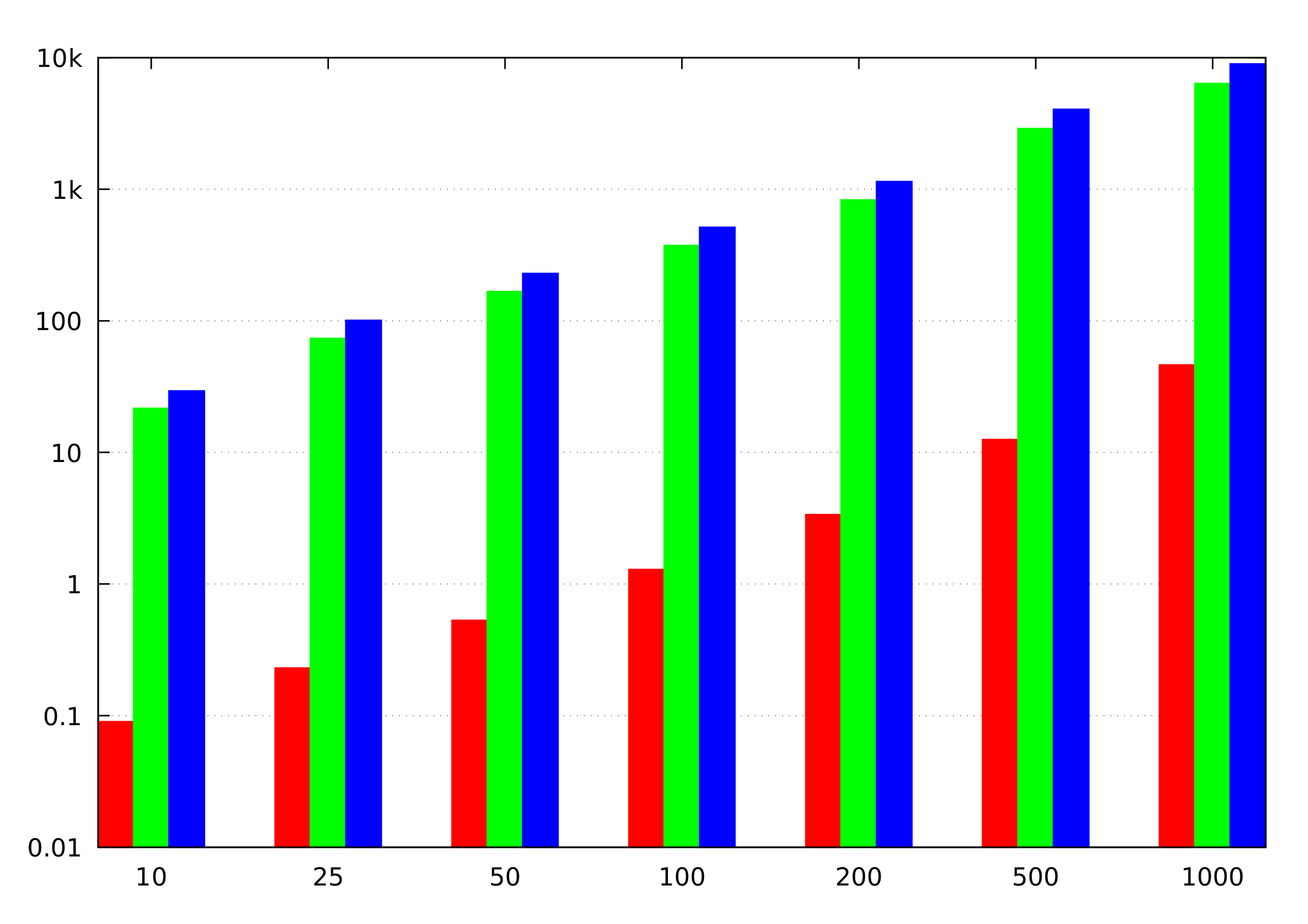
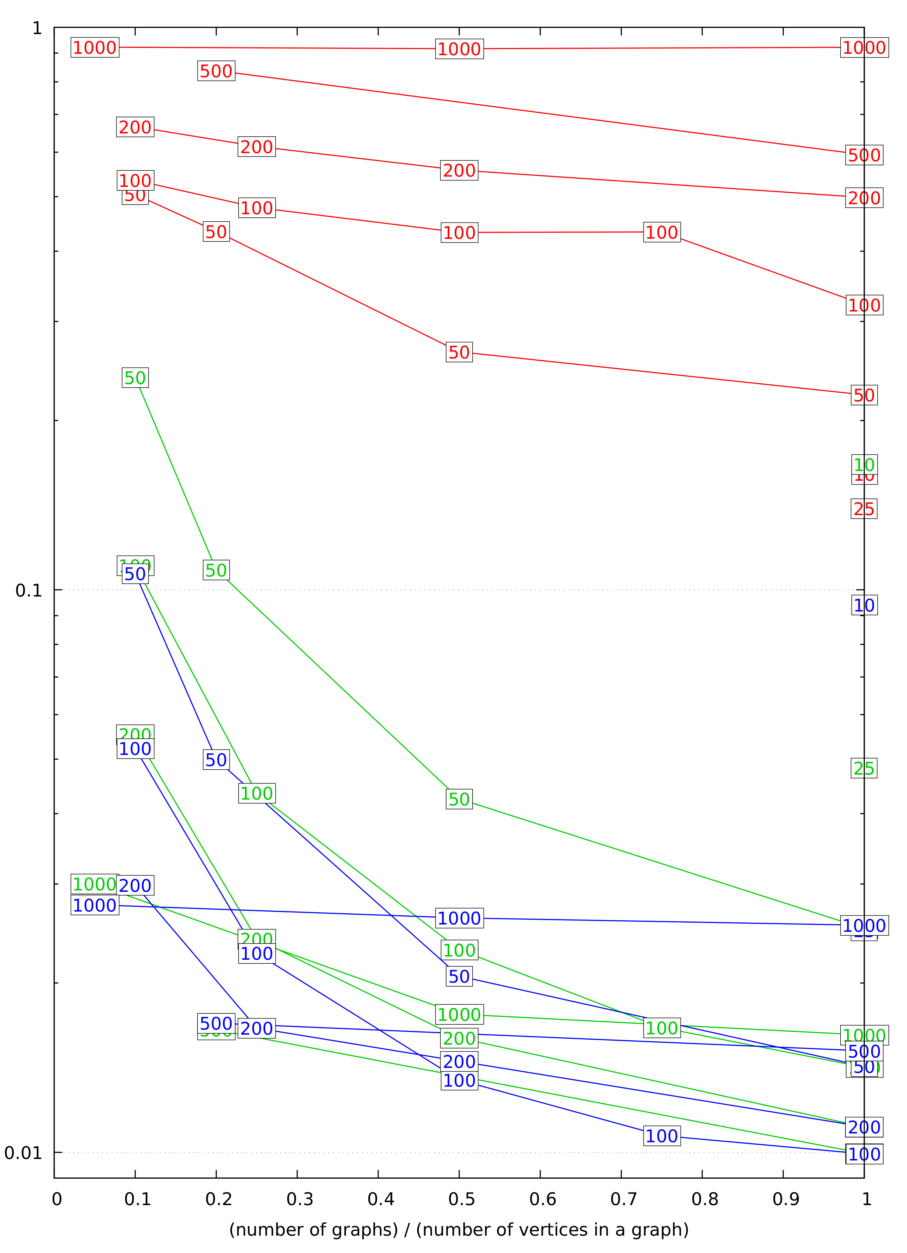
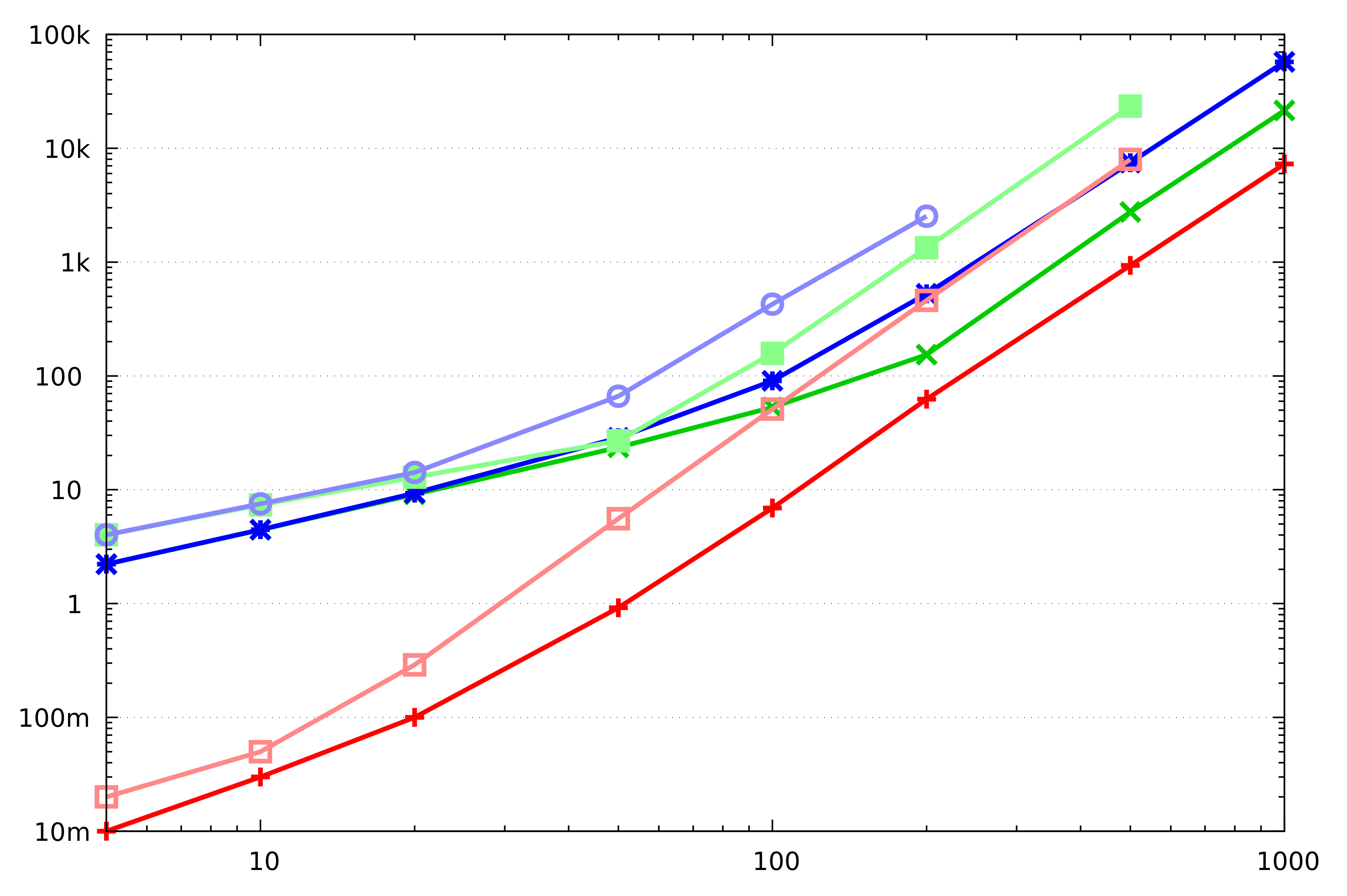
We see that Dijkstra’s algorithm requires less bandwidth than Bellman–Ford’s. Indeed, our benchmarking results (
Section 3.6) confirm that. The Bellman–Ford algorithm should still be considered attractive if we can limit the number of iterations it makes. Such limitations may stem from the side information that we may have about the graph, implying that shortest paths do not have many edges. A limited number of iterations is also possible if, at the end of each iteration, we compare the current vector of distances
with its value at the previous iteration, and stop if it has not changed. This leaks the maximum number of edges on the shortest path from the given vertex; perhaps this leak can be tolerated in some scenarios. The running time of Dijkstra’s algorithm cannot be limited in such a manner.


