Abstract
Traditionally, life has been thought improbable without assuming a special principle, such as vital power. Here, I try to understand organization of living systems in terms of a more rational and materialistic notion. I have introduced the notion of inhomogeneity, which is a novel interpretation of “negentropy”, and equivalent to “bound information”, according to the probabilistic interpretation of entropy. Free energy of metabolites is a labile inhomogeneity, whereas genetic information is a more stable inhomogeneity. Dynamic emergence can result from the conflict between two inhomogeneities, one labile and another stable, just like dialectic synthesis results from the conflict between thesis and antithesis. Life is a special type of dynamic emergence, which is coupled with reproduction mediated by genetic information. Biological membrane formation is taken as an example to formulate self-organization of biological systems through dynamic emergence. This system is ultimately driven by the Sun/Earth temperature difference, and is consistent with an increase in probability in the world. If we consider all entropy production related to life, such as degradation of materials and death of organisms, and ultimately the cooling of the Sun, probability always increases with the progress of living systems.
Keywords:
biological membrane; entropy; inhomogeneity; life; lipid; photosynthesis; probability; self-organization 1. Introduction
Life has long been a subject of continuing quests of philosophers and scientists. From the age of ancient Greek philosophy, distinction between living beings and non-living things has been an essential enigma that philosophers tried to answer. A simple and clear solution was to assume a special principle in living beings, as was introduced by Aristotle under the notion of “psyche” or “anima” [1]. Various different kinds of anima were supposed to characterize different kinds of living beings, such as plants, animals, and humans. Although Aristotle’s notion of “anima” seemed non-scientific or pre-scientific, we might be able to consider “anima” as a principle of life rather than a special force of life. In the nineteenth century, supporters of vitalism supposed a special force that drives life in cellular activity, morphogenesis, and reproduction. It was called either “vital force,” “Lebenskräfte,” or “Entelechie,” among others [2]. “Élan vital” of Henri Bergson [3] was sometimes confused with vital force, but could have meant something different [4]. Garrett [2] called recurrence of a conflict between vitalism and emergent materialism “intellectual amnesia.”
Various properties are used to characterize life: controlled metabolism, sensibility, self organization of cell and body structure, reproduction, autonomy, and consciousness. These are only representatives of many qualifications of life. Mechanistic understanding could be possible for some of these, such as metabolism, sensibility, reproduction, and autonomy. Obviously, we cannot find a plausible explanation of consciousness in the current status of understanding, although efforts to naturalize consciousness continue [5]. In addition, self-organization is a curious property of life that we cannot easily provide a mechanistic or materialist answer, because it is different from crystallization of minerals or self-assembly of bacteriophages and ribosomes, which are stabilizing reactions that occur spontaneously. Self-organization of living beings is a dynamic process that requires free energy and information, which was discussed from the viewpoint of “molecular vitalism” [6]. Apparently, it proceeds spontaneously, but it is an important aspect of life and a part of a vital process that needs explanation. In the present article, I will discuss self-organization of living beings in the light of dynamic emergence, which involves conflict of two inhomogeneities and production of emergent inhomogeneity. The notion of inhomogeneity [4] is related to entropy and information, but also probability. Probabilistic interpretation of entropy and information [7] is used to understand life in terms of inhomogeneity and dynamic emergence.
2. Inhomogeneity and Emergence
Self-organization of living systems, such as cells, organisms, and ecosystems, is explained by ingestion of “negative entropy” by Schrödinger [8] in the middle of the 20th century. Since then, various different versions of formulation were proposed, but the essential point remained identical, namely, that free energy flow into the living systems is coupled with dissipation of entropy to the outer world. Free energy is equivalent to negative entropy, and entropy increase is equivalent to realization of a more probable state. In other words, self-organization of living systems is part of a transition to a more probable world. In the following arguments, I intend to rationalize this apparently paradoxical statement by presenting realistic explanation using examples based on current biological knowledge.
I have introduced “inhomogeneity” I, which is defined as the “entropy deficit” or difference between the maximum entropy Smax and the actual entropy S [4]:
I = Smax − S.
Historically, inhomogeneity is equivalent to “bound information” of Brillouin [9], who also used “negentropy” for what I call inhomogeneity. I prefer inhomogeneity, because this term adequately describes the situation in which something is not distributed evenly. This is equivalent to the situation in which entropy is lower than the maximum possible entropy. The relationship between inhomogeneity and probability is simply illustrated in an example of binomial distribution (Figure 1).
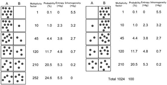
Figure 1.
Uneven distribution is evaluated by inhomogeneity and probability.
Let us consider a box with two parts, A and B. There is a virtual wall between the two parts, but there is no real obstacle that prevents movement of particles between the two parts. If ten particles are present in the box, and the particles can displace freely, under this circumstance, we can imagine 11 different states in which part A contains different numbers of particles. The multiplicity factor W(n) of each state, or the number of different combinations of identical but distinguishable particles, can be obtained by a simple calculation:
where n is the number of particles in A. Since the total number of W(n) (0 ≤ n ≤ 10) is 1024, the probability pn of each state is given by:
W(n) = 10!/n! (10 − n)!,
pn = W(n)/1024.
We find that pn is the largest when n = 5, namely, if an equal number of particles are partitioned in A and B. This probability is valid if the particles are freely displaced in the box, and the displacement is rapid enough for the time scale of measurement. We can also calculate entropy Sn of arrangement n:
where kB is the Boltzmann constant, and “ln” represents natural logarithm. This entropy calculation is similar to that used in the Boltzmann distribution of electron configuration (see e.g., Figure 4.2 in [10]). In this very simple example, Sn is also the largest (Smax = 5.5 kB) when n = 5, with an even distribution. Inhomogeneity of each state is given by Equation (1), and we find that inhomogeneity is maximal when the distribution is the most uneven, namely, all particles are localized in either part. Although this is a simple example, we can extend a similar estimation of probability and entropy in more complicated systems in which the number of parts is larger or the number of particles is larger. In another extension, we may suppose uneven probability qni of microstates i realizing a single macrostate n shown in Figure 1. In this case, the entropy Sn of this macrostate is given by:
where summation is calculated for all i. Equation (5) is the common formula of entropy calculation [9], which is reduced to Equation (4) if all qni are identical for all i. By this simple example, we can understand that entropy is maximal when the probability is maximal. If various macrostates are freely and rapidly interchangeable, the state of even distribution is the most probable, and the entropy of the system is maximized. In this example, the value of W(n) has a broad peak around the even distribution, but with larger number of total particles N, the binomial distribution will be approximated by a normal distribution, having a half width proportional to N1/2, and therefore, the distribution will have a relatively sharper peak at the even distribution (relative width N−1/2). This is just a case of the Principle of Maximum Entropy (PME) [10].
Sn = kB lnW(n),
Sn = − kB ∑ qni ln(qni),
Various forms of inhomogeneity are found in nature. Pressure of a gas or osmosis is a result of uneven distribution of molecules. Potential energy in gravitational, electric, or magnetic field may be a form of inhomogeneity due to concentration of energy, although we cannot say exactly where the energy is localized (tentative assumed to be in the target material). Internal energy of a chemical is also a form of inhomogeneity due to energy concentration within the molecule. All these forms of inhomogeneity are quantitatively expressed in terms of free energy, which produces entropy upon its release (see Equation (6) in Section 3.1).
In terms of inhomogeneity, we may formulate that inhomogeneity tends to decrease spontaneously. But we have to remember the essential premise of the problem, namely, that all states in Figure 1 can be exchanged freely and rapidly within the time scale of observation, as in the Boltzmann distribution of electronic states [10]. The same is true for various other cases described in the previous paragraph. Therefore, some inhomogeneity decays rapidly, whereas some other inhomogeneity such as nucleotide sequence of DNA remains fairly stable [11].
Inhomogeneity is defined with a fixed reference to a certain state of “maximum” entropy (Equation (1) and Figure 1). This is important, because any system can be made infinitely homogeneous, if we decompose materials, molecules, atoms, etc., and mix them thoroughly. Nevertheless, we have to consider a plausible final state after any change. The final state of “maximum” entropy cannot be determined without judgment of an observer. This depends on the physical and time scales of the phenomenon that we are analyzing. For example, when we are analyzing a biological system, we do not consider nuclear reaction that could happen under extensive radiation in a reactor. In contrast, we are not satisfied with our daily activity of sleeping, walking, and talking, to analyze the origin of biological organization. We have to determine the level of analysis to find an appropriate value of “maximum” entropy. In the analysis of biological organization that we are interested in, we should focus on biochemical activity of cells, and in cases, interaction of cells and organs depending on target of analysis. In such analysis, it is best to consider free energy of biochemical reaction as a principal source of inhomogeneity. Additionally, genetic information will have to be taken into consideration.
3. Inhomogeneity in Biological Systems
3.1. Free Energy in Biochemical Reactions
Decay of inhomogeneity often occurs spontaneously and serves as a driving force for various living and non-living processes. Biochemical free energy is a form of inhomogeneity. Note that energy itself is conserved upon any change, either a physical or chemical one. It is free energy but not energy that can drive changes. We can say that the entropy term of free energy represents the extent to which atoms, particles, or energy can be potentially dissipated. If many atoms are restricted to be bound within a molecule, configuration entropy (entropy of distribution in the sense shown in Figure 1) is decreased. A “high-energy” molecule such as ATP (adenosine triphosphate) harbors inherent instability (repulsion of negative charges in proximity), and thus keeps excess energy within its structure. Both of these are potential sources of driving force for chemical reactions by releasing free energy or dissipating entropy, if an appropriate reaction route is provided by a catalyst or an enzyme. In this way, biochemical reactions proceed spontaneously in the direction of decreasing free energy. Each enzyme contributes to the reduction of activation energy of the reaction in which it is involved, but the direction of reaction is governed by free energy change, namely, the difference in free energy of the reactants and products. Free energy change ∆G (under a constant pressure) consists of two terms, enthalpy change ∆H and entropy change ∆S of the reaction system. According to the formulation of Atkins [12]:
−∆G/T = −∆H/T + ∆S.
The first term of the right side of Equation (6) describes dissipation of reaction heat, or the entropy increase in the world (outside the system), and the second term is the entropy production in the system. The latter represents a decrease in the extent of concentration of particles and energy within the molecules involved in the reaction. Therefore, the left side of Equation (6) is the total increase in entropy, or ∆Stotal. In other words, free energy change (divided by temperature) is a measure of entropy increase in the entire world (system plus outside world). A biochemical reaction proceeds by consuming free energy and producing ∆Stotal (≡ −∆G/T).
The relationship between free energy and inhomogeneity is more clearly formulated by using the notion “affinity” A as used in the Belgian school of thermodynamics (see Chapter 4 in [13]). Affinity is defined as the difference between the total chemical potentials of products and reactants. Note that chemical potential is partial molar free energy. Therefore, affinity is a measure of the state of chemical system, in which affinity becomes zero at the equilibrium. Entropy production rate is expressed by using affinity as follows [13]:
where dξ/dt is the reaction rate. In this formulation, (A/T) is the driving force of the reaction, which corresponds exactly to the notion of inhomogeneity. However, because affinity is ultimately a derived notion of free energy, we consider free energy (or free energy change) as inhomogeneity in the following text for simplicity.
dS/dt = (A/T) dξ/dt,
3.2. Dialectics in Dynamic Emergence
Several models may be presented for self-organization without vital force. A simple model is a stick pile in a river stream (Figure 2A). Depending on the flow rate and the shape of the pile, turbulence with complex eddies is created. The driving force is the flow of water blocked by the pile. This is a conflict between two inhomogeneities: water flow is a directional movement of water, whose momentum is a directional inhomogeneity; a pile stuck in a river is a stable structure, which is an organization inhomogeneity. The former is a labile inhomogeneity, whereas the latter is a stable inhomogeneity. The conflict between the two inhomogeneities yields turbulence, which is another kind of inhomogeneity. Turbulence may be regarded as a kind of inhomogeneity involving complex, organized water flow. The formation of turbulence is characterized as an organization driven by the conflict between two inhomogeneities. The formation of this new kind of inhomogeneity is called “emergence” here. This definition of emergence removes any mysterious appearance associated with the term. The process is dynamic, because continuous flow of water is necessary for the formation of turbulence. This is a very simple example of dynamic emergence (Figure 3).
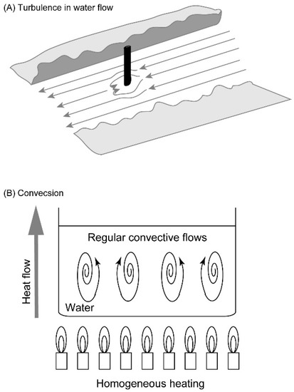
Figure 2.
Turbulence and convection as examples of emergence. (A) Turbulence in water flow blocked by a stick pile. (B) Convection of water in a casserole heated evenly. These images are just schemes for explanation, but not based on observation.
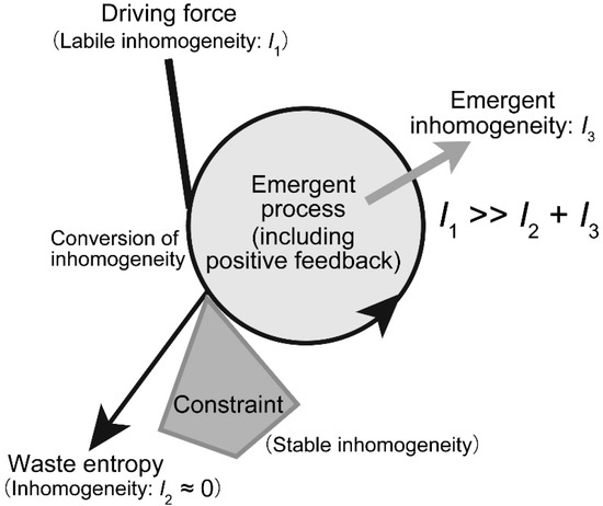
Figure 3.
Schematic model of dynamic emergence. In dynamic emergence, a conflict between two inhomogeneities, one labile and another stable, produces another kind of inhomogeneity. At the same time, the process produces a large amount of entropy, which corresponds to the decrease in labile inhomogeneity. In most cases, the process includes positive feedback, which is the direct origin of the emergent inhomogeneity. The amount of emergent inhomogeneity is much smaller than the amount of consumed inhomogeneity.
Convection is another example of dynamic emergence (Figure 2B). If the water is warmed at the bottom of the casserole, convection occurs spontaneously. Typically, the convective flow is organized in a form of honeycombs. Prigogine called this “dissipative structure,” because structured flow is formed at the expense of entropy dissipation [13,14]. This can also be described in our framework of dynamic emergence. Heat is a form of labile inhomogeneity that serves as a driving force, while gravity is another form of inhomogeneity, which is not labile. Convective structure is dynamic, because it stays as long as heat is provided. We call it emergence, because convection is an inhomogeneity different from heat and gravity.
Dynamic emergence may be viewed as a dialectic process. In Hegelian dialectics, the conflict between the thesis and the antithesis will be resolved into synthesis by the action of “Aufheben.” This dialectic was introduced to explain changes in ideas during the long history of human culture. Hegel did not exactly explain the action of Aufheben. Nevertheless, we can apply a similar framework of explanation to our dynamic emergence (Figure 3): The conflict between the two different inhomogeneities will be resolved by the emergence of a new kind of inhomogeneity. Dynamic emergence is certainly different from the Hegelian dialectic, because, in our framework, inhomogeneity is associated with material support. It is not an abstract idea or mental activity. Dynamic emergence has a physical or material basis underlying it. The emergence is not a miracle or something supernatural. We can give a perfect physical explanation of dynamic emergence. I use the term emergence to focus on the novelty of inhomogeneity that is produced from the conflict between the two original inhomogeneities. Many authors tried to understand natural phenomena and life in terms of “emergence” [15,16,17,18,19]. A common usage of the term is to denote something happening from complex interactions. But complexity is not an explanatory notion. In addition, precise and quantitative measure of emergence has not been provided in the analysis of emergence created by complexity. The dynamic nature of emergence should be emphasized here. We apply the notion of dynamic emergence to biological systems in the following sections.
Before proceeding, however, I have to explain possible roles of chaos in dynamic emergence. Complex systems sometimes show chaotic behavior, in which apparently random states of disorder is governed by essentially deterministic laws (see, for example, Section 2.3 in [20]). This could be the origin of variable outcome in dynamic emergence. In the actual biological systems, variability is kept to minimum, but the possibility of chaotic behavior could be a source of novelty or evolution. This is an interesting point, which we will have to develop in the future.
3.3. Role of Genetic Information
Understanding the nature of genetic information is essential to formulating the dynamic emergence of biological systems. An organism is reproduced by the action mediated by genetic information, whose expression leads to synthesis of biological molecules and cell structure. In this respect, genetic information appears to be specific to biological systems. However, we can imagine a non-living system that has a little but significant information. Using convection as an example again, just imagine a situation in which we repeat convection experiments. Eventually, the bottom of the casserole will rust. Then, the rust could act as an initial trigger that induces fluctuation within the water to promote convection, which is otherwise caused by very small fluctuations within the water. The rust could be part of the information that initiates convection at the same location each time. This primitive information could be a model of genetic information in living systems, in which biological activity promotes the replication of genetic material, which will direct the biological activity in the next round. We certainly recognize a clear difference between the rust on the bottom of casserole and the genetic information encoded by genomic DNA. The former gives just a single bit of information, but genetic information is more complicated with four bases. Rust does not have a specific recognition system that characterizes the genetic information. Nevertheless, the rust model provides the fundamental basis for genetic information in biological systems.
Now, we inspect the nature of genetic information (Figure 4). The information of DNA is encoded by four nucleotides, A, T, G, and C. Genetic information is often understood in terms of nucleotide sequence of a gene or a coding sequence. Here, we consider a gene as a set of a regulatory sequence and a coding sequence (or a set of exons). However, a gene can start anywhere within the genome if steric or structural restrictions, such as telomere or centromere, are not imposed. Therefore, information content should be considered for each gene, rather than calculated as a deviation from a random sequence. To calculate information content of a gene, we first focus on a single nucleotide within a conserved gene. Information content depends on whether the site is highly conserved or more variable. For a single site of DNA, average information content H is given by the following formula:
where pi is the probability of nucleotide i (i = A, T, G, or C). This gives the extent of variation of nucleotides, and corresponds to entropy as defined in Section 2. Note that H is not itself the actual content of genetic information. Average information content is also known as “information entropy” [21]. H and S are different in unit and calculation method, but both are supported by probability behind them. As shown in Figure 1 in Section 2, both values are the largest when the probability is the highest. This is shown by the probabilistic interpretation of entropy [7] and is consistent with the PME [10]. If each nucleotide is expected to occur at an identical probability (Figure 4A,B), the average information content is 2 bits. In other words, the information gain of knowing the nucleotide is 2 bits. This is the logically possible, maximal value of information content at a single site. However, the actual probability is not evident. In a typical estimation in bioinformatics [11], average nucleotide composition of a gene or a genome is used as probability of nucleotide at each position. In this case, the value of average information content is identical over all sites of the entire gene or entire genome, and this is the maximum value of information entropy Hmax.
H = −∑ pi log2(pi),
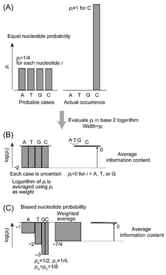
Figure 4.
Graphical explanation of average information content of DNA. (A) Plot of equal probability. (B) Logarithmic plot of equal probability. (C) Logarithmic plot of unequal probabilities at a partially conserved site. In this case, the inhomogeneity or information content of the site is 1/4.
If we take a single nucleotide sequence, such as a human gene sequence, we are not able to evaluate the information content of the sequence. Using phylogenetic data, a large number of homologous sequences are used to construct a multiple alignment. Occurrence of each nucleotide is calculated for each site and used as the probability of the nucleotide for this site. For a highly conserved site, only a single nucleotide might be found in all sequences. For a neutral site, the four nucleotides might occur at an average frequency. Figure 4C depicts an intermediate situation. The average information content determined with this set of probabilities H is a measure of extent of permitted variability. It is used to estimate the actual information content harbored by the site which is again called inhomogeneity I.
I = Hmax − H.
By summing up all values of I over a single gene, we can estimate the inhomogeneity or the information content of the gene. A similar value of information can be calculated for an amino acid sequence. Genetic information is, therefore, relative to the available sequence data. This is the limit of current status of bioinformatics. Theoretically, information content could be calculated by functional constraint of enzyme, but it is not feasible at present.
Genetic information can be considered as a stable inhomogeneity, as long as the genomic sequence is maintained by highly conservative, high fidelity replication and repair systems. Genetic information conferred to each enzyme is also stable during the catalytic reaction. Genetic information of DNA and enzymes is not absolutely unchangeable, but can be changed during the process of mutation and genetic drift. Nevertheless, we can imagine that the inhomogeneity of a gene or an enzyme does not vary a lot unless its function is fundamentally altered.
3.4. Dynamic Emergence in Biological Systems
3.4.1. Inhomogeneities in Biology
The two classical examples of non-living systems in Section 3.2 give us a hint of dynamic emergence in living systems. We have to consider two major types of inhomogenetity in life: free energy of metabolites and genetic information of DNA (and RNA and proteins). However, the ultimate source of metabolic free energy is the sunlight, or more precisely, the temperature difference between the Sun and the Earth, or inhomogeneity of temperature. This is the essential point to understand in explaining life and biosphere. Schrödinger did not understand the importance of photosynthesis when he formulated the notion of negentropy in explaining biological activity in 1944 [8], because the mechanism of photosynthesis was uncovered later in the 1950s and 1960s. The first experiment of photophosphorylation was performed by Arnon et al. [22], and the basic mechanism of oxidation-reduction reactions induced by the photosynthetic reaction centers was proposed by Hill and Bendall [23]. Schrödinger [8] was able to explain the life of heterotrophs, but the life of plants and the food chain remained unexplained. Genetic information of DNA, bioenergetics of mitochondria and chloroplasts, and morphogenesis, all these essential notions of biology were unraveled in the 1960s or later. Unfortunately, fundamental understanding of these in terms of entropy or inhomogeneity remained obscure until recently, or even now.
3.4.2. Hierarchy of Emergent Processes in Biology
I have formulated various biological processes in terms of inhomogeneity in a previous paper [4]. In many bioenergetic processes, the free energy of incoming metabolites is an inhomogeneity to be degraded, and the metabolic pathway consisting of various enzymes functions as a stable inhomogeneity that determines the fate of metabolites. The conflict between these two kinds of inhomogeneities results in a new kind of inhomogeneity, which is characterized as an emergence. In photosynthesis, temperature difference of Sun/Earth is the incoming inhomogeneity, which is then converted to an inhomogeneity of reductant/oxidant pair, or an inhomogeneity of excess/deficit of electrons, via a conflict with the photosynthetic electron transfer pathway located in the thylakoid membranes of chloroplasts and cyanobacteria (Figure 5A). The reducing power of the initial reductant NADPH (reduced form of nicotinamide adenine dinucleotide phosphate) is then transferred to sugars, whereas the oxidant remains oxygen, which has filled an important part (currently 21%) of the atmosphere since more than 2 billion years. Atmospheric oxygen is entirely the product of past photosynthesis of plants, algae, and cyanobacteria. In the metabolism of heterotrophs, the reductant is supplied as food, whereas the oxidant is supplied from the air. The same is true for nonphotosynthetic tissues of plants. Figure 5A is presented for the understanding of the entire biosphere. If some readers tend to find the situation in heterotrophs, it is shown in Figure 5B. But it is my intention to understand the whole biological world in a single scheme like Figure 5A, including all processes of life in an integral network. This network may be completed within a single photosynthetic organism, but it is also realized in the whole biosphere, if we do not consider individual cells and organisms separately.
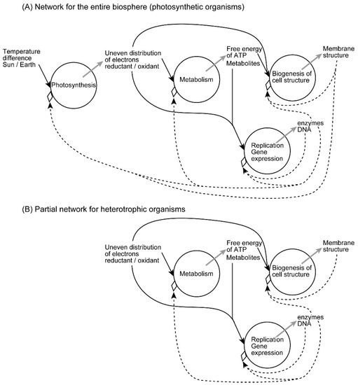
Figure 5.
Hierarchy of the network of emergent processes in biological organization. (A) Network of the entire biosphere, valid also for photosynthetic organisms. (B) Network of heterotrophic organisms. Each circle represents an emergent process, in which one or more incoming inhomogeneities are shown by black arrows, whereas an emergent inhomogeneity is shown by a grey arrow. Inhomogeneities acting as constraints are shown by dashed arrows. Note that the constraints are not inhibitors. Rather, they also contribute to the emergence. In the entire biosphere, the ultimate driving force is provided by the sunlight, and various positive feedback loops enable self-organization of cell structure. The network is not closed within a single organism, but extends over the entire biosphere including various organisms. However, the constraints work only within a single cell or an organism. Heredity and evolution are not explicitly included in this scheme, which may be extended to include them as shown in [4]. The network in (A) is applied for the entire biosphere, but it is also valid for photosynthetic organisms, although excess reductants and oxygen are released for consumption by heterotrophs. In the partial network of heterotrophic organisms, incoming inhomogenetities are food and oxygen, which represent reductant and oxidant, respectively.
In the metabolic processes in heterotrophs (and nonphotosynthetic tissues of plants), the incoming inhomogeneity is the reductant/oxidant pair (sugar/oxygen), and the emergent inhomogeneity is the chemical power of ATP and other high-energy metabolites. The metabolic pathways serve as a stable inhomogeneity. In each of photosynthesis and bioenergetic processes, we might be able to imagine simply a chain of biochemical reactions, rather than an emergent process. But the reaction chains are highly ordered with elaborate enzymes under fine regulations. All these require a large amount of information, which is ultimately encoded by the genomic DNA. The information is a kind of inhomogeneity, which selects substrates to process, and directs biochemical reactions to occur. Biochemical reactions are often compartmentalized within a cell according to the information conveyed by the protein sequence. We should bear in mind the equivalence of information and inhomogeneity [4]. In this sense, genetic information is an inhomogeneity that directs the flow of free energy of metabolites, through the realization of metabolic pathways with highly selective, and highly efficient, and well-localized enzymes. Each metabolic substrate, in general, bears a high free energy, which tends to decay if a reaction pathway is present. Nevertheless, every metabolic substrate is stable enough in its own. It is subject to a biochemical reaction if an appropriate enzyme is provided. Each enzyme holds information necessary for selecting a substrate, and directing a precisely determined reaction. In this sense, any enzyme is an inhomogeneity that act as a constraint. These reflections lead us to view metabolic processes as emergent processes resulting from the conflict between two different inhomogeneities, namely, free energy of metabolites and genetic information. We should not forget, however, that both kinds of inhomogeneities have probabilities behind their entropic appearance. When a metabolic reaction proceeds, free energy decreases to achieve the final state with higher probability, if we take all resulting products and heat in consideration. Several reactions might be possible, but only one of them is selected by an enzyme. This is also a probabilistic process, in which genetic information conferred to the enzyme is used. The conflict between labile and stable inhomogeneities is an origin of emergence, the formation of a new kind of inhomogeneity.
Theoretically, the distinction between labile and stable inhomogeneities in dynamic emergence might not be inherent in the substances involved in the process. A single substance can be a driving force and constraint in different processes. An enzyme is itself a polypeptide, which can give metabolic free energy when degraded. But an enzyme acts as a constraint in determining the metabolic pathways. Nucleotides may also act as metabolic energy and constraint. The two types of inhomogeneities should be identified for individual processes. Note that I use “type” and “kind” in qualifying inhomogeneity. Type refers to the distinction between labile/stable or driving force/constraint. Kind refers to the different entities that represent inhomogeneity, such as temperature, free energy, electron, information, etc. As explained above, each kind of inhomogeneity could be two types of inhomogeneity acting differently in dynamic emergence.
In biochemical reactions, however, the emergent inhomogeneity is still a form of free energy of metabolites. In this case, we may consider a complex network of metabolic pathways as a single emergent process that engenders a new kind of inhomogeneity, such as cellular structure. This is a morphogenic process that characterizes a part of biological self-organization.
4. Self-Organization in Living Systems
Self-organization of living systems is essentially understood as a dynamic emergence originating from the conflict between metabolic free energy dissipation (driving force) and genetic information (constraint). Membrane formation will be explained according to this scheme.
4.1. Lipid Bilayer Structure of Biological Membrane
Biological membrane consists of lipids and proteins, but it is amphiphilic lipids that form bilayer structure of biological membranes (Figure 6). A molecule is called amphiphilic if it has both hydrophilic and hydrophobic parts, and this is the essential point in organization of biological membranes. If amphiphilic lipid molecules, such as phosphatidylcholine and phosphatidylethanolamine, are placed in an aqueous environment, they will form spontaneously lamellar structure or micelles, depending on the size and nature of component hydrophilic and hydrophobic groups. Both lamellae and micelles are formed as a result of repulsion of hydrophobic groups and water. If the cross-sectional areas of the hydrophilic head group and the hydrophobic acyl groups are equal, then a planer structure called “bilayer” consisting of two layers of lipids will be formed, in which the hydrophobic groups of both layers faces to each other and the hydrophilic groups contact surrounding water molecules. The lipid bilayer is the standard basic structure of biological membranes, with protein molecules embedded within it. If the cross-sectional area of the hydrophilic head group is larger than that of the hydrophobic groups, such as the case in lysophosphatidylcholine (lacking an acyl group) and free fatty acid anion (common soap), spherical aggregates of lipids called micelles are formed, in which hydrophobic parts are centered, leaving the hydrophilic head groups facing the aqueous phase.
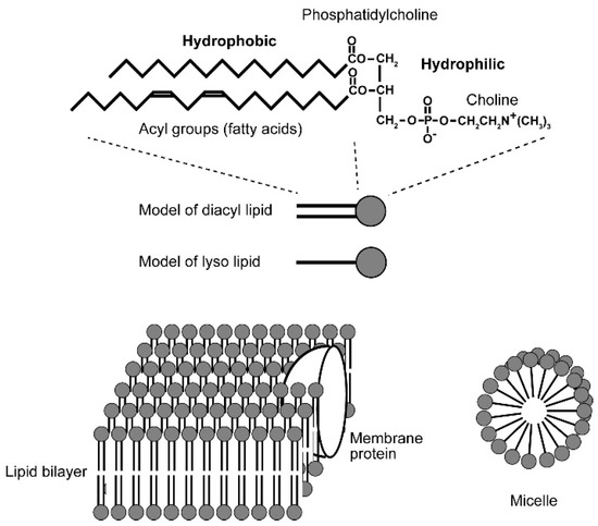
Figure 6.
Amphiphilic lipid molecule and organization of bilayer and micelle. Phosphatidylcholine is shown as an example of amphiphilic lipid. Any biological membrane is far more complicated, having various different kinds of lipids with different acyl groups. Lipid bilayer is a planer structure formed by two layers of lipids, in which the acyl groups of the two layers contact each other, whereas the hydrophilic head groups face the aqueous phase. A micelle is formed by lyso lipids lacking an acyl group or soap (fatty acid salt), in which the hydrophobic groups form the central core and the hydrophilic groups are exposed to the spherical surface and contact water.
Note that the formation of bilayer or micelle structure as explained above is a stabilizing process analogous to crystallization. This is a static organization but not a dynamic one, because we have already lipids and water in hand and mix them in a laboratory experiment. The situation is different in living organisms because lipids are synthesized within the membrane and inserted into the membrane in expanding membranes within a growing cell. Introductory biochemistry textbooks such as [24] will be helpful for the readers who are not familiar with biological membrane and lipids.
4.2. Biosynthesis of Fatty Acids and Lipids
In general, biological membranes are not synthesized from scratch. Each existing membrane within the cell is enlarged by incorporating additional lipid molecules within its bilayer. Cell division is a process of partitioning the enlarged membranes to daughter cells. Biological membranes contain amphiphilic lipids, but many metabolites are hydrophilic. When an amphiphilic lipid molecule is synthesized from its components, an excess free energy is necessary to accommodate it in an aqueous environment. Figure 7 shows a schematic pathway of fatty acid and membrane lipid biosynthesis. Fatty acids that form membrane lipids are called long-chain fatty acids, because they contain 14 or 16 methylene groups (-CH2-) as well as a methyl group (-CH3). Such fatty acid molecules are very hydrophobic. Nevertheless, fatty acids are synthesized by a soluble enzyme called fatty acid synthase using hydrophilic substrates. The growing chain of fatty acid is embedded within a hydrophobic pocket of a small protein called acyl carrier protein (or its equivalent within the large fatty acid synthase molecule, depending on organisms) to keep the hydrophobic molecule apart from the aqueous environment. Each step of fatty acid synthesis involves an extension of the acyl chain by two-carbon (C2) units, which is provided by malonyl Coenzyme A (CoA). The reaction is accompanied by a release of a carbon dioxide molecule, which is an entropy dissipating process. Malonyl CoA is synthesized from acetyl CoA by adding carbon dioxide, accompanied by the hydrolysis of an ATP molecule. After addition of the C2 unit, the carbonyl group is reduced to the methylene group by two molecules of NADPH, a powerful biological reductant. The reducing power of NADPH is conserved within the molecule of fatty acid, which is eventually used as a biological energy source when it is oxidized. In this sense, biological membranes are both structure and energy reserve (reserve of reductant). Therefore, the synthesis of a hydrophobic molecule, such as fatty acid, requires enormous consumption of free energy, or entropy dissipation, in other words, decay of inhomogeneity.
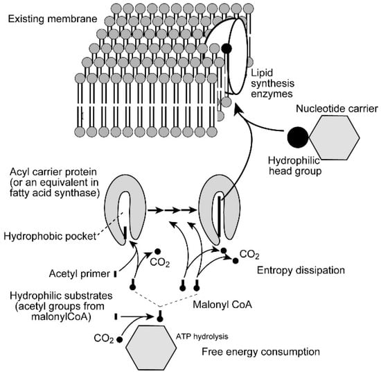
Figure 7.
Fatty acid synthesis and biosynthesis of biomembrane. Fatty acids in membrane lipids are composed of 16 or 18 carbon atoms (14 or 16 methylene groups plus methyl and carboxyl groups), and synthesized by condensing C2 units. The hydrophobic chain of growing fatty acid is encapsulated in the hydrophobic pocket of acyl carrier protein. The condensation reaction is performed with dissipating entropy in the form of carbon dioxide, originally attached to the C2 unit via hydrolysis of ATP. Reduction of acyl chain by NADPH is not explicitly shown in the figure. The synthesized fatty acid is transferred to glycerol phosphate in the membrane to form phosphatidic acid, which is then dephosphorylated to diacylglycerol. Hydrophilic head group is transferred to either phosphatidic acid or diacylglycerol (depending on lipid to synthesize) to form an amphiphilic lipid molecule. See text for details.
The protein part is removed when the acyl group is transferred to glycerol phosphate to make phosphatidic acid, which is then hydrolyzed to diacylglycerol. These are already incorporated into the membrane. A hydrophilic head group is provided as a precursor, in which a nucleotide carrier (cytidine diphosphate, CDP, or uridine diphosphate, UDP) binds the head group. Transfer of the head group to phosphatidic acid or diacylglycerol (depending on the kinds of lipids) produces an amphiphilic lipid molecule, an authentic member of the membrane. Hydrolysis of nucleotides (equivalent to ATP) is again required to build an amphiphilic lipid molecule. All these processes of lipid synthesis are catalyzed by respective enzymes, many of which are embedded in the membrane. Therefore, the site of lipid synthesis is already within the membrane.
In this way, the process of lipid biosynthesis consumes a large amount of free energy to produce an amphiphilic molecule and to embed it within an existing membrane. We can characterize this process as a dynamic emergence. The labile inhomogeneity that acts as a driving force is the free energy of ATP or equivalent nucleotides (needed to produce glycerol phosphate, the precursors of the hydrophilic part, and malonyl CoA) and the reducing power of NADPH (needed to synthesize fatty acids), and the inhomogeneity acting as a constraint is both biosynthetic enzymes and existing membranes within an aqueous environment. Enzymes determine which molecules are to be synthesized, whereas existing membranes provide sites of incorporation of synthesized lipid molecules. Both actions can be classified as inhomogeneities acting as constraints, because they select a single fate of the molecule among various probable ones.
4.3. Dynamism of Membrane Biogenesis
The fact that an existing membrane is enlarged by the action of lipid biogenesis is interpreted as a positive feedback driven by consumption of free energy. The feedback exerts in two ways: First, existing membranes are themselves basis of constructing and incorporating new lipid molecules; Second, the membrane structure allows cells to function as sites for metabolic processes, which provides necessary substrates for building lipid molecules. These two types of positive feedback support the dynamic emergence of biological membrane formation that looks like self-organization. In contrast to the formation of lipid bilayer in laboratory experiments, which is characterized as a static and stabilizing organization, biological membrane formation is a dynamic process characterized as an emergence. Membrane formation may be used as a typical example of self-organizing activities of cells or organisms. As a summary of this section, I repeat that self-organization of biological membranes and, therefore, the cell structure is a dynamic emergence resulting from the conflict between metabolic free energy (ATP and NADPH are different forms of inhomogeneities) and inhomogeneity constraint consisting of enzymes and the hydrophobic/hydrophilic environmental structure. This is also included in the scheme of the entire biosphere in Figure 5.
5. Problems Related to Inhomogeneity and Probability in Biological Systems
5.1. Evolution
In this short article, I do not try to describe details of organization of organism structure, and ecological structure, although I believe some kinds of dialectical processes or dynamic emergence are involved in these self-organization processes. Evolution is another aspect of dynamic emergence in biosphere (see [25] for an introductory textbook). Biological evolution is mainly a result of mutation and natural selection as far as selectable characters or nonsynonymous mutations are concerned. Changes and accumulation of silent or synonymous mutations are subject to a probabilistic process called genetic drift. Macroscopic or morphological changes could be explained by mutations in developmental switches according to the typical model of evolutionary developmental biology. In addition, speciation is sometimes characterized by the existence of genomic islands harboring mutational hot spots. The role of epigenetics and phenotypic flexibility is also argued.
Evolution may be viewed as a dynamic emergence resulting from the conflict between mutational diversification and competition of reproductive rates imposed by resource restrictions (see [26] for a comprehensive narrative). We can describe the traces of past evolution by either fossil comparison or phylogenetic reconstruction. But we cannot foresee future evolution, because we do not know exactly which mutations to occur and how selective pressures act on them. Even orthogenesis may not be predicted based on the past evidence of directed evolution. Preadaptation or exaptation is an explanation of the result of evolution, but not a predictive notion. Evolution looks adaptive because we are focusing on the organisms that have survived the past environmental changes. A thought experiment in which organisms never die suggests that evolution would not occur in such an immortal world. Evolution occurs because almost all organisms die without offspring. Only a small number of species succeeded in maintaining their lineages, which we characterize as having higher fitness. Therefore, evolutionary innovation is a result of vast extinction.
An objection to this statement could be that an organism with high plasticity might show an evolution by changing its property. This could be achieved by epigenetics or a huge genome equipped with various alleles that can be switched depending on the environment. This curious creature could survive environmental changes, and change its form each time. In this case, trait changes do not result from extinction. As a biological entity, however, this type of organism does not exist in nature, and is not a topic of evolutionary explanation. In addition, such a plastic organism does not change its genome after its adaptive changes in traits. Nevertheless, an idea or a cultural entity could survive infinitely in a flexible way, because such entity remains as a record even though it becomes unpopular. After some time, it will revive, like fashion trends.
Evolution may be viewed as a self-organization that contradicts the second law of thermodynamics claiming monotonous entropy increase. In fact, evolutionary innovation is compensated by the waste entropy of extinct organisms. Evolution is a process of entropy production, in which inhomogeneity of metabolic free energy (ultimately the Sun/Earth temperature difference) is degraded in conflict of spatial and environmental constraints that limit survival of organisms. If we focus on the survivors, then evolution appears as a creative process, but if we think of all dead creatures of the past, then evolution is a large-scale, destructive process, in which entropy increases, inhomogeneity decreases, and probability increases. The creative, organizing nature of evolution that we recognize in biology is an emergence resulting from such conflict between inhomogeneities. It is an entropy producing process in entirety, and the whole process of biosphere is directed to a world with a higher probability.
5.2. Probability of Life
Probability is, therefore, compatible with the existence of actual life forms, but we still do not know whether other forms of life are equally likely to exist. Jacques Monod wrote in 1970 that the probability of emergence of life was minute, and the existence of life on Earth, and even the existence of human beings, was a result of very rare chance [27]. Current astrobiology does not support this view, and supposes rather that we are only one of the probable forms of life, many of which are certainly present somewhere in the cosmos [28]. We agree with the astrobiologists, because decay of inhomogeneity might occur in various ways, and our living world might not be a unique one.
If life is defined as a principle of dynamic emergence coupled with reproducing ability with genetic information as described above, the type of life forms that we find on Earth may not be the only one. There could be various possible forms of life in the universe. Astrobiologists tend to search life forms that are similar, in some way, to the actual life forms on Earth. We are not sure if human-like creature exists somewhere in the universe. Nevertheless, the actual life forms are a consequence of the past dynamic emergence occurring on Earth. It is not possible to predict future life forms on Earth or possible life forms elsewhere in the universe.
6. Conclusions
Our initial question was whether organization of living systems is explained by probability. Various opinions in the past were rather negative to this question, namely, life has been thought improbable without assuming a special principle, such as vital power. In the present article, I introduced the notion of inhomogeneity, which is a novel interpretation of “negentropy” and equivalent to “bound information”. Relying on the probabilistic interpretation of entropy, we use inhomogeneity as a unified notion in physical chemistry and information science. There are two types of inhomogeneity, namely, labile and stable ones. Free energy of metabolites is a labile inhomogeneity, whereas genetic information is a more stable inhomogeneity. Then, I formulated three theses: First, labile inhomogeneity is the driving force of various phenomena in nature, and any decrease in inhomogeneity corresponds to an increase in probability. Second, the conflict between labile and stable inhomogeneities could result in dynamic emergence, producing a new kind of inhomogeneity through complex dynamics involving positive feedback. Third, life is a special kind of dynamic emergence coupled with reproduction mediated by genetic information. According to these considerations, self-organization of living systems, such as cells, multicellular organisms, and ecosystems, is a consequence of consumption of inhomogeneity, which results ultimately from the Sun/Earth temperature difference, and represents an increase in probability in the world. This seems to contradict with the common idea that the evolution of living systems is a rare, special phenomenon that contradicts the second law of thermodynamics asserting increase in entropy. However, if we consider all entropy production related to life, such as degradation of materials and death of organisms, and ultimately the cooling of the Sun, probability always increases with the progress of living systems.
Funding
This research received no external funding.
Institutional Review Board Statement
Not applicable.
Informed Consent Statement
Not applicable.
Data Availability Statement
Data sharing is not applicable.
Conflicts of Interest
There is no conflict of interest to declare.
References
- Aristotle. On the Soul. Parva Naturalia. On Breath; Hett, W.S., Translator; Loeb Classical Library 288; Harvard University Press: Cambridge, MA, USA, 1957. [Google Scholar]
- Garett, B. Vitalism versus emergent materialism. In Vitalism and the Scientific Image and Post-Enlightenment Life Science. 1800–2010; Normandin, S., Wolfe, C.T., Eds.; Springer Science-Business Media: Dordrecht, The Netherlands, 2013; pp. 127–154. [Google Scholar]
- Bergson, H. L’évolution Créatrice; Press Universitaires de France: Paris, France, 1907. [Google Scholar]
- Sato, N. Scientific élan vital: Entropy deficit or inhomogeneity as a unified concept of driving forces of life in hierarchical biosphere driven by photosynthesis. Entropy 2012, 14, 233–251. [Google Scholar] [CrossRef]
- Feinberg, T.E.; Mallatt, J. Consciousness Demystified; MIT Press: Cambridge, MA, USA, 2018. [Google Scholar]
- Kirschner, M.; Gerhart, J.; Mitchison, T. Molecular “vitalism”. Cell 2000, 100, 79–88. [Google Scholar] [CrossRef]
- Jaynes, E.T. Information theory and statistical mechanics. Phys. Rev. 1957, 106, 620–630. [Google Scholar] [CrossRef]
- Schrödinger, E. What is Life? The Physical Aspect of the Living Cell; Cambridge University Press: Cambridge, MA, USA, 1944. [Google Scholar]
- Brillouin, L. Science and Information Theory, 2nd ed.; Academic Press: New York, NY, USA, 1962. [Google Scholar]
- Grandy, W.T., Jr. Entropy and the Time Evolution of Macroscopic Systems; Oxford University Press: Oxford, UK, 2008. [Google Scholar]
- Mount, D.W. Bioinformatics; Cold Spring Harbor Laboratory Press: New York, NY, USA, 2001. [Google Scholar]
- Atkins, P.W.; de Paula, J. Elements of Physical Chemistry, 4th ed.; Oxford University Press: Oxford, UK, 2005. [Google Scholar]
- Prigogine, I.; Kondepudi, D. Thermodynamique. Des Moteurs Thermiques aux Structures Dissipatives; Odile Jacob: Paris, France, 1999. [Google Scholar]
- Nicolis, G.; Prigogine, I. Self-Organization in Nonequilibrium Systems: From Dissipative Structures to Order Through Fluctuations; Wiley International: New York, NY, USA, 1977. [Google Scholar]
- Nicolis, G.; Nicholis, C. Foundations of Complex Systems: Emergence, Information and Prediction, 2nd ed.; World Scientific: Hackensack, NJ, USA, 2012. [Google Scholar]
- Mainzer, K. Der Kreative Zufall. Wie das Neue in Die Welt Kommt; C. H. Beck: München, Germany, 2007. [Google Scholar]
- Holland, J.H. Emergence from Chaos to Order; Oxford University Press: Oxford, UK, 1998. [Google Scholar]
- Morowitz, H.J. The Emergence of Everything. How the World Became Complex; Oxford University Press: Oxford, UK, 2002. [Google Scholar]
- Luisi, P.L. The Emergence of Life. From Chemical Origins to Synthetic Biology, 2nd ed.; Cambridge University Press: Cambridge, UK, 2016. [Google Scholar]
- Murray, J.D. Mathematical Biology. I. An Introduction; Springer: New York, NY, USA, 2002. [Google Scholar]
- Shannon, C.E. A mathematical theory of communication. Bell Syst. Tech. J. 1948, 27, 379–423. [Google Scholar] [CrossRef]
- Arnon, D.I.; Allen, M.B.; Whatley, F.R. Photosynthesis by isolated chloroplasts. Nature 1954, 174, 394–396. [Google Scholar] [CrossRef] [PubMed]
- Hill, R.; Bendall, F. Function of the two cytochrome components in chloroplasts: A working hypothesis. Nature 1960, 186, 136–137. [Google Scholar] [CrossRef]
- Voet, D.; Pratt, C.W.; Voet, J.G. Principles of Biochemistry, 4th ed.; Wiley: Hoboken, NJ, USA, 2012. [Google Scholar]
- Futuyma, D.J. Evolution, 2nd ed.; Sinauer Accociates: Sunderland, MA, USA, 2009. [Google Scholar]
- Kauffman, S.A. The Origins of Order. Self Organization and Selection in Evolution; Oxford University Press: New York, NY, USA, 1993. [Google Scholar]
- Monod, J. Le Hasard et la Nécessité. Essai sur la Philosophie Naturelle de la Biologie Moderne; Seuil: Paris, France, 1970. [Google Scholar]
- Cabrol, N.A. Alien mindscapes-A perspective on the search for extraterrestrial intelligence. Astrobiology 2016, 16, 661–676. [Google Scholar] [CrossRef] [PubMed]


Publisher’s Note: MDPI stays neutral with regard to jurisdictional claims in published maps and institutional affiliations. |
© 2021 by the author. Licensee MDPI, Basel, Switzerland. This article is an open access article distributed under the terms and conditions of the Creative Commons Attribution (CC BY) license (http://creativecommons.org/licenses/by/4.0/).