1. Introduction
Brain lesions in multiple sclerosis (MS) have MRI characteristics that can be used to aid diagnosis and to discriminate among different lesion types. Given these features, parametric mapping of multiple MR contrasts would be highly clinically relevant [
1,
2,
3]. Nevertheless, routine clinical practice demands that scan acquisition times are kept to a minimum. It is therefore conceptually appealing to establish methods to simultaneously acquire multiple MR contrasts, and to explore approaches to accelerate this as much as possible. To realize this, we previously presented a radially-sampled RARE-EPI hybrid that facilitates simultaneous T
2 and T
2* mapping (2in1-RARE-EPI) [
4]. Similar to previously proposed RARE-EPI combined-acquisition-techniques [
5,
6,
7], the MR signal in 2in1-RARE-EPI is acquired with a RARE module followed by an EPI module to capture the T
2 and T
2* decay simultaneously after each excitation. The radial sampling of k-space data implemented in 2in1-RARE-EPI promotes acceleration through undersampling. This approach reduces scan time and eliminates the risk of slice misregistration, as the T
2 and T
2* maps are inherently co-registered. In general, the benefits of quantitative mapping come with the drawback of increased scan time, since multiple images with different contrast weightings need to be acquired. This limits the implementation of quantitative mapping in routine clinical practice and broader clinical studies. In our previous study, the acquisition time for simultaneous T
2 and T
2* mapping was reduced to 77% of the comparable reference methods Multi-Spin-Echo (MSE) and Multi-Gradient-Recalled-Echo (MGRE) due to the use of the hybrid acquisition and a modest radial undersampling factor (R = 2) [
4]. Unlike previous methods for simultaneous T
2 and T
2* mapping, such as Spin- and Gradient-Echo (SAGE) [
8,
9,
10,
11] and 3D Echo Planar Time-Resolved Imaging (3D EPTI) [
12], which utilize multiple EPI readouts before and after 180° refocusing pulses to obtain multiple images with different contrast weightings for T
2 and T
2* mapping, 2in1-RARE-EPI samples k-space spokes in a hybrid acquisition in an echo train consisting of a RARE module followed by an EPI module.
Additional reduction in scan time will further enhance patient comfort and compliance, and is a fundamental precursor for broader clinical studies on the potential of T
2 and T
2* as imaging biomarkers in MS, including application in a drug trial [
13]. A promising approach to accelerate quantitative mapping in MRI is the use of compressed sensing (CS) reconstruction of highly undersampled data [
14,
15,
16,
17,
18]. CS has revolutionized MRI by exploiting the inherent sparsity of natural images to allow high k-space undersampling factors [
19,
20]. First commercial applications have recently achieved clinical approval [
21,
22,
23]. Previous contributions have shown accelerated quantitative measurements in vivo for T
2 mapping in cartilage and liver [
18], single point imaging T
2* mapping of a mouse tumor [
15], and T
2 mapping of the mouse heart [
14]. However, little has been reported to confirm the effectiveness of CS for relaxation time mapping and to evaluate the effect of undersampling rates on the reliability of quantitative mapping of neurodegenerative and neuroinflammatory disease in vivo.
Here, we demonstrate the first application of CS reconstruction for simultaneous T2 and T2* mapping with accelerated 2in1-RARE-EPI, in phantoms, healthy volunteers, and MS patients, and provide practical recommendations.
2. Materials and Methods
2.1. MR Data Acquisition
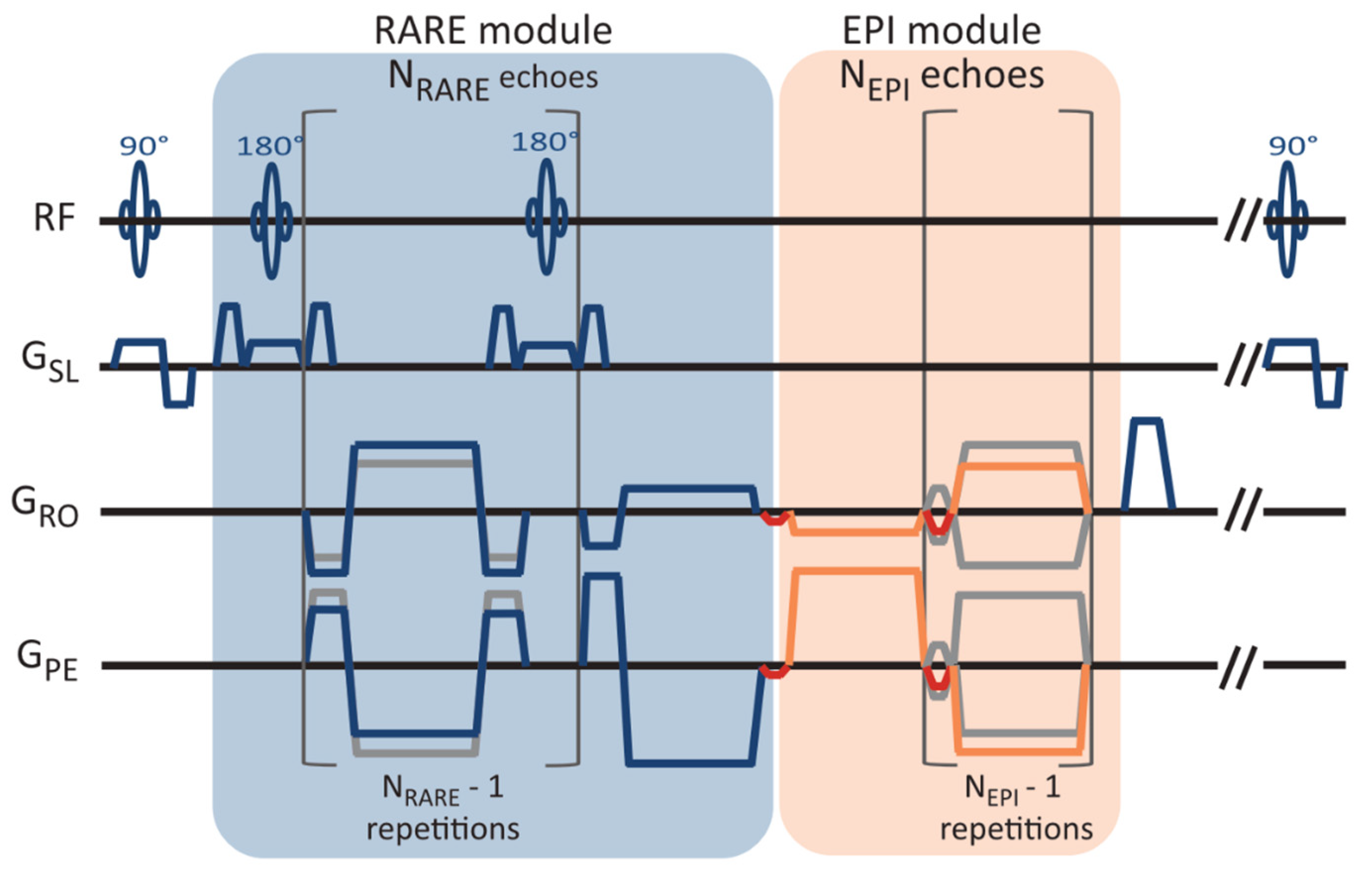
In 2in1-RARE-EPI, the MR signal is first acquired with a RARE module (T
2 decay), followed by the acquisition with an EPI module (T
2* decay). A pulse sequence diagram of 2in1-RARE-EPI is depicted in
Figure 1. In the EPI module, transitions between the k-space spokes are realized by small blip gradients.
The MR data were acquired with 2in1-RARE-EPI at 3.0 T (Siemens Magnetom SkyraFit, Erlangen, Germany, maximum gradient strength, 43 mT/m; maximum slew rate 180.18 mT/m/ms) using the body RF coil for transmission and a 32-channel head RF coil (Siemens, Erlangen, Germany) for signal reception. The radial k-space data were corrected for gradient delays based on a calibration scan acquired prior to each scan (TACalib = 32 s). The following imaging parameters were used: FOV = (232 × 232) mm2, matrix size = 256 × 256, slice thickness = 5 mm, no. of slices = 3, TR = 2000 ms, NRARE = 14, NEPI = 18, echo-spacing (RARE/EPI) = 6.5 ms/2.3 ms, receiver bandwidth = 610 Hz/px, no. of shots (NS) = 200, acquisition time (TA) = TACalib + NS*TR = 07:12 min. For the phantom study, a single slice and FOV = (212 × 212) mm2 were used. The acquisition of 200 shots with a matrix size of 256 × 256 corresponds to an undersampling factor of R = 2 for the TE images.
2.2. Phantom Study
The phantom was designed to mimic the T2 and T2* of brain tissue, and contained 12 plastic tubes (volume = 15 mL, diameter = 15 mm), filled with water-based solutions of the iron oxide nanoparticle-based contrast agent Resovist (Schering, Berlin, Germany). The iron oxide nanoparticles decrease T2 and T2* of the solvent, depending on their concentration in the solution. For the phantom, different solutions with iron concentrations ranging between 2.3 to 12.3 μg Fe/mL were used. Specifically, the tubes were filled with solutions of the following iron concentrations (from left to right and top to bottom): 5.9, 4.6, 6.15, 6.15, 4.01, 4.01, 2.95, 2.95, 2.3, 2.3, 12.3, 8.02 μg Fe/mL and 3.51 μg Fe/mL outside the tubes.
2.3. In Vivo Study
The in vivo feasibility study included three healthy volunteers (1 female/2 male, age = 31–46 years, body mass index (BMI) = 23.6–25.9 kg/m2) and four MS patients (3 female/1 male, age = 30–39 years, BMI = 22.3–34.9 kg/m2). For the in vivo study including healthy volunteers, three slices were acquired, which covered the lateral ventricles. For the in vivo study including MS patients, three slices covering MS specific lesions were acquired, which were selected based on a 2D T2-weighted RARE scan.
2.4. T2 and T2* Mapping
In 2in1-RARE-EPI, the MR signal is first acquired with a RARE module (T
2 decay), followed by the acquisition with an EPI module (T
2* decay). For T
2 and T
2* mapping, a linear least-square fit was applied to the images reconstructed from k-space data acquired at the same echo times (TEs) within the echo train. For T
2 mapping, the first echo was excluded from the fit to limit the effect of stimulated echoes. This approach is generally effective at reducing stimulated echo contamination, however, it may still result in erroneous estimations of T
2, particularly for very low T
2 values [
24].
2.5. Undersampling, Data Pre-Processing, and CS-Reconstruction
The two-fold radially-undersampled 2in1-RARE-EPI data, used as reference, were undersampled at each TE by removing every nth k-space spoke. Undersampling factors of R
extra = 1, 2, 4, 6, 8, 10, and 12 were investigated. This undersampling scheme corresponds to an effective acceleration of R
eff = 2–24. For each receive channel, non-regularized reconstructions of the first TE images were obtained with the Michigan Image Reconstruction Toolbox (MIRT) NUFFT [
25,
26] for the RARE and EPI modules. Based on these images, coil sensitivities were computed with the ESPIRiT method [
27,
28] implemented in the Berkeley Advanced Reconstruction Toolbox (BART, v0.7.00) [
29,
30,
31] for each undersampling factor and module. K-space noise levels and correlations were estimated from background regions in the 1D inverse Fourier transform along the frequency encoding direction. Noise pre-whitening using the Cholesky decomposition of the inverse covariance matrix was performed [
32,
33]. Individual echo parallel imaging CS-reconstructions were computed with wavelet regularization using the Fast Iterative Soft-Thresholding Algorithm implemented in BART [
34,
35,
36,
37]. Automatic optimization of the regularization strength (λ) is essential to ensure reproducibility and reliability of the results [
38]. We employed an adapted version of the discrepancy principle [
39,
40,
41]. Given radial non-uniform Fourier transform
and coil sensitivities
S, the expected quadratic deviation of a true, but unknown, image
rt from the measured data
y is
where
is the number of frequency encoding points,
the number of spokes,
the number of channels, and
the noise standard deviation in the real and imaginary channels. The discrepancy principle consists of finding a value of
λ such that
for CS-reconstruction
. However, implementation of the discrepancy principle, and the CS-reconstruction in general, requires use of a non-uniform fast Fourier transform (
) to limit computation times, and data-derived coil sensitivities
, both of which introduce errors, such that the minimal attainable deviation exceeds the noise level for high SNR data:
The NUFFT and coil sensitivity induced errors are proportional to the signal level, and thus highest in the k-space center, while the measurement noise is uniformly distributed. We exploited this fact by considering only the k-space periphery in the computation of the deviation of the reconstruction from the measured data. For this purpose, we selected only the highest
spatial frequencies on each spoke using masking matrix
. The discrepancy principle condition thus becomes
where
is an additional factor to fine tune the degree of smoothing, which was set to 0.97 in our study [
41]. Importantly, this masking is only applied during the computation of the deviation from the data and not during the CS-reconstruction itself. The Illinois algorithm was employed to find the fitting value of
λ with a tolerance of 0.1% in the data deviation. Using this adapted form of the discrepancy principle, high reconstruction quality could be achieved with automatic tuning for most images. The above condition could not be met for the highest SNR echoes in the RARE module, and for the first echoes of the EPI module without retrospective undersampling. In these cases, a small, fixed
λ value of 2.5 × 10
−5 was employed to ensure the reduction of aliasing artifacts with only minimal deviation from the measured data.
2.6. Assessment of the Effect of Acceleration on T2 and T2* Mapping
To assess the feasibility of undersampling, regression and Bland–Altman plot analyses were performed for every undersampling factor. T
2 and T
2* derived from CS-reconstruction of the undersampled data were benchmarked against T
2 and T
2* obtained from CS-reconstruction of the reference data (R
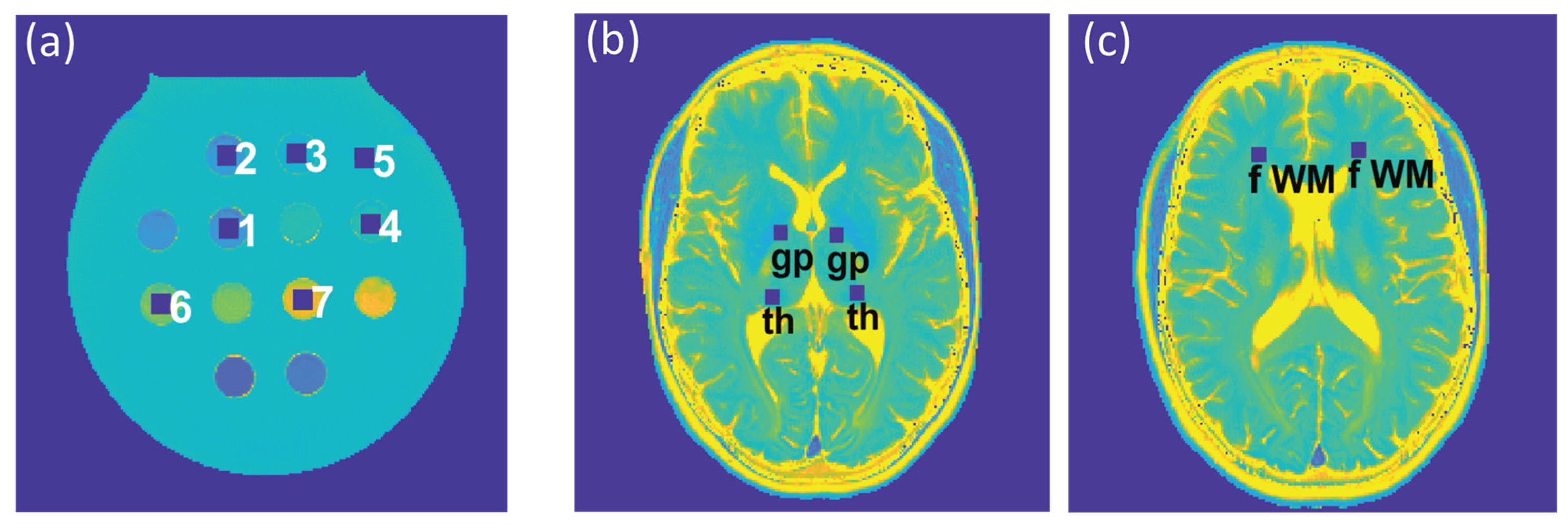
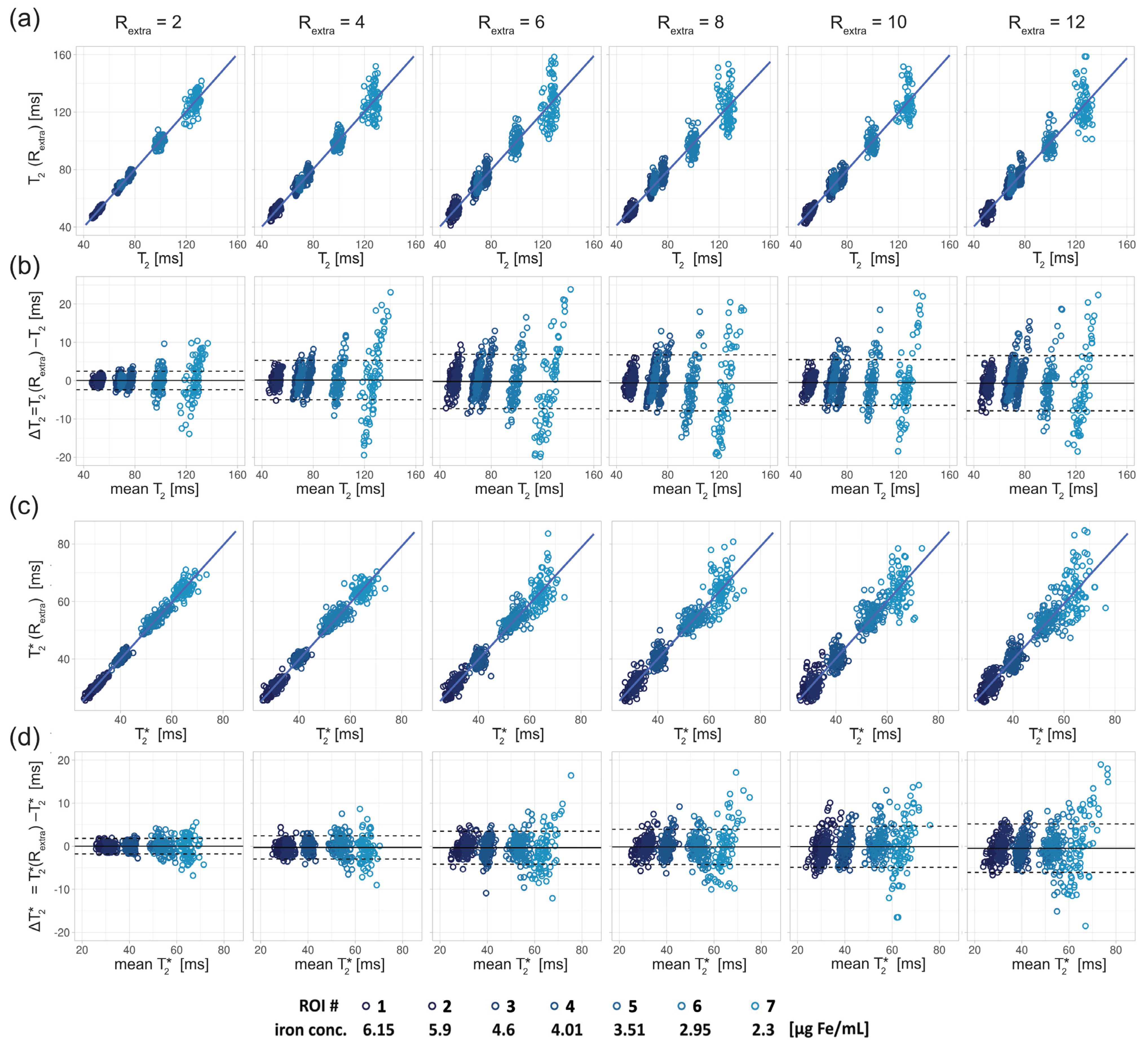
extra = 1). For analysis of the phantom study, seven ROIs (size = 9 × 9 pixels) were placed within the phantom (
Figure 2a), corresponding to the position of the plastic tubes containing the varying iron concentrations. For analysis of the T
2 and T
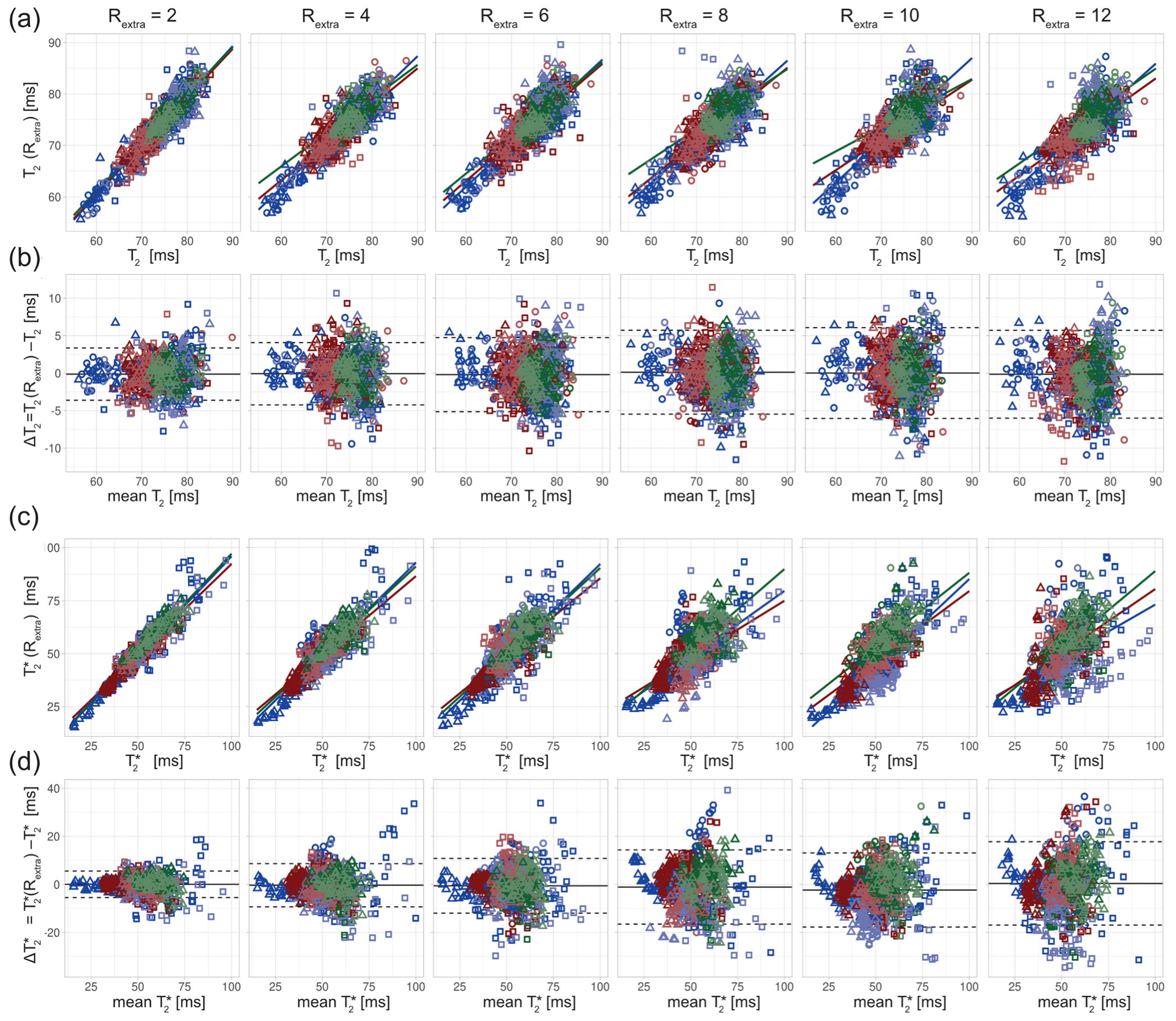
2* maps obtained from healthy volunteers, six ROIs (size = 7 × 7 pixels) were selected for each subject, which were placed within the following anatomical brain regions: the globus pallidus, thalamus, and frontal (periventricular) white matter, in both, the left and right hemisphere (
Figure 2b,c). For analysis of the T
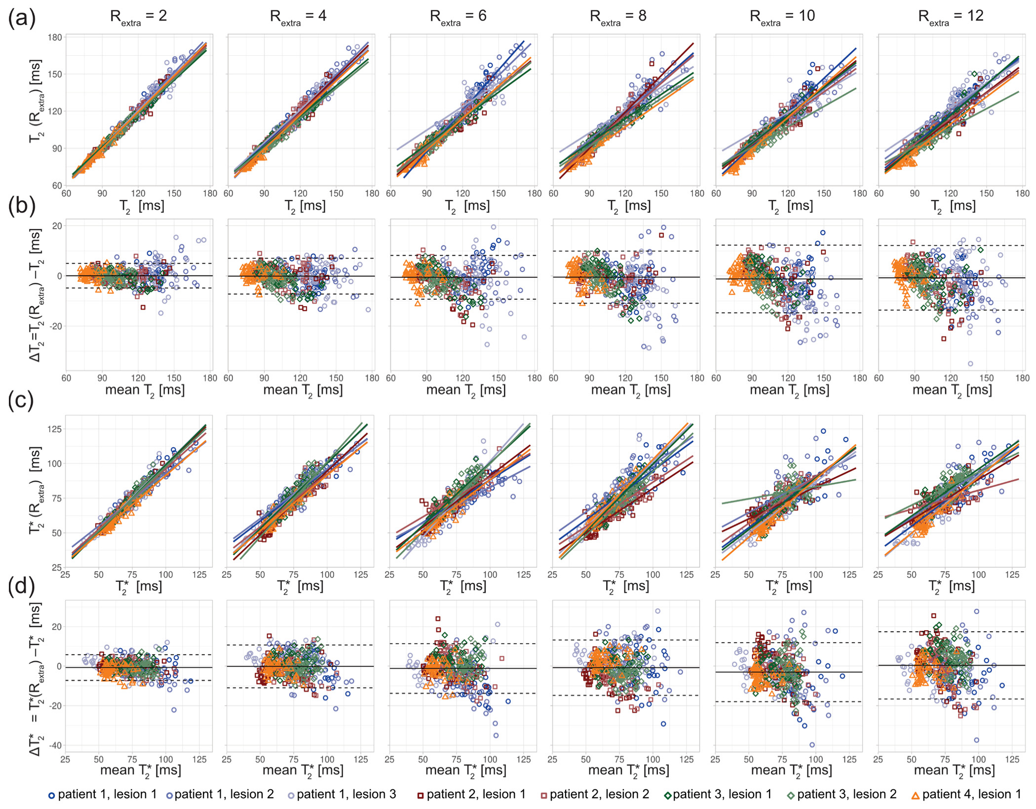
2 and T
2* maps obtained from the patient cohort, eight ROIs (size = 7 × 7 pixels) were selected to cover MS lesions identified in four patients.
Multiple linear regression was used to assess the agreement between the reference and undersampled data, which also takes into account the effects of ROI and subject, and their interaction. For the Bland–Altman plot analyses, the median of the T2 and T2* differences, and and the interquartile range (IQR) were used to calculate the limits-of-agreement (LOAs) according to . since it was observed that the differences of T2 and T2* values among the reference and undersampled data did not follow a Gaussian distribution in all cases.
Furthermore, the median absolute percentage error (MAPE) of T
2 and T
2* derived from undersampled 2in1-RARE-EPI was calculated relative to the corresponding T
2 and T
2* deduced from the CS-reconstruction of the 2in1-RARE-EPI reference (R
extra = 1) according to:
where M denotes the median and T
2(*
)(R
extra) and T
2(*
) the T
2 and T
2* values derived from 2in1-RARE-EPI with and without retrospective undersampling, respectively. The calculation of the MAPE was performed for the same ROIs used for the regression and Bland–Altman plot analyses. Differences in MAPE among R
extra factors were analyzed using the non-parametric repeated-measures Friedman test, followed by the Dunn’s post-hoc test with the Benjamini–Hochberg correction for multiple comparisons. Data were analyzed using R v.3.6.3.
3. Results
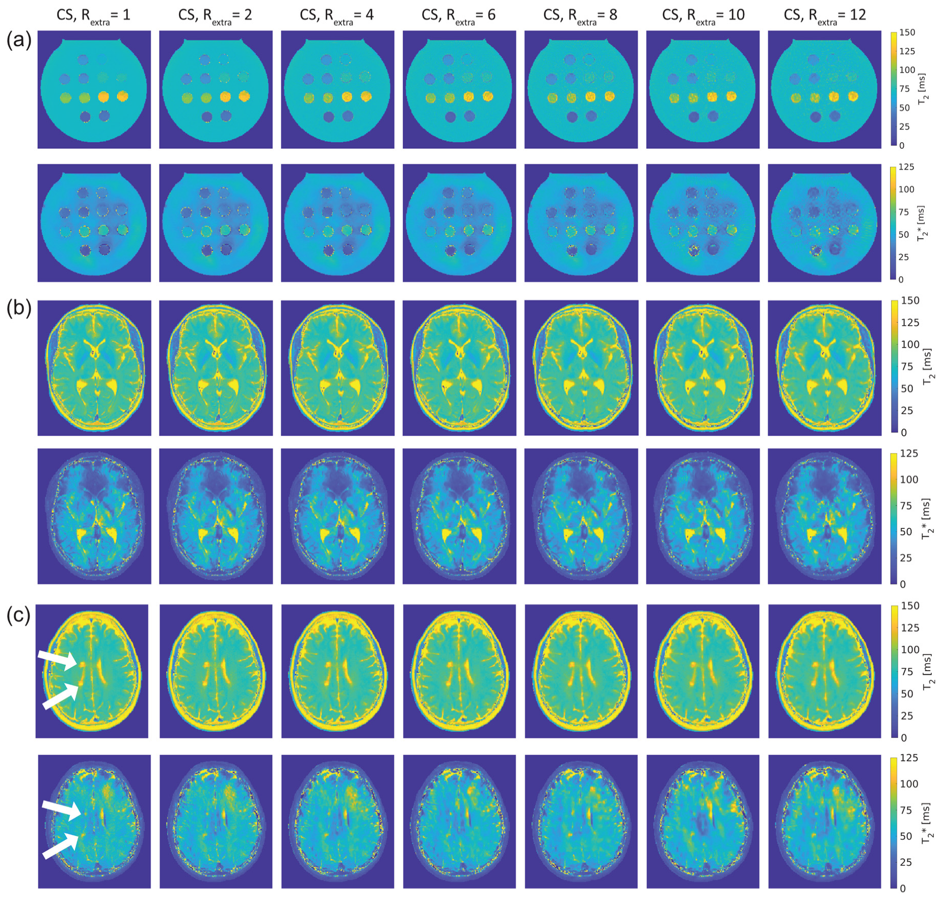
Figure 3 shows T
2 and T
2* maps of the phantom and in vivo studies obtained with 2in1-RARE-EPI for R
extra = 1–12.
Figure 3a shows the T
2 and T
2* maps of the phantom. For the T
2 maps, increasing the undersampling rate to R
extr ≥ 6 (TA reduced to ≤01:39 min) resulted in a minor increase in T
2 for low iron concentrations (T
2(R
extra) ≥ 100 ms). Despite this, no visible change in the T
2 maps was apparent. In the T
2* maps, undersampling artifacts were apparent at R
extra = 8 and became more pronounced with increasing undersampling.
Figure 3b shows T
2 and T
2* maps of the brain of a healthy 30-year-old female volunteer. Increasing undersampling to R
extra = 10 (TA reduced to 01:12 min) resulted in a minor reduction of high spatial frequency information, which became apparent in the small gyri of the brain.
The T
2 and T
2* maps of the brain of a 30-year-old female MS patient are depicted in
Figure 3c. As in the case of the healthy volunteers, increasing undersampling to R
extra = 10 resulted in a minor reduction of high spatial frequency information. The periventricular MS lesions were clearly delineated up to R
extra = 12 in the T
2 maps. In T
2* maps, these lesions were clearly delineated up to R
extra = 10.
For closer examination, the results of the regression and Bland–Altman analyses are depicted in
Figure 4,
Figure 5 and
Figure 6.
For the phantom study, T
2 depicted in the scatter (
Figure 4a) and Bland–Altman plots (
Figure 4b) showed increased variance with increasing undersampling. The multiple linear regression showed a decrease in the adjusted R
2 with increased undersampling for T
2 (0.99, 0.97, 0.92, 0.94, 0.93, 0.92 for R
extra = 2–12, respectively) and T
2* (0.99, 0.99, 0.96, 0.95, 0.94, 0.89 for R
extra = 2–12, respectively). This corresponds to a decrease of the adjusted R
2 of 7% and 10% for the T
2 and T
2*, respectively, when increasing R
extra from 2 to 12. For T
2, a minor increase of the limits-of-agreement (LOAs) from −2.35 ms and 2.46 ms at R
extra = 2 to −7.41 ms and 6.16 ms at R
extra = 12 (TA reduced to 01:06 min) was observed. The median of the T
2 differences showed a minor decrease from 0.05 ms at R
extra = 2 to −0.62 ms at R
extra = 12. These results show that 2in1-RARE-EPI-based T
2 mapping supports high undersampling in conjunction with CS reconstruction. For T
2*, the scatter plots (
Figure 4c) and Bland–Altman plots (
Figure 4d) revealed an increase in the variance. T
2* showed a minor increase of the LOAs from −1.80 ms and 1.81 ms at R
extra = 2 to −6.07 ms and 5.07 ms at R
extra = 12. The median of the T
2* differences decreased from −0.01 ms at R
extra = 2 to −0.50 ms at R
extra = 12. These results demonstrate that 2in1-RARE-EPI-based T
2* mapping supports high undersampling in conjunction with CS reconstruction.
The in vivo study in healthy volunteers showed increased variance of T
2 and T
2* with increasing undersampling (
Figure 5). The multiple linear regression showed a decrease in the adjusted R
2 with increased undersampling for T
2 (0.85, 0.79, 0.72, 0.69, 0.67, 0.70 for R
extra = 2–12, respectively) and T
2* (0.90, 0.79, 0.71, 0.59, 0.71, 0.41 for R
extra = 2–12, respectively). This corresponds to a decrease of the adjusted R
2 of 18% and 54% for the T
2 and T
2*, respectively, when increasing R
extra from 2 to 12. The adjusted R
2 of T
2* at R
extra = 8 is decreased by 34% relative to R
extra = 2. The results of the Bland–Altman plot analysis of T
2 showed a minor increase of the LOAs from −3.62 ms and 3.36 ms at R
extra = 2 to −6.00 ms and 5.71 ms at R
extra = 12. The median of the T
2 differences was −0.13 ms at R
extra = 2 and −0.15 at R
extra = 12. The Bland–Altman plot analysis of T
2* showed an increase of the LOAs from −5.48 ms and 5.55 ms at R
extra = 2 to −16.95 ms and 17.76 ms at R
extra = 12. The median of the T
2* differences increased from −0.04 ms at R
extra = 2 to 0.40 ms at R
extra = 12.
The in vivo study in MS patients revealed an increase in the T
2 variance with increasing undersampling for the ROIs covering the lesions (
Figure 6). The scatter plots show a decrease of the slope of the regression lines with increased undersampling for T
2 and T
2* (
Figure 6a,c). The multiple linear regression showed a decrease in the adjusted R
2 with increased undersampling for T
2 (0.98, 0.97, 0.94, 0.92, 0.91, 0.92 for R
extra = 2–12, respectively) and T
2* (0.94, 0.88, 0.80, 0.81, 0.73, 0.75 for R
extra = 2–12, respectively). This corresponds to a decrease of the adjusted R
2 of 6% and 20% for the T
2 and T
2*, respectively, when increasing R
extra from 2 to 12. The Bland–Altman plot analysis showed an increase of the LOAs from −4.86 ms and 4.94 ms at R
extra = 2 to −13.65 ms and 12.09 ms at R
extra = 12. The median decreased from −0.04 ms at R
extra = 2 to −0.78 ms at R
extra = 12. For T
2*, the LOAs obtained from the Bland–Altman analysis increased from −7.27 ms and 5.76 ms at R
extra = 2 to −16.67 ms and 17.42 ms at R
extra = 12. The median of the T
2* differences increased from −0.75 ms at R
extra = 2 to 0.37 ms at R
extra = 12.
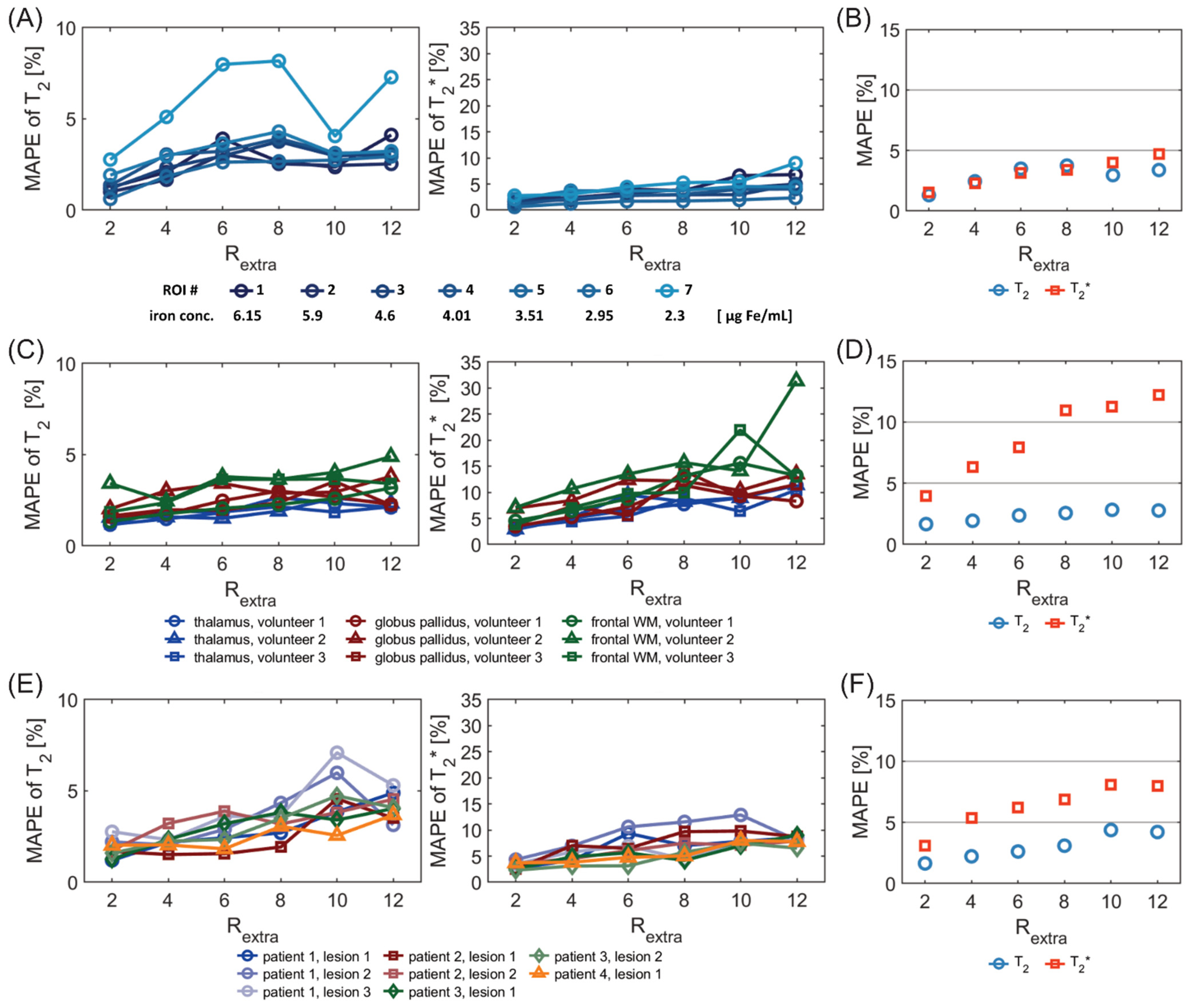
Figure 7A shows the MAPE analysis of T
2 and T
2* for the phantom study. There was a significant difference in the MAPE of T
2 of the 7 ROIs placed within the phantom among different undersampling factors R
extra (
p = 3.8 × 10
−5, Friedman test). There were significant differences of the MAPE of T
2 between R
extra = 6, 8, and 12 and R
extra = 2 (
p = 4.7 × 10
−3, 3.2 × 10
−3, 2.1 × 10
−3, respectively, Dunn’s post-hoc test). The overall MAPE of T
2 (
Figure 7B) for R
extra = 8 was only 3.7%. For T
2*, there were significant differences in the MAPE among the various undersampling factors (
p = 3.1 × 10
−6). There were significant differences between R
extra = 10–12 and R
extra = 2 (2.3 × 10
−2, 4.6 × 10
−4, respectively). The overall MAPE of T
2* (
Figure 7B) for R
extra = 12 was 4.7%.
Figure 7C shows the MAPE of T
2 and T
2* for the in vivo study with healthy volunteers. For the MAPE of T
2, significant differences were obtained among different undersampling factors R
extra (
p = 1.0 × 10
−4) for the six ROIs placed in the brain. There were significant differences of the MAPE of T
2 between R
extra = 8–12 and R
extra = 2 (
p = 7.5 × 10
−3, 5.3 × 10
−3, 7.2 × 10
−3, respectively). This shows the consistency of the T
2 measurement within subjects for R
extra below 8. For T
2*, there were significant differences in the MAPE among the various undersampling factors (
p = 7.3 × 10
−7). There were significant differences of the MAPE of T
2* between R
extra = 6–12 and R
extra = 2 (
p = 1.0 × 10
−2, 2.4 × 10
−4, 3.1 × 10
−4, 3.2 × 10
−5). This shows the consistency of the T
2* measurement within subjects for R
extra below 6. The overall MAPE of T
2 and T
2*(
Figure 7D) for R
extra = 6 was as small as 2.4% and 7.9%, respectively.
Figure 7E shows the MAPE of T
2 and T
2* for the in vivo study with MS patients. There was a significant difference of the MAPE of T
2 values of the eight ROIs, covering MS lesions, among different undersampling factors R
extra (
p = 1.5 × 10
−5). There were significant differences of the MAPE of T
2 between R
extra = 8–12 and R
extra = 2 (
p= 1.0 × 10
−2, 1.7 × 10
−4, 1.0 × 10
−4, respectively). This shows the consistency of the T
2 measurement within subjects for R
extra below 8. For T
2*, there were significant differences in the MAPE among the various undersampling factors (
p = 1.8 × 10
−4). There were significant differences of the MAPE of T
2* between R
extra = 6–12 and R
extra =2 (
p = 9.4 × 10
−3, 6.7 × 10
−3, 7.4 × 10
−5, 7.7 × 10
−5, respectively
,). This shows the consistency of the T
2* measurement within subjects for R
extra below 6. The overall MAPE of T
2 and T
2* (
Figure 7F) for R
extra = 6 was 2.6% and 6.2%, respectively.
4. Discussion
In this study, we demonstrated the feasibility of highly accelerated simultaneous T2 and T2* mapping using a radially-undersampled RARE-EPI hybrid in conjunction with CS-reconstruction. The findings from this feasibility study support the application of quantitative T2 and T2* mapping of the brain in clinical practice, which could be utilized for broader clinical studies on the potential of T2 and T2* as imaging biomarkers in MS.
The regression and Bland–Altman analysis revealed an increase of the variance of the T2 and T2* values with increasing undersampling for both the phantom experiments and the in vivo studies. The Bland–Altman analysis showed that the median of the differences of T2 and T2* values were close to zero in all cases, for all investigated undersampling factors, which suggests that an increase in undersampling does not introduce a systematic bias in T2 and T2*.
The higher variance in ROIs 6 and 7 can be attributed to the fact that there is a large and sharp signal drop at the edge of the plastic tubes for these ROIs due to the difference in T2 values of the solution within the tube and that in the surrounding body of the phantom. This leads to increased variance of T2 values caused by more pronounced Gibbs ringing artifacts. Furthermore, residual aliasing artifacts which are not fully compensated by the CS reconstruction might have a higher impact on ROIs 6 and 7, as the mislocated signal stemming from the phantom body deviates more in T2/T2* than for the other ROIs.
In addition, the higher variance in ROI 6 can be attributed to the higher T2 and T2* values within the ROI, i.e., the relative variance of the T2 and T2* values corresponding to ROI 6 does not substantially differ from the relative variances in ROIs 1–5. For ROI 7, the relative variance is increased compared to the other ROIs, which emphasizes the stronger influence of Gibbs ringing and aliasing artifacts in this ROI.
The Bland–Altman plots of the T2 values of MS lesions showed that the T2 differences follow a negative trend, with increasing mean T2 values for higher undersampling factors (Rextra = 8–12). This can likely be explained by the reduction of high spatial frequency information in highly undersampled images, leading to smoothing of the lesion sharpness, and reduced contrast between the lesions and surrounding tissue with lower T2.
The smaller relative decrease of the adjusted R
2 of T
2 and T
2* with increased undersampling in the phantom study compared to the in vivo studies can be explained by the higher degree of sparsity in the phantom images compared to images of the brain, which promotes accurate recovery of true signal intensities for higher undersampling factors [
42]. We observed that the relative decrease of the adjusted R
2 of T
2 and T
2* was lower for the in vivo study with MS patients compared to the healthy volunteers. This can be attributed to the fact that in the case of MS patients, the T
2 and T
2* values within all ROIs have a larger range than in the ROIs of the healthy volunteers, and thus the additional variance contributed by the undersampling is proportionally smaller.
A previous study that investigated the performance of R
2* mapping based on 3D single point imaging (SPI) with CS reconstruction in ex vivo rat tissue and an in vitro cell phantom [
15] shows a relative decrease of the R
2 of about 10–12% for an increase of the undersampling factor from 2 to 10, which is lower than the values observed in our in vivo studies. However, there a number of differences between the two studies that can explain these discrepancies. In the SPI approach, only one k-space point is sampled within a TR, which increases the accuracy of R
2* measurements, due to a higher sampling rate of the signal decay, but at the expanse of considerably longer scan times. Furthermore, the 3D single point sampling of k-space allows for a higher degree of freedom in the undersampling pattern, which can substantially increase the performance of CS reconstruction at high undersampling factors [
36,
43]. This motivates the future investigation of 2in1-RARE-EPI using 3D k-space sampling schemes.
The analysis showed that the MAPE of T2* is higher and increases more strongly with increasing undersampling compared to the MAPE of T2. This can be explained by the hybrid acquisition of the MR signal in 2in1-RARE-EPI, in which the MR signal is first acquired with a RARE module to capture the T2 decay, followed by the acquisition with an EPI echo-train to capture the T2* decay. This results in a lower SNR of the TE images used for T2* mapping, which manifests as an increased MAPE of T2*. Notwithstanding this SNR constraint, the overall MAPE of T2* was <5% in the phantom studies for Rextra ≤ 12, and <8% in the in vivo studies for Rextra ≤ 6. The overall MAPE of T2 remained <4.4% for Rextra ≤ 12 in the phantom and in vivo studies.
Due to the consecutive sampling of the T2 and T2* decay within each TR, the measurement of T2* values could be impaired for tissues exhibiting very low T2 values. This could be due, e.g., as a result of increased iron deposition, which is a pathological feature of some neurodegenerative diseases, including MS. The lowest T2 values of the tissues investigated in the current study are about 60 ms, which does not impact the T2* measurement. Evaluating simultaneous T2 and T2* mapping with 2in1-RARE-EPI for lower T2 values will require further studies, including an adaptation of the length of the RARE and EPI module to achieve optimal results.
In this study, we used a limited slice coverage (n = 3, slice thickness = 5 mm) to demonstrate the feasibility of our approach. This could be easily scaled up to meet the needs of clinical applications, by reducing the slice thickness and increasing the total number of slices acquired. Reduced slice thickness would also mitigate partial volume effects and result in a better coverage of lesions. Given the high SNR we observed for the 2in1-RARE-EPI using the imaging parameters of the current study, we expect the results presented here to also hold for lower slice thicknesses. The long TR used in the 2in1-RARE-EPI will allow for acquisition of additional slices without increasing the acquisition time.
The scan time reduction shown in this work will benefit patient compliance, and enhances the robustness to bulk motion. With an extra undersampling factor of R
extra = 6 (R
eff = 12), the acquisition time for simultaneous T
2 and T
2* mapping can be reduced from 07:12 min to 01:39 min. An extra undersampling of R
extra = 12 (R
eff = 24) permits a scan time as short as 01:06 min. The 2in1-RARE-EPI approach is compatible with the concept of using different undersampling rates for the RARE module and for the EPI module. This approach would permit an improvement of the RF deposition economy of the RARE module. Even further scan time reductions could be achieved by employing simultaneous multi-slice imaging techniques which are compatible with 2in1-RARE-EPI [
6,
44,
45,
46].
The current study is a proof-of-concept demonstration of the feasibility of using undersampled 2in1-RARE-EPI in a realistic clinical context, and was not designed or powered to detect group differences. Further clinical studies with larger numbers of patients will be needed to robustly test the sensitivity to group differences.


 ,
, 
